Non-linear charge and energy dynamics of an adiabatically driven interacting quantum dot

We consider the system of Fig. 1. A driven quantum dot is connected to a normal lead of free electrons at zero temperature and chemical potential $\mu$. The full setup is described by an Anderson Hamiltonian,

The first term describes the dot

with $n_{d\sigma}$ denoting the number operator with spin $\sigma=\uparrow,\downarrow$, $U$ is the Coulomb repulsion, and $\varepsilon_{d,\sigma}(t)=\varepsilon_{0}+s_{\sigma}\frac{\delta_{Z}}{2}+{\cal V}_{g}(t)$ is the single-particle energy modulated by the applied gate voltage $V_{g}(t)$, with ${\cal V}_{g}(t)=eV_{g}(t)=V_{0}\sin(\Omega t)$, $\delta_{Z}$ is the Zeeman splitting due to the presence of an external magnetic field, $s_{\sigma}=\pm 1$ for $\sigma=\uparrow,\downarrow$, and $-e$ is the charge of the electron. The reservoir is described by the Hamiltonian $H_{\text{res}}=\sum_{\sigma,k}\epsilon_{k}c_{k\sigma}^{\dagger}c_{k\sigma}$, which is assumed to have a constant density of states within a bandwidth $2D$. The coupling between dot and reservoir is $H_{T}=V_{c}\sum_{k\sigma}\left[c_{k\sigma}^{\dagger}d_{\sigma}+h.c\right]$.

The conservation of the charge in the full system implies

where $n_{d\sigma}(t)\equiv\langle n_{d\sigma}(t)\rangle$ is the occupancy of the dot by electrons with spin $\sigma$ at time $t$, $I_{C,\sigma}(t)$ is the contribution of the electrons with spin $\sigma$ to the charge current flowing out of the dot at time $t$, and $e>0$ the elementary charge.

The power developed by the external ac source on the electron system is defined as [20] $P_{\rm ac}(t)=-\langle\partial H/\partial t\rangle=-e\sum_{\sigma}n_{d\sigma}(t)\dot{V}_{g}(t)$. This leads to a net heat production in the electron system at a rate $\dot{Q}(t)=-P_{\rm ac}(t)$. [21] We find it convenient to define the power

such that $P>0$ implies work delivered from the electron system against the ac sources. With this definition, the rate for the heat production in the electron system reads $\dot{Q}(t)=P(t)=P_{\mathrm{cons}}(t)+P_{\mathrm{diss}}(t)$. [22] This power contains a purely ac component $P_{\mathrm{cons}}(t)$ associated to the reversible heat produced by the conservative (Born-Oppenheimer) forces, and a dissipative component $P_{\mathrm{diss}}(t)$ with a non-zero time average.

The dynamics of the heat production and the charge current is fully determined by $n_{d\sigma}(t)$. For low frequencies, the latter can be calculated within the adiabatic formalism of Ref.  24, which corresponds to linear-response in $\dot{V}_{g}(t)$ (see Appendix A). The result is

where $n_{f,\sigma}(t)\equiv\langle n_{d\sigma}\rangle_{t}$ is the snapshot occupancy of the dot, evaluated with the exact equilibrium density matrix $\rho_{t}$ corresponding to the Hamiltonian $H(t)$ frozen at the time $t$. The coefficient of the second term is

with $\overline{\uparrow}=\downarrow$ and $\overline{\downarrow}=\uparrow$. $\chi_{t}^{\sigma\sigma^{\prime}}(\omega)$ is the Fourier transform of the charge susceptibility $\chi_{t}^{\sigma\sigma^{\prime}}(t-t^{\prime})=-i\theta(t-t^{\prime})\langle[n_{d\sigma}(t),n_{d\sigma^{\prime}}(t^{\prime})]\rangle_{t}$ evaluated with $\rho_{t}$.

In the case of the system with applied magnetic field, it is appropriate to analyze separately the current and the power developed by electrons with the different spin components. The current per spin can be calculated by the derivative of Eq. (6)

where the first term is related to the static charge susceptibility through $dn_{f,\sigma}/dV_{g}=\chi_{t}^{\sigma\sigma}(0)$.

The frozen component $n_{f,\sigma}(t)$ contributes to the conservative component of this power, while the last term of Eq.  (6) contributes to the non-conservative one. They read, respectively

It is important to notice that the non-conservative components $P_{\rm\sigma}(t)$ are not necessarily fully dissipative. They certainly contribute to the total dissipation, but they may also contain a non-dissipative ”exchange” part $P_{\rm ex}(t)$, such that $P_{\uparrow(\downarrow)}(t)=\pm P_{\rm ex}(t)+P_{\rm diss,\uparrow(\downarrow)}(t)$. The exchange component is associated to time-dependent induced forces that are proportional to $\dot{V}_{g}(t)$. In this sense, these forces are akin to the ”Lorentz” forces discussed in Ref. 25. However, in the present case they may develop work only instantaneously while the average over one period is zero.

The total power has conservative $P_{\rm cons}(t)=\sum_{\sigma}P_{\mathrm{cons},\sigma}(t)$, and dissipative components $P_{\rm diss}(t)=\sum_{\sigma}P_{\mathrm{diss},\sigma}(t)$, which read

For later use we also define

When performing the averages over one period $\tau=2\pi/\Omega$ for these two contributions to the power, $\overline{P}_{\mathrm{cons,diss}}=(1/\tau)\int_{0}^{\tau}dtP_{\mathrm{cons,diss}}(t)$, we find $\overline{P}_{\mathrm{cons}}=0$ and $\overline{P}_{\mathrm{diss}}\geq 0$ in accordance to the second law of thermodynamics.

We see that the full charge and energy dynamics in the adiabatic regime is completely determined by the behavior of the frozen charge susceptibility $\chi_{t}^{\sigma\sigma^{\prime}}(\omega)$, irrespective of the strength of the interactions and the amplitude of the driving potential.

We now discuss the representation of the equations for the dynamics of the charge and energy introduced in the previous section, in terms of a classical non-linear circuit. We find it convenient to treat the two spin channels separately as a circuit with two branches (one for each spin species) connected in parallel to the ac source, as sketched in Fig. 2. Each branch contains a capacitance $C_{\sigma}(t)$ in series with a resistance $R_{\sigma}(t)$.

We assume that the equation relating the current through each branch of the circuit with the potential $V_{g}(t)$ is

As discussed in Appendix B, this equation corresponds to a true macroscopic classical RC circuit in the non-linear low-frequency regime satisfying $\Omega R_{\sigma}I_{\sigma}\ll 1$. Identifying linear and quadratic terms in $\dot{V_{g}}$ in the above equation with those of the quantum current Eq. (8) one obtains

Here, unlike the linear case, the non-linear capacitance $C_{\sigma}(t)$ and resistance $R_{\sigma}(t)$ are, in general, functions of $t$. In terms of these coefficients, the dissipated power (10) reads

We see that for the case where $R_{\sigma}(t)=R_{0}$, Eq. (14) reduces to the IJL described by Eq. (1), which is immediately derived by retaining only the first term of Eq. (8). In fact, the latter is the only term of Eq. (8) which has a contribution $\propto[\dot{V}_{g}(t)]^{2}$ to $P_{\mathrm{diss}}(t)$, since $d\Lambda_{\sigma}(t)/dt=\left(d\Lambda_{\sigma}(t)/dV_{g}(t)\right)\dot{V_{g}}(t)$.

The above equations are exact and valid in general within the adiabatic regime. However, in order to establish a meaningful correspondence between the charge and energy dynamics of the quantum system and the classical circuit of Fig. 2, the coefficients defined in Eq. (13) should also verify $R_{\sigma}(t)>0$ and $C_{\sigma}(t)>0$. As we will discuss in detail in the next sections, such a correspondence is valid in the system without spin polarization ($\delta_{Z}=0$) for arbitrary Coulomb interaction $U$, as well as in the non-interacting case ($U=0$) with arbitrary $\delta_{Z}$. We also argue in Sections IV and V that the dynamics of the driven interacting quantum dot in the presence of a magnetic field cannot be interpreted in terms of the circuit of Fig. 2.

The expressions of the previous sections are completely general and valid for arbitrary temperatures, for non-interacting as well as interacting systems. We now relate them to the non-interacting results for spinless electrons of Refs.   12, 19, 21, 24. This corresponds to the Hamiltonian (3) with $U=\delta_{Z}=0$ and with only one spin species. Following Refs.  27, 19, 21, we get

where $\rho_{f}(t,\epsilon)=(\Delta/\pi)/\left[\left(\epsilon-\varepsilon_{d}(t)\right)^{2}+\Delta^{2}\right]$ is the non-interacting frozen density of states of the quantum dot connected to a reservoir with constant density of states $\nu$, $\Delta=\pi\nu V_{c}^{2}$, and $f(\epsilon)$ is the Fermi distribution function.

The resistance can be directly calculated from Eq. (13). At $T=0$, we have $-\partial f/\partial\epsilon=\delta(\epsilon-\mu)$. Hence, the coefficients simplify to $C(t)=e^{2}\rho_{f}(t,\mu)$ and $R(t)=R_{0}=h/(2e^{2})$. The latter corresponds to the universal resistance quantum for a single channel. By substituting these expressions in $P_{\mathrm{diss}}(t)$ and $I_{C}(t)$, and keeping terms up to $\mathcal{O}(\dot{V}_{g}^{2})$, we recover the IJL of Eq. (1) as in Ref. 19. Interestingly, we get the same expression of the current $I_{C}(t)$ in the non-interacting limit as the one of Ref.  12. However the definition of $R(t)$ presented there differs from the definition of Eq. (13) with $\Lambda(t)$ given by Eq. (15). Such difference should be traced back to the equation for the non-linear circuit (12). Unlike the one considered in Ref.  12, Eq. (12) includes the factor $RC$ inside the time-derivative of the second term. The structure of the latter Eq. is motivated by the adiabatic expansion of the occupancy Eq. (6), by identifying the coefficient $\Lambda(t)$ as the dissipative contribution. Remarkably, our definition of $R(t)$ can be easily related to $R_{0}$ in the limit of $T=0$ and it consistently leads to the Joule law of Eq.  (1), while it is also in agreement with the effective resistance defining the noise. [12]

We now consider the case with $U=0$ and arbitrary $\delta_{Z}$. Notice that for non-interacting electrons the ”crossed-susceptibility” $\chi_{t}^{\sigma,\overline{\sigma}}(\omega)=0$. Hence the coefficient $\Lambda_{\sigma}(t)$ is fully determined by the susceptibilities $\chi_{t}^{\sigma,\sigma}(\omega)$. The calculations of Refs. 12, 19, 21, 24 can be easily extended to non-interacting electrons with spin.

The frozen occupancy of the quantum dot with spin $\sigma$ is

where $\rho_{f,\sigma}(t,\epsilon)=(\Delta_{\sigma}/\pi)/\left[\left(\epsilon-\varepsilon_{d,\sigma}(t)\right)^{2}+\Delta_{\sigma}^{2}\right]$. For this model $\partial\rho_{f,\sigma}(t,\epsilon)/\partial t=e\left(\partial\rho_{f,\sigma}(t,\epsilon)/\partial\epsilon\right)\dot{V}_{g}(t)$. Hence, after integrating by parts the above equation, we get for $T=0$

In addition, we get an expression like (15) for each spin orientation $\sigma$. For $T=0$, it reads

which is a special case of the Korringa-Shiba (KS) law discussed in the next section. Inserting these expressions in Eqs. (13) we obtain $R_{\sigma}(t)=R_{0}$. Substituting in (10), we see that the dissipated power is ruled by the IJL of Eq. (1).

Therefore, for non-interacting electrons, Korringa-Shiba law of Eq. (18) implies that there is a full one-to one correspondence between the charge and energy dynamics of the driven electron system and the two-branch circuit sketched in Fig. 2, with resistances $R_{\sigma}(t)=R_{0}$, even when the electrons are spin-polarized. This also means that the ac forces associated to the induced charge for each spin orientation dissipate heat in the form of a Joule law, $P_{\sigma}(t)=R_{0}[I_{C,\sigma}(t)]^{2}=P_{\rm Joule,\sigma}(t)$. Hence, $P_{\rm diss}(t)=\sum_{\sigma}P_{\rm Joule,\sigma}(t)=R_{q}[I_{C}(t)]^{2}$, with $I_{C}(t)=\sum_{\sigma}I_{C,\sigma}(t)$ and $R_{q}=R_{0}/2$.

For interacting electrons, the crossed susceptibility $\chi_{t}^{\sigma,\overline{\sigma}}(\omega)$ contributes to the coefficient $\Lambda_{\sigma}(t)$, in addition to $\chi_{t}^{\sigma,\sigma}(\omega)$. For Fermi liquids, an important relation exists for the total charge susceptibility $\chi_{t}^{c}(\omega)=\sum_{\sigma,\sigma^{\prime}}\chi_{t}^{\sigma,\sigma^{\prime}}(\omega)$, which receives the name of Korringa-Shiba law. [26] In the non-interacting case, it is expressed in Eq. (18). In the interacting case, it is a non-trivial result, which was originally proved by Shiba in the Anderson model [26] and later generalized by Fillipone et al. when a magnetic field is also considered. [10, 11] It reads

This relation has been used to study the present problem within the linear response regime. [7, 8, 9, 10, 11] Here, we show that the Korringa-Shiba law Eq. (19) is equivalent to the instantaneous Joule law Eq. (1), even in the presence of a magnetic field and also in the non-linear response regime.

In fact, from Eqs. (7) and (10) and taking into account that Eq. (19) is satisfied, we have

On the other hand, the -up to ${\cal O}(\dot{V}_{g}(t))$- charge current with spin $\sigma$ is given by the first term of Eq. (8) and reads

Then, substituting in Eq. (20), we get

which is, precisely, the IJL. This result holds for electrons with and without spin polarization, in the non-linear as well as in the linear regimes.

In the case of non-polarized electrons, where the two spin orientations are equivalent. The total charge current $I_{C}(t)=\sum_{\sigma}I_{C,\sigma}(t)$ associated to the change in the dot occupancy by up and down spins is given by [see Eqs. (8) and (13)]

with $C(t)=\sum_{\sigma}C_{\sigma}(t)$, and $\Lambda^{c}(t)=\sum_{\sigma}\Lambda_{\sigma}(t)$.

The definition of the resistance given in Eq. (13), along with $C(t)=-e^{2}\chi_{t}^{c}(0)$ and the KS relation Eq. (19), lead to the resistance $R_{0}$ for each spin channel or an equivalent resistance $R_{q}=R_{0}/2$ for the equivalent circuit of Fig.1. In fact, because of the equivalence of both branches of the circuit of Fig. 2, the voltage drop at the middle point between the resistance and capacitance for each branch are the same. Therefore, one can connect this two points with a cable carrying no current and the circuit becomes equivalent to that at the top of Fig. 1, with an effective resistance $R_{q}^{-1}=2R_{0}^{-1}$ in series with the effective capacitance $C(t)=2C_{\sigma}(t)$. In addition, the arguments of the next section as well as the numerical results will show that $C(t)\geq 0$. Hence, for non-polarized electrons, the behavior of the charge and energy dynamics is consistent with the representation of the setup in terms of the parallel circuit of Fig. 2 or the equivalent one of Fig. 1. The charge dynamics is described by Eq. (23) with $e^{2}\Lambda^{c}(t)=R_{q}[C(t)]^{2}$. while the dissipated power obeys the IJL Eq. (22).

In the case of polarized electrons, the two spin orientations are not equivalent and it is not easy to analyze the dynamics by simple analogy to the classical circuit. It is important to notice that the Coulomb interaction effectively renormalizes the gate voltage at a given time. At the mean field level, this can be accounted by an occupancy-dependent term $U\langle n_{f,\overline{\sigma}}\rangle$ which adds to ${\cal V}_{g}(t)$ in the effective local energy experienced by an electron with spin $\sigma$ at the quantum dot. Here, we will analyze the consequence of this effect on the basis of the behavior of the charge susceptibility in the ”random phase approximation” (RPA). In the next section we will present a more accurate analysis based on NRG results.

RPA corresponds to calculating the dynamic susceptibility from the summation of an infinite perturbative series of ”bubble” diagrams. The result in the present case is

where $\chi_{t}^{0\sigma}(\omega)$ is the susceptibility for $U=0$. The latter is a function of the gate voltage $V_{g}(t)$ and satisfies the KS relation (18). The static limit is given by Eq. (17), $\chi_{t}^{0\sigma}(0)=-\rho_{f,\sigma}(\mu)$. In the case of non-polarized electrons, where the two spin orientations are equivalent, we have $\chi_{t}^{\sigma\sigma}(\omega)=\chi_{t}^{0\sigma}(\omega)/\left[1+U\chi_{t}^{0\sigma}(\omega)\right]$. Hence, the calculation of the capacitance gives $C_{\sigma}(t)=C_{\sigma,0}(t)/\left[1+UC_{\sigma,0}(t)/e\right]$, where $C_{\sigma,0}(t)$ is the capacitance of the non-interacting system (17), which indicates that $C_{\sigma}(t)\geq 0$.

In the case of polarized electrons we have situations where $|\chi_{t}^{0\sigma}(0)|\ll|\chi_{t}^{0\overline{\sigma}}(0)|$ or vice versa, in which case Eq. (24) leads to negative values of the coefficient $C_{\sigma}(t)$ for large enough $U$. This corresponds to a current between the reservoir and the dot which opposes to the sense of circulation imposed by the voltage drop. Furthermore, after some algebra from (24) and the KS relation for the non-interacting susceptibilities (18), we can see that in such situations the signs of $\Lambda_{\sigma}(t)$ and $\Lambda_{\overline{\sigma}}(t)$ are opposite. This would correspond to instantaneous exchange of power between the two spin species, $P_{\sigma}(t)\sim P_{\rm ex}(t)\sim-P_{\overline{\sigma}}(t)$. We can interpret this behavior as electrons with spin $\sigma$ receiving energy from the electrons with spin $\overline{\sigma}$ to move against the external voltage drop. In addition to this component, there is a dissipative component of the power satisfying the IJL [see Eq. (22)]. Since the behavior explained above is not expected in a capacitive circuit element, we conclude that the representation of the dynamics of the driven interacting quantum dot in the presence of a magnetic field is not properly represented by a circuit like that of Fig. 2. In the next section, we will verify that such a behavior indeed takes place when the susceptibilities are exactly calculated with NRG.

In a system without spin polarization, the two spin orientations are equivalent and the dynamics of the quantum system is fully equivalent to that of the circuit of Fig. 2 or that with the equivalent components sketched in Fig.1. As argued in the previous section, the two resistances can be simply substituted by the resistance $R_{q}=R_{0}/2$ in series with the capacitance $C(t)=2C_{\uparrow}(t)=2C_{\downarrow}(t)$. The total current circulating through the single branch of the equivalent circuit is given by Eq. (23). The total dissipated power is given by Eq. (10) with $\Lambda^{c}(t)=\sum_{\sigma}\Lambda_{\sigma}(t)$.

The behavior of the time-dependent occupancies for $\uparrow$ and $\downarrow$ spins in the presence of a Zeeman splitting $\delta_{Z}$ at the quantum dot are shown in Fig. 7 for different values of $U$. The upper, middle and bottom panels correspond, respectively to the same parameters as the plot in dot-dashed, dashed and solid lines of Fig. 5, with the additional ingredient of a magnetic field. In all the cases, the dot is in the half-filled configuration at $t=0$ ($n_{f}(0)=1$) and is predominantly occupied by electrons with spins parallel to the direction of the magnetic field (in this case $\downarrow$). The magnitude of the Zeeman splitting is chosen larger than the Kondo temperature $T_{K}$ for all times. Hence, for one electron in the dot, the system is in the local moment regime of the Anderson model with a significant spin polarization.

Starting from the symmetric configuration at $t=0$, the energy of the localized electrons for both spin orientations $\varepsilon_{d,\sigma}(t)$ increases in time and the occupancy of the quantum dot evolves to the empty configuration when $\varepsilon_{d,\downarrow}(t)\sim U/2$ (this situation is however not reached for the largest $U$ considered). As this happens, of course also the local spin of the quantum dot vanishes. After passing through its maximum at $\Omega t=\pi/2$, $\varepsilon_{d,\sigma}(t)$ decreases and the quantum dot becomes again filled with a $\downarrow$ electron when $\varepsilon_{d,\downarrow}(t)\sim U/2$. As $\varepsilon_{d,\sigma}(t)$ continues to decrease towards its minimum at $\Omega t=3\pi/2$, and additional electron occupies the quantum dot when $\varepsilon_{d,\downarrow}(t)\sim-U/2$. This implies again a vanishing total spin at the quantum dot and as a consequence, the magnetic field does not lead to a spin polarization. In fact, we see in all the panels of the figure that the two occupancies differ only for values of the gate voltage where the total mean occupancy is close to one electron, in which case, there is a finite spin polarization at the quantum dot, $\sum_{\sigma}n_{f,\sigma}(t)\neq 0,2$.

We note that for $\varepsilon_{0}=\mu=0$ and any magnetic field the Hamiltonian is invariant under the following transformation: $t\rightarrow-t$ and

assuming a symmetric conduction band such that for any eigenstate $k$ of the isolated band, there is another one $k^{\prime}$ with $\epsilon_{k^{\prime}}=-\epsilon_{k}$. As a consequence of this symmetry, $n_{f,\uparrow}(t)=1-n_{f,\downarrow}(-t)$ as can be seen in the figure.

Focusing on the interval $0<\Omega t<\pi/2$ of Fig. 7, for which the one-site energy of the dot increases, we see that the expected decrease in the occupancy for the majority down spin is accompanied by an increase in the occupancy of the minority up spin, denoting a charge susceptibility of opposite sign for spin up. As already mentioned in Section IV. C, within a mean field description, the effective local energy for spin up is $\varepsilon_{d,\uparrow}(t)=\varepsilon_{0}+\frac{\delta_{Z}}{2}+\mathcal{V}_{g}(t)+Un_{f\downarrow}$, and the increase in $\mathcal{V}_{g}(t)$ is overcome by the decrease in $Un_{f\downarrow}$ for large enough $U$ and $|\chi_{t}^{\downarrow\downarrow}|$. For other parts of the cycle similar arguments can be followed, in particular using the symmetry transformation Eq. (27).

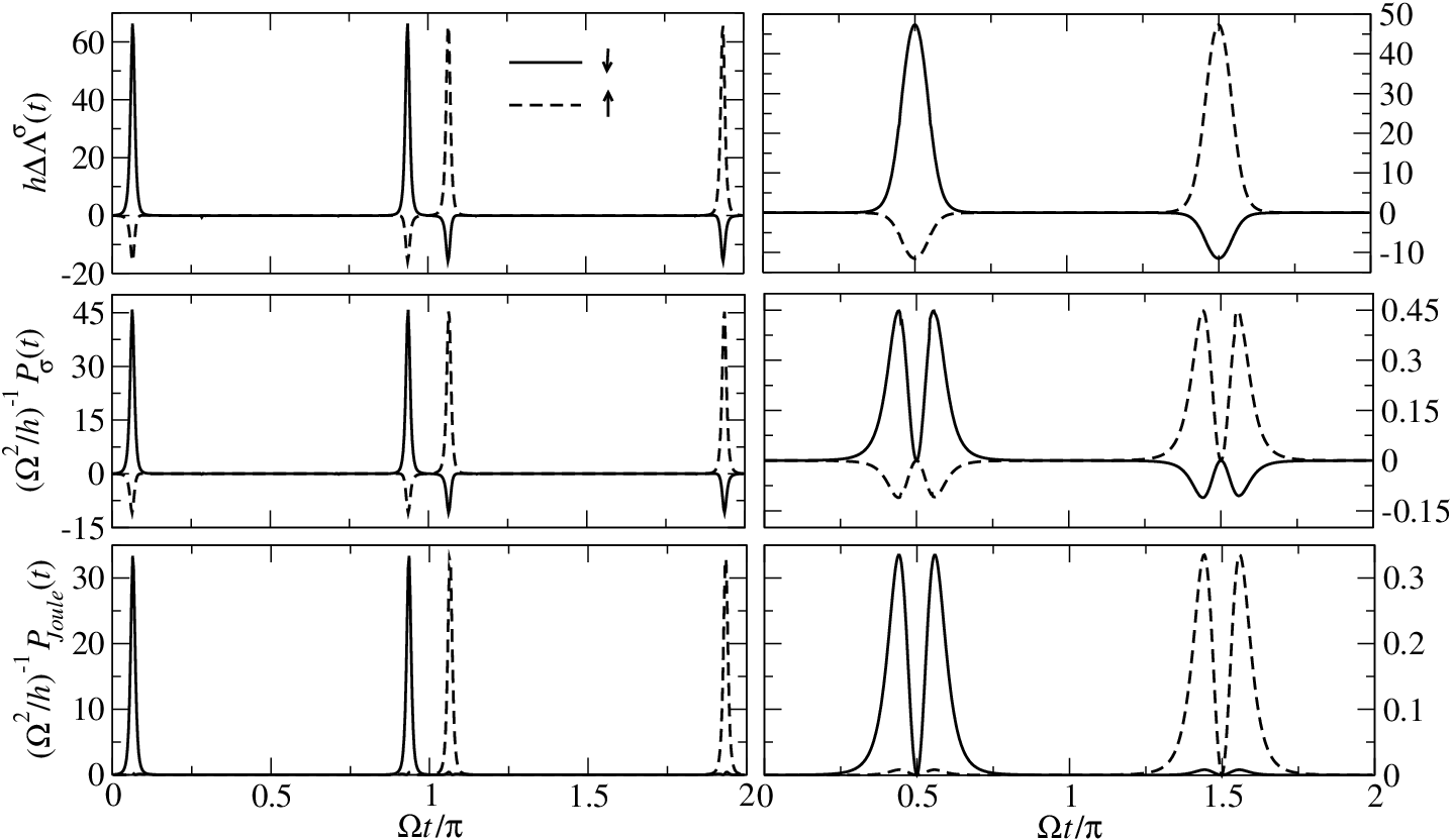
The behavior of the coefficients $\Lambda_{\sigma}$, which determine the non-conservative component of the power, is illustrated in Fig. 8 for the largest value of $U$ shown in Fig. 7. These coefficients display a very interesting behavior as functions of time. Both exhibit features at those times where the occupancy of the quantum dot experiences a significant fluctuation, implying a finite charge current flowing between the reservoir and the quantum dot. The coefficient $\Lambda_{\downarrow}(t)$, associated to electrons with the majority spin polarization is always positive in the interval of time shown. Note that the symmetry transformation Eq. (27) implies that $\Lambda_{\uparrow}(t)=\Lambda_{\downarrow}(-t)$. Instead, the coefficient $\Lambda_{\uparrow}(t)$, which is related to the minority spin orientation can be negative. Notice that this is in strong contrast to the non-polarized case, where the two coefficients are identical and positive. The coefficients $\Lambda_{\sigma}(t)$ do not separately satisfy the Korringa-Shiba law of the non-interacting system expressed by Eq. (18). This can be seen by comparing the plots in symbols with those in lines in the upper panel of the figure. However, the total coefficient $\Lambda^{c}(t)$ obeys the Korringa-Shiba relation (19), as shown in the bottom panel of the figure.

The corresponding behavior of the developed power is presented in Fig. 9 for the smallest and largest value of $U$ considered in Fig. 7. We show in the upper panels the coefficients $\Lambda_{\sigma}(t)$, and in the middle panels the corresponding non-conservative powers $P_{\sigma}(t)$. Note that $P_{\uparrow}(t)=-P_{\downarrow}(-t)$ as a consequence of the symmetry transformation Eq. (27). For comparison, the lower panels show the IJL per spin, $P_{\rm Joule,\sigma}(t)$. All these quantities have features at those times $t$ where the occupancy of the dot changes and a charge current is established between the dot and the reservoir.

As mentioned in the discussion of the previous figure, the striking feature is the different sign of $\Lambda_{\downarrow}(t)$ and $\Lambda_{\uparrow}(t)$, and the consequent opposite sign of the powers $P_{\downarrow}(t)$ and $P_{\uparrow}(t)$. This means that the contributions of different spin to the total power do not separately dissipate heat in the form of a Joule law, as is the case of the unpolarized quantum dot but they can be decomposed as $P_{\sigma}(t)=\xi_{\sigma}P_{\rm ex}(t)+P_{\rm Joule,\sigma}(t)$, with $\xi_{\sigma}=\pm$. Here, the component $P_{\rm Joule,\sigma}(t)$ is associated to the energy dissipated in the form of heat. Instead, $P_{\rm ex}(t)$ is associated to energy that is transferred in the form of work done by the electrons with the minority spin component on the electrons with the majority spin component or vice versa. The total dissipated power is given by the addition of the Joule components, which is shown in the lower panels of the figure. The mechanism of energy exchange leading to $P_{\rm ex}(t)$ is a consequence of the combined effect of many-body interactions and the spin polarization due to the magnetic field. In fact, we stress that in the non-interacting case with $U=0$, $P_{\rm ex}(t)=0$, as shown in Section III B.

To understand the fundamental difference between the non-interacting and interacting case, let us notice that in the non-interacting case, electrons with the two spin components behave independently one another. Due to the Zeeman splitting there is one energy level for electrons with $\uparrow$ spin and one for electrons with $\downarrow$ spin, which are rigidly shifted upwards and downwards in energy as the gate voltage changes. Every time that one of these levels gets aligned with the Fermi energy of the reservoir, the occupancy of the quantum dot changes and a current sets between the quantum dot and the reservoir. Such process is accompanied by Joule heating in the form of $P_{\rm Joule,\sigma}(t)$ with resistance $R_{0}$. Instead, in the interacting regime, the single occupancy is dominated by spins aligned with the magnetic field, while in the configurations with 0 and 2 electrons in the quantum dot, both spin orientations are equally populated. For this reason, when the occupancy changes from singly to double occupancy, there is a flux of spins oriented opposed to the magnetic field following the gate voltage, along with a smaller counter flow of electrons aligned with the magnetic field against the gate voltage. Analogous situations take place when the configuration changes from double to single occupancy and from single occupancy to the empty configuration. The energy to generate the current of the electrons with one of the spin components that opposes to the direction dictated by the external gate voltage is provided by the electrons with the opposite spin component. This is precisely what we have discussed within the RPA approximation in Section IV. C. In a full cycle, this energy exchange averages to zero and only the Joule dissipation remains.

In Fig. 10 we represent the average power over the cycle for a given spin ${\bar{P}}_{\sigma}$. As a consequence of the symmetry transformation Eq. (27) for the chosen parameters, ${\bar{P}}_{\downarrow}={\bar{P}}_{\uparrow}$. We also represent in the figure the components ${\bar{P}}_{\uparrow\uparrow}$ and ${\bar{P}}_{\uparrow\downarrow}$, which correspond to the contributions of the same and opposite spin to the average total power for spin up, according to Eqs. (9), (10) and (11). One can see that the crossed component ${\bar{P}}_{\uparrow\downarrow}$, which vanishes for $U=0$, decreases rapidly as $U$ is turned on and saturates when $U$ reaches values much larger than both $\Delta$ and the Zeeman splitting $\delta_{Z}$. Instead, for small $U$, ${\bar{P}}_{\uparrow\uparrow}$ increases but nos so fast s the decrease in ${\bar{P}}_{\uparrow\downarrow}$, so that the sum ${\bar{P}}_{\uparrow}$ decreases for small $U$.

For larger values of $U$ after a modest increase, ${\bar{P}}_{\sigma}$ decreases because the charge-transfer peaks in the spectral density (separated by $U$) cross the Fermi level with a smaller speed, so that the factor $\dot{V}_{g}(t)^{2}$ is smaller [see Eq. (20)] and when $U$ becomes larger than $2V_{0}$, the charge-transfer peaks cannot cross the Fermi energy during the cycle and the power drops to zero.

References

- [1] J. Gabelli, G. Fève, J.-M. Berroir, B. Placais, A.Cavanna, E.al,Y. Jin, and D. C. Glattli, Science 313, 499 (2006).
- [2] G. Fève, A. Mahé, J.-M. Berroir, T. Kontos, B. Placais, C. Glattli, A. Cavanna, B. Etienne, and Y. Jin, Science 316, 1169 (2007).
- [3] J. Gabelli, G. Féve, J.-M. Berroir, and B. Placais, Rep. Prog. Phys. 75, 126504 (2012).
- [4] M. Büttiker, A. Prêtre, and H. Thomas, Phys. Rev. Lett. 70, 4114 (1993).
- [5] A. Prêtre, H. Thomas, and M. Büttiker, Phys. Rev. B 54, 8130 (1996).
- [6] M. Büttiker, H. Thomas, and A. Prêtre, Phys. Lett. A 180, 364 (1993).
- [7] S. E. Nigg, R. López, and M. Büttiker, Phys. Rev. Lett. 97, 206804 (2006).
- [8] M. Lee, R. López, M.-S. Choi, T. Jonckheere, and T. Martin, Phys. Rev. B 83, 201304 (2011).
- [9] C. Mora and K. Le Hur, Nat. Phys. 6, 697 (2010).
- [10] M. Filippone, K. Le Hur, and C. Mora, Phys. Rev. Lett. 107, 176601 (2011).
- [11] M. Filippone, C. Mora, Phys. Rev. B 86, 125311 (2012).
- [12] M. Moskalets, P. Samuelsson, and M. Büttiker Phys. Rev. Lett. 100, 086601 (2008).
- [13] S. Okhovskaya, J. Splettstoesser, M. Moskalets, and M. Büttiker, Phys. Rev. Lett. 101, 166802 (2008).
- [14] J. Splettstoesser, M. Moskalets, and M. Büttiker, Phys. Rev. Lett. 103, 076804 (2009).
- [15] Géraldine Haack, Michael Moskalets, Markus Büttiker Phys. Rev. B 87, 201302(R) (2013).
- [16] O. Kashuba, H. Schoeller, J. Splettstoesser, Eur. Phys. Lett. 98, 57003 (2012).
- [17] M. I. Alomar, J. S. Lim, and David Sánchez, Phys. Rev. B 94, 165425 (2016).
- [18] D. Litinski, P. W. Boruwer, and M. Filippone, arXiv:1612.04822.
- [19] M. F. Ludovico, J. S. Lim, M. Moskalets, L. Arrachea and D. Sánchez, Phys. Rev. B 89, 161306(R) (2014).
- [20] L. Arrachea, M. Moskalets and L. Martin-Moreno, Phys. Rev. B 75 245420 (2007).
- [21] M. F. Ludovico, M. Moskalets, D. Sánchez, and L. Arrachea, Phys. Rev. B 94, 035436 (2016).
- [22] Notice that this definition is consistent with , where is the internal energy of the electron system (assumed to remain constant for the full system containing the dot and the reservoir).
- [23] A. C. Hewson, ”The Kondo Problem to Heavy Fermions” (Cambridge University Press, Cambridge, 1993).
- [24] M.F. Ludovico, F. Battista, F. von Oppen and L. Arrachea, Phys. Rev. B 93, 075136 (2016).
- [25] J-T. Lü, M. Brandbyge and P. Hedegard, Nano Lett. 10 1657 (2010).
- [26] H. Shiba, Prog. of Theor. Phys. 54, 967 (1975).
- [27] L. Arrachea, Phys. Rev. B 72, 125349 (2005); ibid 75, 035319 (2007).
- [28] P. B Wiegmann and A. M. Tsvelick, J. Phys. C 16, 2281 (1983).
- [29] I. J. Hamad, P. Roura-Bas, A. A. Aligia, and E. V. Anda, Physica Status Solidi (b) 253, 478 (2015).
- [30] R. Žitko, NRG LJUBLJANA , open source numerical renormalization group code, http://nrgljubljana.ijs.si
- [31] A. A. Aligia, P. Roura-Bas, and S. Florens, Phys. Rev. B 92, 035404 (2015); references therein.
- [32] M. M. Desjardins, J. J. Viennot, M. C. Dartiailh, L. E. Bruhat, M. R. Delbecq, M. Lee, M.-S. Choi, A. Cottet, and T. Kontos, Nature 545, 71 (2017).
- [33] V.L. Campo and L.N. Oliveira, Phys. Rev. B 72, 104432 (2005).
- [34] M. Yoshida, M. A. Whitaker, and L. N. Oliveira, Phys. Rev. B 41, 9403 (1990).
- [35] R. Bulla, T. A. Costi, and T. Pruschke, Rev. Mod. Phys. 80, 395 (2008).
- [36] Z. Osolin, and R. Žitko, Physical Review B 87, 245135 (2013).
- [37] M. Kataoka, C. J. B. Ford, M. Y. Simmons, and D. A. Ritchie Phys. Rev. Lett. 89, 226803 (2002).
- [38] H.-S. Sim, M. Kataoka, C.J.B. Ford, Phys. Rep. 456, 127 (2008).
- [39] S. Gasparinetti, K. L. Viisanen, O.-P. Saira, T. Faivre, M. Arzeo, M. Meschke, and J. P. Pekola Phys. Rev. Applied 3, 014007 (2015).
- [40] M. Zgirski, M. Foltyn, A. Savin, M. Meschke, J. Pekola, arXiv:1704.04762.