On the analytical properties of the magneto-conductivity in the case of presence of stable open electron trajectories on a complex Fermi surface.

Our considerations here will be connected with the geometry of the quasiclassical electron trajectories on the Fermi surface in the presence of a strong magnetic field. The main goal of the paper is to give a detailed consideration of the contribution of the stable open trajectories to the conductivity tensor in the limit $\,\omega_{B}\tau\,\rightarrow\,\infty$. As we will see below, in spite of rather regular geometric properties of the stable (generic) open trajectories, their contribution to magneto-conductivity is quite non-trivial from analytical point of view, which is caused by nontrivial statistical properties of the trajectories of this kind. Here we will try to represent a general picture of the magneto-conductivity behavior in the case of presence of such trajectories on the Fermi surface, including the description of the dependence of conductivity on both the magnitude and the direction of $\,{\bf B}$. As we will see, both the structure of a “Stability Zone” on the angle diagram and the conductivity behavior in strong magnetic fields will demonstrate actually rather non-trivial properties.

We will base our considerations on the topological picture for the electron dynamics in the space of the quasimomenta, arising for general dispersion relation $\,\epsilon({\bf p})\,$ under the presence of a magnetic field. So, according to standard approach we will assume that the electron states in the conduction band are parametrized by the values of the quasimomenta ${\bf p}$ which in fact should be considered as points of the three-dimensional space, factorized over the vectors of the reciprocal lattice:

The basis vectors of the reciprocal lattice are connected with the basis vectors $\,({\bf l}_{1},\,{\bf l}_{2},\,{\bf l}_{3})\,$ of the direct lattice by the formulae

and define the fundamental (Brillouen) zone in the $\,{\bf p}$ - space.

The opposite faces of the parallelepiped formed by $\,({\bf a}_{1},\,{\bf a}_{2},\,{\bf a}_{3})\,$ should be identified with each other, so the space of the electron states (for a given conduction band) represents in fact the three-dimensional torus $\,\mathbb{T}^{3}$.¹¹ 1 We do not consider here the spin variables, which will not play an essential role in our picture.

The dispersion relation $\,\epsilon({\bf p})\,$ can be considered either as a 3-periodic function in the $\,{\bf p}$ - space or just as a smooth function on the compact manifold $\,\mathbb{T}^{3}$, given by the factorization of the $\,{\bf p}$ - space over the reciprocal lattice $\,L$. In the same way, the constant energy levels $\,\epsilon({\bf p})\,=\,{\rm const}\,$ can be considered either as 3-periodic two-dimensional surfaces in the $\,{\bf p}$ - space or as smooth compact surfaces $\,S_{\epsilon}\,\subset\,\mathbb{T}^{3}\,$ embedded in the three-dimensional torus $\,\mathbb{T}^{3}$. Being considered in the last way, every nonsingular energy level represents a smooth compact orientable surface, which is topologically equivalent to one of the canonical surfaces defined by genus $g$ (Fig. 1).

The genus $\,g\,$ of the Fermi surface represents an important topological characteristic of the electron spectrum in metal. Another important topological characteristic of the electron spectrum is the way of embedding of the Fermi surface in $\,\mathbb{T}^{3}$. As an example, Fig. 2   represents an embedding of a genus 3 surface in the first Brillouen zone having ‘‘maximal rank’’.

The quasiclassical evolution of the electron states in the presence of external homogeneous magnetic field ${\bf B}$ can be described by the adiabatic equation (see e.g. [16, 35]):

in the space of the quasimomenta.

The equation (I.1) is analytically integrable in $\,{\bf p}$ - space and the quasiclassical trajectories are given by the intersections of the constant energy surfaces $\,\epsilon({\bf p})\,=\,{\rm const}\,$ with the planes orthogonal to $\,{\bf B}$. However, despite this analytical property of system (I.1), the global geometry of the quasiclassical trajectories in $\,{\bf p}$ - space can be rather complicated. The reason for this circumstance is that the total ${\bf p}$ - space is not compact while in $\,\mathbb{T}^{3}\,$ the function $\,\epsilon({\bf p})\,$ represents the only one-valued integral of motion of (I.1). In general, we can expect rather complicated picture of intersection of the 3-periodic surface $\,\epsilon({\bf p})\,=\,{\rm const}\,$ with the planes orthogonal to general (totally irrational) direction of $\,{\bf B}\,$ (see e.g. Fig. 3).

As it is usual for the case of normal metals, we will assume here that all the electron states with energies below the Fermi energy $\,\epsilon_{F}\,$ are occupied by electrons, while all the electron states with energies above the Fermi energy are empty. The Fermi surface $\,\,S_{F}:\,\,\epsilon({\bf p})\,=\,\epsilon_{F}\,$ represents a two-dimensional surface in $\,\mathbb{T}^{3}\,$ separating occupied electron states from the empty ones. We have naturally $\,\epsilon_{\rm min}\,<\,\epsilon_{F}\,<\,\epsilon_{\rm max}\,$ where $\,\epsilon_{\rm min}\,$ and $\,\epsilon_{\rm max}\,$ are the minimal and maximal possible electron energies in the conductivity zone.

System (I.1) conserves the energy of a particle and also the phase volume element $\,d^{3}p$. As a consequence, the evolution according to system (I.1) does not change the Fermi distribution of the quasiparticles or more general temperature dependent equilibrium distributions

However, it appears that the form of the trajectories of (I.1) plays an important role for the response of the electron system to the small electric fields $\,{\bf E}$, which defines the magneto-conductivity properties of normal metals. Due to the high degeneracy of the electron gas in metals, all the properties of such transport phenomena are defined in fact by the properties of system (I.1) just on the one energy level $\,\epsilon\,=\,\epsilon_{F}\,,\,\,$ i.e. just on the one (Fermi) energy surface $\,\epsilon({\bf p})\,=\,\epsilon_{F}$.

The role of the global geometry of the quasiclassical electron trajectories in the transport phenomena in strong magnetic fields was first revealed by the school of I.M. Lifshitz (I.M. Lifshitz, M.Ya. Azbel, M.I. Kaganov, V.G. Peschansky) in 1950’s (see [17, 18, 19, 20, 21, 23]). Thus, in paper [17] a crucial difference in contribution to magneto-conductivity of closed (Fig. 4, a) and open periodic (Fig. 4, b) quasiclassical trajectories in the limit $\,B\,\rightarrow\,\infty\,$ was pointed out.

As was shown in [17], the contribution to the magneto-conductivity of the trajectories of the first kind is almost isotropic in the plane orthogonal to $\,{\bf B}\,$ and has a rapidly decreasing character in this plane as $\,B\,\rightarrow\,\infty$. In contrast, the presence of the open periodic trajectories gives an additional contribution to the conductivity in the plane orthogonal to $\,{\bf B}$, which is strongly anisotropic in the limit $\,B\,\rightarrow\,\infty$. The asymptotic form of the conductivity tensor in the plane orthogonal to $\,{\bf B}\,$ in the described cases can be represented as

(closed trajectories),

(open periodic trajectories), after an appropriate choice of coordinates. (Here and below the notation $\,*\,$ means just a constant of the order of unity).

The formulae (I.2) - (I.3) represent the asymptotic form of the conductivity tensor, so all the equalities give actually just the order of the absolute value of the corresponding quantities.

The value $\,m^{*}\,$ represents here just some (approximate) effective mass of electron in crystal and $\,\tau\,$ denotes the mean free electron time defined by the intensity of the scattering processes.

The value

can be considered as an “approximate value” of the cyclotron frequency in the crystal. From geometrical point of view $\,\omega_{B}\,$ represents approximately the inverse time of motion along a closed trajectory (Fig. 4, a) or the inverse time of motion through one Brillouen zone for periodic open trajectories (Fig. 4, b). It becomes clear from this point of view that the global geometry of the quasiclassical trajectories reveals exactly in the limit $\,\omega_{B}\tau\,\rightarrow\,\infty\,$ when the mean free electron time exceeds the time of motion inside one Brillouen zone. Let us say here that for experimental observation of the “geometric strong magnetic field limit” rather pure materials under rather low temperatures ($T\,\sim\,1K$) and rather strong magnetic fields ($B\,\sim\,10^{4}\,Gs$) should be usually used.

In formula (I.3) the $\,x$ - axis is chosen along the mean direction of the periodic trajectories in $\,{\bf p}$ - space. As can be easily derived from system (I.1), the projection of the corresponding trajectory in coordinate space onto the plane orthogonal to $\,{\bf B}\,$ is given just by the rotation of the trajectory in $\,{\bf p}$ - space by $90^{\circ}$ (Fig. 5).

We can see then that even very strong magnetic field does not block the electron motion along the $\,y$ - axis in the coordinate space in the presence of the trajectories shown at Fig. 4, b. As a result, the $\,y$ - component of conductivity in the plane orthogonal to $\,{\bf B}\,$ remains finite in the limit $\,\omega_{B}\tau\,\rightarrow\,\infty$. The strong anisotropy of the conductivity tensor in this situation gives an experimental possibility to observe this phenomenon as well as to determine the mean direction of the open trajectories in $\,{\bf p}$ - space.

The conductivity along the direction of $\,{\bf B}\,$ remains finite in the limit $\,\omega_{B}\tau\,\rightarrow\,\infty\,$ in both the cases described above. The asymptotic forms of the full conductivity tensor in $\,{\bf x}$ - space can be represented as:

(closed trajectories),

(open periodic trajectories).

Let us note here that both the trajectories shown at Fig. 4   are actually closed in the torus $\,\mathbb{T}^{3}$. However, their embeddings in $\,\mathbb{T}^{3}\,$ are completely different from topological point of view. Thus, the embedding of the trajectory shown at Fig. 4, a   is ‘‘homologous’’ to zero, while the embedding of the trajectory shown at Fig. 4, b   represents a nonzero homology class in $\,\mathbb{T}^{3}$. Certainly, the difference between the trajectories shown at Fig. 4, a   and   Fig. 4, b   is more evident in the covering ${\bf p}$ - space where they have different global geometry.

Let us say here also, that both the situations shown at Fig. 4 a,b   represent the special case when the conductivity tensor can be represented as a regular series in powers of $\,(\omega_{B}\tau)^{-1}\,$ in the limit $\,\omega_{B}\tau\,\rightarrow\,\infty$. Thus, we can actually write here

(closed trajectories),

(open periodic trajectories), where the even powers of $\,\omega_{B}\tau\,$ correspond to the symmetric part of $\,\sigma^{kl}(B)\,$, while the odd powers of $\,\omega_{B}\tau\,$ represent the anti-symmetric part in accordance with the Onsager relations.

As we will see below, this situation does not take place for general open electron trajectories on the Fermi surface.

In papers [18, 19] different examples of complicated Fermi surfaces and more general types of open electron trajectories in strong magnetic fields were considered. The trajectories considered in [18, 19] are in general not periodic and are non-closed both in $\,\mathbb{T}^{3}\,$ and the ${\bf p}$ - space and represent the first examples of the stable open electron trajectories on a complicated Fermi surface. The form of the trajectories found in [18, 19] demonstrates also strongly anisotropic properties, so the strong anisotropy of the conductivity tensor in the limit $\,\omega_{B}\tau\,\rightarrow\,\infty\,$ is also expected in this case. As was pointed out in [15], the analytical behavior of conductivity in these examples can in fact be different from (I.5) and demonstrate a slower approach to its limiting form in the interval of not extremely strong magnetic fields. Here we will try to study this question in general case using the topological description of the stable open trajectories on the Fermi surface.

In the survey articles [20, 21, 22] and also in the book [23] a remarkable review of both the theoretical and experimental investigations of this branch of electron theory of metals made at that time can be found. Let us give here also a reference on a survey article [15] where the same topics were revisited after forty years and which contains also the aspects appeared in the later period.

The general problem of classification of all possible types of trajectories of dynamical system (I.1) with arbitrary (periodic) dispersion law $\,\epsilon({\bf p})\,$ was set by S.P. Novikov ([27]) and was intensively investigated in his topological school (S.P. Novikov, A.V. Zorich, S.P. Tsarev, I.A. Dynnikov). The topological investigation of system (I.1) has led to rather detailed understanding of the geometry of the trajectories of different types and gave finally the full classification of all possible types of trajectories of (I.1). One of the most important parts of the mathematical theory of the trajectories of (I.1), which will be also of great importance in the present paper, is connected with the detailed description of the stable open trajectories of system (I.1). Let us say here that the most important breakthroughs in this problem were made in papers [36, 8] where rather deep topological theorems about non-closed trajectories of system (I.1) were proved.

Using the topological description of the stable open trajectories of system (I.1) it was possible to introduce important topological characteristics of the stable nontrivial regimes of the magneto-conductivity behavior in the limit $\,\omega_{B}\tau\,\rightarrow\,\infty\,$, which were introduced in paper [28]. In general, the characteristics introduced in [28] can be described in the following way:

Let us exclude now the “trivial” cases when we have just closed electron trajectories on the Fermi surface in ${\bf p}$ - space and consider the situation when open trajectories (in ${\bf p}$ - space) are present on the Fermi level. Besides that, let us require that the open trajectories are stable with respect to small rotations of $\,{\bf B}\,$ such that we have a “Stability Zone” in the space of directions of $\,{\bf B}$, where similar open trajectories exist on the Fermi level.

As can be extracted from the topological description of the stable open trajectories of system (I.1), the trajectories of this type demonstrate the following remarkable properties:

1) Every stable open (in ${\bf p}$ - space) trajectory of (I.1) lies in a straight strip of a finite width in the plane orthogonal to $\,{\bf B}$, passing through it from $\,-\infty\,$ to $\,+\infty\,$ (Fig. 6);

2) The mean direction of all open stable trajectories in ${\bf p}$ - space is given by the intersection of the plane orthogonal to $\,{\bf B}\,$ and some integral (generated by two reciprocal lattice vectors) plane $\,\Gamma$, which is the same for a given “Stability Zone” in the space of directions of $\,{\bf B}$.

Let us note here that the statement (1) was first formulated by S.P. Novikov in the form of a conjecture, which was proved later for the stable open trajectories of (I.1) ([36, 8]).

As was pointed out in [28], the integral planes $\,\Gamma_{\alpha}\,$ represent experimentally observable objects view the remarkable geometric properties of the open stable trajectories, described above. Thus, measuring the conductivity in the limit $\,\omega_{B}\tau\,\rightarrow\,\infty$, we can observe strongly anisotropic behavior of conductivity in the planes orthogonal to $\,{\bf B}\,$ for all $\,{\bf B}/B\,\in\,\Omega_{\alpha}\,$ and extract the integral plane $\,\Gamma_{\alpha}$, which is swept by the directions of the highest decreasing of conductivity in the ${\bf x}$ - space.

More precisely, let us introduce the values

Then, we can chose a basis in ${\bf x}$ - space

smoothly depending on $\,{\bf B}\,$ in $\,\Omega_{\alpha}$, where the values $\,\sigma^{kl}_{\infty}\,$ will have the form

As was said above, the direction of the vector $\,{\bf e}_{1}({\bf B})\,$ is given by the intersection of the plane orthogonal to $\,{\bf B}\,$ with an integral plane, i.e. the plane generated by two reciprocal lattice vectors $\,{\bf q}_{1}$, $\,{\bf q}_{2}$, which is the same for the Zone $\,\Omega_{\alpha}$.

The integral plane $\,\Gamma_{\alpha}\,$ can be represented by an indivisible triple of integer numbers $\,(M^{1}_{\alpha},\,M^{2}_{\alpha},\,M^{3}_{\alpha})\,$ according to the equation

where $\,({\bf l}_{1},\,{\bf l}_{2},\,{\bf l}_{3})\,$ are the basis direct lattice vectors. The numbers $\,(M^{1}_{\alpha},\,M^{2}_{\alpha},\,M^{3}_{\alpha})\,$ were called in [28] the topological quantum numbers observable in conductivity of normal metals. Let us say here that the triples $\,(M^{1}_{\alpha},\,M^{2}_{\alpha},\,M^{3}_{\alpha})\,$ can be rather nontrivial for complicated Fermi surfaces.

The complete Zone $\,\Omega_{\alpha}\,$ can be called here the mathematical Stability Zone, corresponding to a given Fermi energy. We have to say here, however, that in experimental study of magneto-conductivity it is natural to introduce extended “experimentally observable Stability Zone” $\,\,\hat{\Omega}_{\alpha}\,\,$ $(\Omega_{\alpha}\subset\hat{\Omega}_{\alpha})\,\,$ due to specific behavior of trajectories of system (I.1) near the boundary of $\,\Omega_{\alpha}$. Everywhere in $\,\hat{\Omega}_{\alpha}\,$ the behavior of conductivity is experimentally indistinguishable from that in $\,\Omega_{\alpha}\,$ even under good formal implementation of the condition $\,\omega_{B}\tau\,\gg\,1\,$ until the magnitude $\,B\,$ of magnetic field becomes extremely high. The conventional form of $\,\hat{\Omega}_{\alpha}\,$ depends actually on the experimental conditions and is determined mainly by the maximal values of $\,B\,$ in experiment. The difference between the Zones $\,\hat{\Omega}_{\alpha}\,$ and $\,\Omega_{\alpha}$, which can be detected only in extremely strong magnetic fields, represents in fact one of essential features of analytical behavior of conductivity, considered here.

Let us note now that the stable open quasiclassical trajectories do not represent all possible types of non-closed trajectories of system (I.1) and trajectories with more complicated geometry can arise on complicated Fermi surfaces for some special directions of $\,{\bf B}$. Thus, the first example of trajectory which can not be restricted by any straight strip of a finite width was constructed by S.P. Tsarev ([34]). The trajectory of Tsarev demonstrates explicit chaotic behavior on the Fermi surface and is essentially different from the stable open trajectories from this point of view. On the other hand, the Tsarev trajectory is also strongly anisotropic in the ${\bf p}$ - space and has an asymptotic direction in the plane orthogonal to $\,{\bf B}$. So, from experimental point of view the contribution of Tsarev trajectories to the magneto-conductivity is also strongly anisotropic in the limit $\,\omega_{B}\tau\,\rightarrow\,\infty\,$ and corresponds to the regime (I.8). Let us say, however, that the Tsarev chaotic trajectories are completely unstable under small rotations of $\,{\bf B}\,$ and are not connected with topologically stable characteristics unlike the stable open trajectories discussed above. We have to say also, that the trajectories of Tsarev type (if they present) can appear just for the set of zero measure in the space of directions of $\,{\bf B}$.

Another example of non-closed trajectory of (I.1) which demonstrates strongly chaotic behavior both in $\,\mathbb{T}^{3}\,$ and in ${\bf p}$ - space was constructed by I.A. Dynnikov in [9]. The trajectories of Dynnikov are rather different from the Tsarev chaotic trajectories and require the maximal irrationality of the direction of $\,{\bf B}\,$ to be observed. The behavior of the conductivity tensor in the presence of the chaotic trajectories constructed in [9] was investigated in [24] and appeared to be rather different from both the regimes given by (I.4) and (I.5). The most interesting feature of the contribution to the conductivity tensor of the trajectories of this kind is that the presence of such trajectories suppresses the conductivity in all directions, including the direction of $\,{\bf B}$, in the limit $\,\omega_{B}\tau\,\rightarrow\,\infty$.

In general, the Tsarev and Dynnikov chaotic trajectories demonstrate two different general types of possible chaotic behavior of trajectories of system (I.1), so in this sense all chaotic trajectories of (I.1) can be attributed to the Tsarev or Dynnikov type. Let us say here that different properties of chaotic trajectories of system (I.1) are also intensively investigated in modern mathematical literature (see [37, 10, 3, 4, 5, 6, 11, 7, 32, 33, 12]).

The directions of $\,{\bf B}\,$, corresponding to the chaotic open trajectories, can appear only outside the “Stability Zones”, corresponding to the stable open trajectories of system (I.1). In the same way, the chaotic open trajectories of different types (Tsarev or Dynnikov type) can not appear at the same direction of $\,{\bf B}$. Let us say, however, that in general the contribution of non-closed trajectories to the conductivity tensor should be added with the contribution (I.4) of closed trajectories of system (I.1), which usually present together with open trajectories (of any kind) at the same Fermi surface.

For more rigorous description of possible situations in the behavior of trajectories of (I.1) with arbitrary periodic dispersion law let us give here a reference to a detailed mathematical survey [10], devoted to this question. The detailed consideration of different physical results based on the results of topological investigations of system (I.1) can be found in [29, 25, 26].

Our main goal in this paper will be more detailed investigation of the conductivity behavior in the “Stability Zones”, based on the detailed topological description of the stable open electron trajectories arising for the corresponding directions of $\,{\bf B}$. As we said already, the corresponding stable open trajectories demonstrate rather regular geometric properties in the planes orthogonal to $\,{\bf B}\,$. Thus, all the stable open trajectories have the form shown at Fig. 6 and the same mean direction in $\,{\bf p}$ - space, given by the intersection of the plane orthogonal to $\,{\bf B}\,$ with an integral plane $\,\Gamma_{\alpha}$, which is fixed for the corresponding Stability Zone $\,\Omega_{\alpha}$. As a result, the conductivity tensor has the asymptotic form (I.8) in the limit $\,\omega_{B}\tau\,\rightarrow\,\infty\,$ and demonstrates the specific geometric properties described above. These geometric (or topological) properties of the conductivity tensor give the most stable (topological) characteristics of the conductivity for a given “Stability Zone” and are connected with the “purely geometric” limit $\,\omega_{B}\tau\,\rightarrow\,\infty$. At the same time, we will see below, that the conductivity tensor demonstrates in general rather nontrivial analytical dependence on $\,{\bf B}\,$ in different parts of “experimentally observable” Stability Zones, which is caused by specific features of different trajectories of system (I.1) in these regions. Here we will investigate the analytical properties of conductivity for the case of rather big (but finite) values of the parameter $\,\omega_{B}\tau\,$ using topological description of “carriers of open trajectories” on the Fermi surface, defined for the corresponding directions of $\,{\bf B}$. As we will see below, both the dependence on the parameter $\,\omega_{B}\tau\,$ and on the direction of $\,{\bf B}\,$ demonstrate here rather nontrivial properties.

In the next section we will give a description of “experimentally observable” Stability Zone and try to describe the main features of the analytical behavior of conductivity in its different parts, which gives from our point of view the main points of the picture arising in general case. In Sections III and IV we will present more detailed consideration of the contribution of the stable open trajectories to the magneto-conductivity, based on the topological description of such trajectories on complicated Fermi surfaces. Sections III and IV will have more mathematical character in comparison with Section II.

To describe briefly the general picture, let us point out now the main points, which will play the most essential role in our considerations below. This section will be mostly descriptive, while more detailed analysis will be presented in Sections III, IV.

As we said already, the stable open trajectories demonstrate quasiperiodic properties for generic directions of $\,{\bf B}\,\,$ (${\bf B}/B\,\in\,\Omega_{\alpha}$). However, they become purely periodic for some special directions of the magnetic field. It’s not difficult to see that the last situation arises every time when the plane orthogonal to $\,{\bf B}\,$ intersects the plane $\,\Gamma_{\alpha}\,$ along an integer vector in ${\bf p}$ - space:

($k_{1},\,k_{2},\,m_{1},\,m_{2},\,m_{3}\,\,\in\,\,\mathbb{Z}$).

Both the cases of the quasiperiodic and the periodic trajectories lead in this situation to the conductivity tensor (I.8) in the limit $\,\omega_{B}\tau\,\rightarrow\,\infty$, having the same stable geometric properties for a given “Stability Zone”. However, as we will see below, the limiting values of the components $\,\sigma^{22}$, $\,\sigma^{23}$, $\,\sigma^{32}$, $\,\sigma^{33}$,   i.e. the values

(${\bf B}/B\,$ is fixed), will have here sharp “jumps” with respect to the same values, defined for close generic directions of $\,{\bf B}$.

More precisely, we can introduce the functions $\,\,{\bar{\sigma}}^{kl}_{\infty}\,({\bf B}/B)\,$, $\,\,(k,l\,=\,2,3)\,,\,$ which represent continuous functions of $\,\,{\bf n}\,=\,{\bf B}/B\,$ in $\,\Omega_{\alpha}\,$ and coincide with the corresponding values $\,\sigma^{kl}_{\infty}\,({\bf B}/B)\,$ for generic directions $\,{\bf B}/B\,\in\,\Omega_{\alpha}$. However, for special directions of $\,{\bf B}\,$ described above we will have $\,\,\sigma^{kl}_{\infty}\,({\bf B}/B)\,\neq\,{\bar{\sigma}}^{kl}_{\infty}\,({\bf B}/B)\,,\,\,$ which is caused by special features of statistical averaging over the open trajectories of (I.1) near the Fermi surface. It’s not difficult to show also that we will always have the inequalities

for these special directions of $\,{\bf B}$, while the signs of $\,\,\,\sigma^{kl}_{\infty}\,({\bf B}/B)\,\,-\,\,{\bar{\sigma}}^{kl}_{\infty}\,({\bf B}/B)\,\,,\,\,\,k\,\neq l\,,\,\,\,$ are in general indefinite.

The directions $\,{\bf B}/B\,\in\,\Omega_{\alpha}$, corresponding to a fixed rational mean direction $\,{\bf a}\,$ of open trajectories, represent a one-dimensional curve $\,\gamma^{\alpha}_{\bf a}\,$ (on $\,\mathbb{S}^{2}$) given by the intersection of the big circle, orthogonal to $\,{\bf a}$, and the Stability Zone $\,\Omega_{\alpha}\,$ (Fig. 7 a). We have to say, however, that according to a more detailed consideration the periodic trajectories exist actually on some bigger curve $\,{\hat{\gamma}}^{\alpha}_{\bf a}\,$ representing extension of the curve $\,\gamma^{\alpha}_{\bf a}\,$ outside the Stability Zone $\,\Omega_{\alpha}\,$ (Fig. 7 b). All the open trajectories have the same mean direction $\,{\bf a}\,$ for all $\,{\bf B}/B\,\in\,{\hat{\gamma}}^{\alpha}_{\bf a}\,$ and the area covered by the periodic trajectories on the Fermi surface vanishes at the endpoints of $\,{\hat{\gamma}}^{\alpha}_{\bf a}$. The open periodic trajectories demonstrate stability properties inside the Stability Zone $\,\Omega_{\alpha}\,$ and become unstable outside $\,\Omega_{\alpha}\,$ on the curve $\,{\hat{\gamma}}^{\alpha}_{\bf a}$. Let us note also here that the measure of generic (quasiperiodic) open trajectories on the Fermi surface remains finite up to the boundary of a Stability Zone. In general, the schematic angle diagram corresponding to a complicated Fermi surface can be represented by Fig. 8.²² 2 We would like to emphasize here that for generic Fermi level $\,\epsilon_{F}\,$ the measure of the stable open trajectories on the Fermi surface remains finite up to the boundary of the “mathematical Stability Zone” $\,\Omega_{\alpha}$. However, it is often assumed in the literature that this measure vanishes at the boundary of a Stability Zone on the angle diagram, which seems to be in accordance with experimental data. As we will see below, the last circumstance is caused by the existence of an extended “experimentally observable” Stability Zone $\,\hat{\Omega}_{\alpha}\,$ including an additional region $\,\Lambda_{\alpha}$, adjacent to the boundary of $\,\Omega_{\alpha}$, with very special behavior of trajectories of system (I.1). It will be also shown, that the presence of additional Zone $\,\Lambda_{\alpha}\,$ is responsible also for arising of rather nontrivial analytical regimes of conductivity behavior in the extended Zone $\,\hat{\Omega}_{\alpha}$.

We can see then that every Stability Zone $\,\Omega_{\alpha}\,$ is actually covered by an everywhere dense net representing the “special directions” of $\,{\bf B}\,$ corresponding to different rational mean directions $\,{\bf a}\,$ of the stable open trajectories (Fig. 9). The set of all possible rational mean directions $\,{\bf a}\,$ of the open trajectories is given by two conditions:

1) $\,{\bf a}\,\,\in\,\,\Gamma_{\alpha}\,\,$,

2) $\,C_{\bf a}\,\cap\,\Omega_{\alpha}\,\,\,\neq\,\,\,\O\,\,$,

Everywhere on the net we have the situation

however, the difference

decreases with the growth of the numbers $\,(m_{1},\,m_{2},\,m_{3})\,$ in (II.1). As we will see below, the approximate evaluation for this difference for complicated Fermi surfaces can be written in the form

($k,l=2,3$).

In the physical situation, when the values of $\,{\bf B}\,$ are finite but rather big, the “jumps” on the curves $\,\gamma^{\alpha}_{\bf a}\,$ become very sharp “peaks” on these curves, which can be called the “rational peaks” in the values of magneto-conductivity according to rationality of the mean direction of the corresponding open trajectories in ${\bf p}$ - space.

The second important point in our picture is connected with the behavior of trajectories of system (I.1) near the boundaries of the Stability Zones $\,\Omega_{\alpha}\,$ outside the Stability Zones. As we have already said, the periodic trajectories of system (I.1) on the Fermi level exist in fact for directions of $\,{\bf B}\,$ belonging to the extended curves $\,{\hat{\gamma}}^{\alpha}_{\bf a}$, so only at the endpoints of $\,{\hat{\gamma}}^{\alpha}_{\bf a}\,$ the measure of the trajectories with the period $\,{\bf a}\,$ on the Fermi surface is equal to zero. As a result, the full set of directions of $\,{\bf B}\,$ near $\,\Omega_{\alpha}\,$, corresponding to the presence of open trajectories on the Fermi level, represents the Stability Zone $\,\Omega_{\alpha}\,$ with a set of additional segments near $\,\Omega_{\alpha}$, which is dense on the boundary of $\,\Omega_{\alpha}\,$ (Fig. 10). ³³ 3 Let us say here that the presence of additional segments adjacent to the Stability Zone on the angle diagram and corresponding to the presence of periodic open trajectories on the Fermi surface was discussed in the literature (see e.g. [18, 19, 20, 21, 22, 23, 15]). It is often assumed, however, that this set is given by a finite number of segments, corresponding to some special (main) rational directions $\,{\bf a}$. As we could find, the first indication of the existence of an everywhere dense set of additional directions of $\,{\bf B}\,$ near the boundary of the zone of stable open trajectories, corresponding to the appearance of periodic trajectories of the system (I.1), was given in the work [13]. Let us say here, that the example in the work [13] is connected with the system (I.1) on a special Fermi surface of genus 2, which are not considered as complex according to our terminology. However, an analogous property is also true in the general case for the Stability Zones on arbitrarily complex Fermi surfaces. This fact is connected actually with a special structure of the system (I.1) (and the existence of topological quantum numbers) at $\,{\bf B}/B\in\Omega_{\alpha}\,$, which is a consequence of rather nontrivial topological theorems ([36, 8]) in the general case. We would like to emphasize here that the additional segments arise for every curve $\,\gamma^{\alpha}_{\bf a}\subset\Omega_{\alpha}\,$ connected with a rational mean direction of open trajectories of (I.1). As a result, these segments form a dense set near the boundary of $\,\Omega_{\alpha}$, which plays an important role in the formation of additional “experimentally observable” Zone $\,\Lambda_{\alpha}\,$ around the exact mathematical Stability Zone $\,\Omega_{\alpha}$.

At the same time, the measure of open trajectories on the Fermi surface for generic directions $\,\,{\bf B}/B\,\notin\,{\hat{\gamma}}^{\alpha}_{\bf a}\,$ remains finite up to the boundary of the Stability Zone and jumps abruptly to zero outside $\,\Omega_{\alpha}$. The transformation of the open trajectories on the boundary of $\,\Omega_{\alpha}\,$ leads in this case to appearance of very long closed trajectories near the boundary of $\,\Omega_{\alpha}\,$ which are very similar to open trajectories from experimental point of view up to very (extremely) high values of $\,B$. We can state then that in experimental observation of conductivity we observe actually some “extended Stability Zone” $\,\hat{\Omega}_{\alpha}$, including the exact Stability Zone as a subset. The boundaries of the “extended Zone” $\,\hat{\Omega}_{\alpha}\,$ are in a sense conditional and depend on the maximal values of $\,B\,$ used in the experiment. We can claim, however, that the experimentally observable Stability Zone exceeds the exact Stability Zone by a set of a finite measure for any arbitrary big maximal value of magnetic field $\,B_{max}\,$ (see Fig. 11).

The set $\,\,\Lambda_{\alpha}\,=\,\hat{\Omega}_{\alpha}/\Omega_{\alpha}\,$ can be called a “supplement” to the Stability Zone $\,\Omega_{\alpha}\,$ arising in the experimental observation of conductivity in strong magnetic fields.

It is possible to introduce also the values $\,\,\sigma^{kl}_{\infty}\,({\bf B}/B)\,$ and $\,\,{\bar{\sigma}}^{kl}_{\infty}\,({\bf B}/B)\,,\,$ in the regions $\,\Lambda_{\alpha}$, which will have the same meaning as in the regions $\,\Omega_{\alpha}$. In these regions we will have identically: $\,{\bar{\sigma}}^{22}_{\infty}\,\equiv\,{\bar{\sigma}}^{23}_{\infty}\,\equiv\,{\bar{\sigma}}^{32}_{\infty}\,\equiv\,0\,.\,$ Like in $\,\Omega_{\alpha}$, we will have here $\,\,\sigma^{kl}_{\infty}\,({\bf B}/B)\,\equiv\,\,\,{\bar{\sigma}}^{kl}_{\infty}\,({\bf B}/B)\,$ for generic directions of $\,{\bf B}\,$ and in general $\,\,\sigma^{kl}_{\infty}\,({\bf B}/B)\,\neq\,\,\,{\bar{\sigma}}^{kl}_{\infty}\,({\bf B}/B)\,$ for $\,\,{\bf B}/B\,\in\,{\hat{\gamma}}^{\alpha}_{\bf a}\,.\,$

Both inside the regions $\,\Omega_{\alpha}\,$ and $\,\Lambda_{\alpha}\,$ the approach of the values of $\,\sigma^{kl}\,$ to their limiting values $\,\sigma^{kl}_{\infty}\,$ is rather irregular (but with some general trend), which makes the conductivity behavior rather nontrivial from the experimental point of view even for the values of $\,B$, satisfying the formal criterion $\,\omega_{B}\tau\,\gg\,1$.

First, as we have already noted, the values $\,\sigma^{kl}_{\infty}\,({\bf B}/B)\,$ are different from the values $\,\,{\bar{\sigma}}^{kl}_{\infty}\,({\bf B}/B)\,$ on the curves $\,{\hat{\gamma}}^{\alpha}_{\bf a}\,$ both in the regions $\,\Omega_{\alpha}\,$ and $\,\Lambda_{\alpha}$. These values are continuous along every curve $\,{\hat{\gamma}}^{\alpha}_{\bf a}\,$ up to the boundary of the Zone $\,\hat{\Omega}_{\alpha}\,$ (more precisely, up to the endpoints of $\,{\hat{\gamma}}^{\alpha}_{\bf a}$), at the same time, they are discontinuous in the transverse directions to $\,{\hat{\gamma}}^{\alpha}_{\bf a}$.

Formally speaking, all the open trajectories in the Zone $\,\Lambda_{\alpha}\,$ are periodic, so their contribution to magneto-conductivity can be represented in the regular form (I.5). However, as can be easily seen, the period of the trajectories given by formula (II.1) can be rather large for big numbers $\,(m_{1},m_{2},m_{3})$. As a result, the features of the regular expansion can be observed actually just on the scales

At the same time, on the scales of the values of $\,B\,$, satisfying the condition

the contribution of the periodic trajectories reveals the properties, analogous to those corresponding to generic open trajectories. We can state then, that for big values of $\,|m_{1}|+|m_{2}|+|m_{3}|\,$ the periodic open trajectories are indistinguishable from the generic ones if the values of $\,B\,$ satisfy restriction (II.3). Let us say here also, that under the same restrictions on $\,B\,$ the periodic open trajectories are also indistinguishable from the long closed trajectories in the vicinity of the curve $\,{\hat{\gamma}}^{\alpha}_{\bf a}\,$ in the Zone $\,\Lambda_{\alpha}$.

Let us now make some remarks concerning the experimental study of the magneto-conductivity in (monocrystalline) metals having complicated Fermi surfaces. Let us note first that the measuring the magneto-conductivity in presence of the open trajectories very often is being made for directions of $\,{\bf B}\,$ belonging to the largest “Stability Zones”, characterized by the biggest area and the highest symmetry on the angle diagram. Rather often it is convenient also to fix just a small set of directions of $\,{\bf B}\,$ inside the Stability Zone and to measure the magneto-conductivity changing the magnitude $\,B\,$ of the magnetic field. According to the design of the research facility it appears rather often that the corresponding set of directions of $\,{\bf B}\,$ represents in fact some symmetric or “rational” points on the angle diagram, such that all (or a part) the directions belong actually to some curves $\,{\hat{\gamma}}^{\alpha}_{\bf a}\,\subset\,\hat{\Omega}_{\alpha}\,$ corresponding to rather simple periods $\,{\bf a}\,$ of the open trajectories. This is exactly the case when the magneto-conductivity demonstrates the regular behavior (I.7) under the simple condition $\,\omega_{B}\tau\,\gg\,1$.

The corresponding magneto-resistance tensor can be written here in the form

In particular, the behavior of the transverse resistivity $\,({\bf j}\perp{\bf B})\,$ demonstrates a regular quadratic law:

where $\,\varphi\,$ is the angle with the $x$-axis in our coordinate system.

The situation is rather different in the case when the open trajectories have an irrational mean direction

in the plane $\,\Gamma_{\alpha}$. From one point of view, the limiting values of the conductivity tensor are also given here by the relations (I.8) in the limit $\,\omega_{B}\tau\,\rightarrow\,\infty$. At the same time, the regular series (I.7), (II.4) can not be written in general for generic mean direction of the open trajectories. It can be shown also that the asymptotic behavior of the values $\,\sigma^{kl}(B)\,$ demonstrates here a slower (irregular) approach to their limiting values $\,{\bar{\sigma}}^{kl}_{\infty}({\bf B}/B)$. In general, the asymptotic behavior of $\,\sigma^{kl}(B)\,$ inside $\,\Omega_{\alpha}\,$ for irrational mean direction of the open trajectories can be represented in the form:

where the functions $\,a(B)$, $\,b(B)$, $\,c(B)$ have the following asymptotic behavior

At the same time, the functions $\,q(B)$, $\,p(B)\,$ have the following “general trend”

Let us emphasize here that the relation $\,\sim\,$ in (II.9) means just some general trend in the behavior of the corresponding functions which admits additional irregular corrections on the finite scales. In general, these corrections can be characterized as “cascades of step-like perturbations” with the structure defined by the properties of the number $\,\kappa\,$ (Fig. 12). Let us note here that the behavior of $\,q(B)$, $\,p(B)\,$ can demonstrate noticeable local deviations from the trend for special irrational $\,\kappa\,$ which can be approximated by rational numbers with a high precision. In particular, the last circumstance can be important for the directions of $\,{\bf B}\,$ close to the special directions $\,{\bf B}/B\,\in\,\gamma^{\alpha}_{\bf a}\,$ which were discussed above.

The behavior of the function $\,r(B)\,$ is even more complicated compared with that of $\,q(B)\,$ and $\,p(B)\,$. Here we would like to suggest just the following “reliable” restriction

on the $\,B$ - dependence of the function $\,r(B)\,$ which can demonstrate rather irregular behavior at different values of $\,B\,$.

Another essential feature of the relations (II.9) - (II.10) is that the simple condition $\,\omega_{B}\tau\,\gg\,1\,$ is not sufficient here to get the values $\,\sigma^{kl}_{\infty}\,$ with a good precision. The latter circumstance can be understood from the fact that the values $\,\sigma^{kl}_{\infty}\,$ are given now by the averaging of certain dynamical values over a complicated part of the Fermi surface but not a one-dimensional circle. As a result, relations (II.9) - (II.10) can contain in fact a large dimensionless coefficient, determined by the geometry of the Fermi surface. We should expect then, that in the interval of not extremely high values of $\,B\,$ the geometric characteristics of the carriers of open trajectories will play important role in the behavior of $\,\sigma^{kl}(B)\,$ and can give noticeable deviations from the asymptotic regime (II.9). As a consequence, we should expect also that in the interval of not extremely strong magnetic fields the interplay between the limiting values of $\,\sigma^{kl}(B)\,$ and the corrections depending on $\,B\,$ will play an essential role in conductivity behavior.

In general, the picture described above demonstrates the main features of the behavior of $\,\sigma^{kl}(B)\,$ inside the mathematical Stability Zones $\,\Omega_{\alpha}\,$.

In the Zone $\,\Lambda_{\alpha}\,$ we have to introduce the function $\,\lambda({\bf B}/B)\,$, $\,\,\,1\leq\lambda<\infty$, characterizing the mean size of long closed trajectories for generic directions of $\,{\bf B}$. In common, the function $\,\lambda({\bf B}/B)\,$ can be defined as the ratio of the length of such trajectories in the $\,{\bf p}$ - space to the size of the Brillouen zone. Let us note that the definition of the function $\,\lambda({\bf B}/B)\,$ has actually rather approximate character. It is natural then to introduce the “intermediate” stable values of conductivity $\,{\bar{\sigma}}^{kl}_{int}({\bf B}/B)\,$, $\,\,\,(k,l\,=\,2,3)$, which are proportional to the measure of the long closed trajectories on the Fermi surface. For the behavior of conductivity for not extremely strong magnetic fields $\,\,1\ll\omega_{B}\tau<\lambda({\bf B}/B)\,$ and generic directions of $\,{\bf B}\,$ in $\,\Lambda_{\alpha}\,$ we can then use the following relations

($1\ll\omega_{B}\tau<\lambda$), with the same remarks about the functions $\,a(B)$, $\,b(B)$, $\,c(B)$, $\,q(B)$, $\,r(B)$, $\,p(B)$.

To describe the asymptotic behavior of conductivity in the region of extremely strong magnetic fields $\omega_{B}\tau\gg\lambda({\bf B}/B)\,$ for the same directions of $\,{\bf B}\,$ it is convenient to consider separately the symmetric $\,s^{kl}(B)\,$ and the anti-symmetric part $\,a^{kl}(B)\,$ of the tensor $\,\sigma^{kl}(B)\,$. As will be shown below, the corresponding parts of $\,\sigma^{kl}(B)\,$ can be approximated here by the following expressions

where

and

respectively.

Let us note, that the interplay between the symmetric and the anti-symmetric parts of $\,\sigma^{kl}(B)\,$ has here rather nontrivial character. Thus, we can see that the values $\,\sigma^{23}(B)\,$ and $\,\sigma^{32}(B)\,$ are defined mostly by the symmetric part in the interval

and by the anti-symmetric part for $\,\,\omega_{B}\tau\,\,>\,\,\lambda^{2}({\bf B}/B)\,$. Another important feature in the behavior of conductivity is given here by the relation (II.13), which indicates the suppression of the conductivity along the direction of $\,{\bf B}\,$ in the region $\,\,\omega_{B}\tau\,\,\,\gg\,\,\,\lambda({\bf B}/B)\,\,\,\gg\,\,\,1\,$.

The values of $\,\lambda({\bf B}/B)\,$ are equal to $\,1\,$ on the exterior boundary of the region $\,\Lambda_{\alpha}$. At the same time, we should put $\,\lambda({\bf B}/B)=\infty\,$ on the curves $\,{\hat{\gamma}}^{\alpha}_{\bf a}\,$ in $\,\Lambda_{\alpha}\,$ and on the boundary between the regions $\,\Omega_{\alpha}\,$ and $\,\Lambda_{\alpha}$. It’s not difficult to see that the functions $\,{\bar{\sigma}}^{kl}_{int}({\bf B}/B)\,$ lose their sense and are not well defined on the exterior boundary of $\,\Lambda_{\alpha}$. At the same time, we can write $\,{\bar{\sigma}}^{kl}_{int}({\bf B}/B)\,=\,{\bar{\sigma}}^{kl}_{\infty+}({\bf B}/B)$, where $\,{\bar{\sigma}}^{kl}_{\infty+}({\bf B}/B)\,$ are the boundary values of $\,{\bar{\sigma}}^{kl}_{\infty}({\bf B}/B)\,$ inside $\,\Omega_{\alpha}$, on the boundary between $\,\Omega_{\alpha}\,$ and $\,\Lambda_{\alpha}$.

According to the above remarks, we can see actually, that the exact boundary between the regions $\,\Omega_{\alpha}\,$ and $\,\Lambda_{\alpha}\,$ is not usually observable in experiments.

We can see that the picture described above makes the analytic structure of tensor $\,\sigma^{kl}({\bf B})\,$ in the Zone $\,\hat{\Omega}_{\alpha}\,$ rather complicated. The most complicated situation can arise in that part of the Zone $\,\Lambda_{\alpha}\,$ where we have the relation $\,\,\omega_{B}\tau\,\simeq\,\lambda({\bf B}/B)\,\,$ for typical values of $\,B\,$ in the experiment. In the last case the behavior of $\,\sigma^{kl}(B)\,$ can demonstrate the most complicated trends, which are intermediate between (II.11) and (II.12) - (II.14). In experimental study of the behavior of conductivity it can be convenient to approximate the corresponding regimes with the aid of intermediate powers of $\,\omega_{B}\tau\,$ and write

($0\,\leq\,\mu,\nu\,\leq\,1\,,\,\,\,\mu\,\simeq\,\nu$) in the intervals of rather high values of $\,B\,$.

As an example, putting approximately $\,\mu\,=\,\nu\,$, we can write the relation for the resistivity behavior in strong magnetic fields:

In particular, we get the following approximation for the resistivity in the plane orthogonal to $\,{\bf B}\,$:

where $\,\varphi\,$ is the angle with the $x$-axis in our coordinate system.

We should say, however, that the powers $\,\mu\,$ and $\,\nu\,$ play here just the role of local approximating parameters and are unstable both with respect to rotations of $\,{\bf B}\,$ and big changes of its absolute value. Let us note also that the corresponding part of $\,\Lambda_{\alpha}\,$ has in general rather complicated structure view the complicated behavior of the function $\,\lambda({\bf B}/B)\,$ (Fig. 13) .

We can see then that the experimental study of galvano-magnetic phenomena in the presence of open trajectories can reveal rather non-trivial behavior of magneto-conductivity, which is caused both by the complicated dependence of conductivity on the value of $\,B\,$ and possible small variations of directions of $\,{\bf B}\,$ in experiment. The general analytical picture described above can be used for description of the dependence of the magneto-conductivity both on the value of $\,B\,$ and the direction of $\,{\bf B}\,$ inside the “experimentally observable” Stability Zone $\,\hat{\Omega}_{\alpha}$. Let us say again that the picture described above is based just on geometric consideration of the trajectories of system (I.1) and does not include many other essential effects which can be important in real metals.

At the end of this section, we would like to note that the picture described above is based on the assumption that the Fermi surface of a metal has a complicated form. This assumption means, in particular, that the carriers of the stable open trajectories have the form defined by general topological theorems for generic dispersion law. This form will be described in the next section and has some special features for generic Fermi surfaces $\,S_{F}$. However, for special simple Fermi surfaces the carriers of open trajectories can have much simpler form, which will result also in simpler behavior of conductivity in comparison with the described above.

As an example of the simple Fermi surface, we can consider just a pair of slightly deformed integral planes in the $\,{\bf p}$ - space (like for some classes of organic metals). It is easy to see that the exact mathematical Stability Zone $\,\Omega\,$ can be identified here with the whole sphere $\,\mathbb{S}^{2}\,$ and coincides with the “experimentally observable” Stability Zone $\,\hat{\Omega}$. As a result, we can not observe here the effects, connected with the reconstruction of the open trajectories, typical for the Zones $\,\Lambda_{\alpha}\,$. The “rational peaks” in the conductivity can be observable here for the surfaces having essential deformations (see e.g. [30]), however, they decrease exponentially with the growth of the numbers $\,(m_{1},m_{2},m_{3})$. As a result, we can expect here the experimental evidence of just a finite number of the lines $\,\gamma_{\bf a}\,$ instead of the complicated angle dependence of conductivity, observable in the Zones $\,\Omega_{\alpha}\,$. It is easy to see also, that for the case of vanishing amplitude of deformation of the planes the conductivity tensor demonstrates just a very fast approach to its limiting form given by formula (I.8).

In the next sections we will make more detailed consideration of the effects described above using the kinetic approach to the transport phenomena. In general, all the statements above can be obtained within the $\,\tau$ - approximation for the kinetic equation for the electron gas.

Let us start with the description of generic picture arising on the Fermi surface in the case of presence of the stable open trajectories at $\,\epsilon\,=\,\epsilon_{F}\,$ ([10]). Everywhere below we will assume that the Fermi surface represents a smooth non-selfintersecting 3-periodic surface in $\,{\bf p}$ - space.

Consider the general picture of intersection of a 3-periodic surface in $\,{\bf p}$ - space by the planes orthogonal to $\,{\bf B}\,$ (Fig. 3). First, let us look at the closed trajectories in $\,{\bf p}$ - space if they present on the Fermi surface.

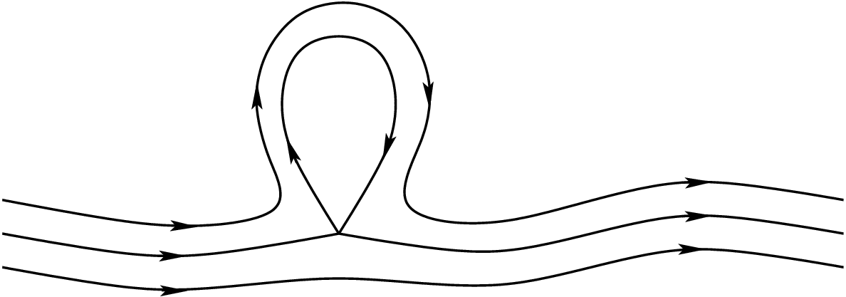
The non-singular closed trajectories in $\,{\bf p}$ - space are always locally stable and can be combined into connected cylinders consisting of trajectories of this type. In the case when a connected component of the Fermi surface does not consist of the closed trajectories only, these cylinders have finite heights and are bounded by singular closed trajectories (Fig. 14).

Let us make now the following reconstruction of the Fermi surface:

We remove all the cylinders of closed trajectories from the Fermi surface and fill the created holes by 2-dimensional discs orthogonal to $\,{\bf B}\,$ (Fig. 15).

It is easy to see that the reconstructed Fermi surface carries the same open electron trajectories as the initial one, so we can investigate the behavior of open trajectories on the reconstructed surface.

The reconstructed Fermi surface represents a 3-periodic surface which contains in general infinitely many connected components in $\,{\bf p}$ - space. One important theorem can be formulated about the connected components of the reconstructed Fermi surface in the case of presence of stable open trajectories ([36, 8, 10]):

Every connected component of the reconstructed Fermi surface carrying open electron trajectories represents a periodic deformation of an integral plane in $\,{\bf p}$ - space.

Let us remind here that the plane $\,\Gamma\,$ is called integral if it is generated by any two reciprocal lattice vectors. So, every connected component of the reconstructed Fermi surface has two independent periods represented by two vectors of the reciprocal lattice. Let us note also that the picture described above is evidently stable with respect to all small rotations of $\,{\bf B}\,$ view the local stability of nonsingular closed trajectories on the Fermi surface.

All the connected components of the reconstructed Fermi surface are parallel to each other which leads to the coinciding of the mean directions of all stable open trajectories in $\,{\bf p}$ - space. The last property was called in [25, 26] the Topological Resonance and plays very important role in the experimental observation of the anisotropic regimes of conductivity behavior and of the Topological Numbers corresponding to a given Stability Zone.

In this paper we will use the picture described above as the general picture arising in the case of presence of stable non-closed electron trajectories on the Fermi surface. Let us note here that this picture can have some additional features for some special directions of $\,{\bf B}\,$ within the Stability Zone (see [10]) which can be also detected from the experimental point of view ([25, 26]). These phenomena, however, have a non-generic character and will not be considered here.

After the factorization over the vectors of the reciprocal lattice every connected component of the reconstructed Fermi surface becomes a two-dimensional torus $\,\mathbb{T}^{2}\,$ embedded in $\,\mathbb{T}^{3}$. The number of non-equivalent components in $\,\mathbb{T}^{3}\,$ is always finite and represents an even number.

The open (in $\,{\bf p}$ - space) trajectories of system (I.1) on the Fermi level are given by the intersections of the components of the reconstructed Fermi surface with the planes orthogonal to $\,{\bf B}\,$ and represent irrational coverings of the corresponding tori $\,\mathbb{T}^{2}\,$ (except the discs $\,D^{2}$) in generic situation (Fig. 16 a). However, for special directions of $\,{\bf B}\,$ the intersection of the plane orthogonal to $\,{\bf B}\,$ with the integral plane $\,\Gamma_{\alpha}\,$ (${\bf B}\,\in\,\Omega_{\alpha}$) can have rational (integral) direction, which means in fact that the corresponding trajectories of (I.1) become periodic in $\,{\bf p}$ - space. The corresponding trajectories in $\,\mathbb{T}^{3}\,$ become now closed curves on the tori $\,\mathbb{T}^{2}\,$ and are not dense anymore on the sets $\,\mathbb{T}^{2}\,\setminus\cup\,D^{2}_{i}$ , which can be called the “carriers of open trajectories” on the Fermi surface (Fig. 16 b).

As we can see, the generic and the periodic open trajectories demonstrate an obvious difference in their statistical properties on the “carriers of open trajectories”. As will see below, this circumstance will play important role for the behavior of the conductivity tensor $\,\sigma^{kl}({\bf B})\,$ in the limit $\,\omega_{B}\tau\,\rightarrow\,\infty\,$.

We can see here that the periodic trajectories can not appear for completely irrational directions of $\,{\bf B}\,$ since the plane orthogonal to $\,{\bf B}\,$ should contain at least one vector of the reciprocal lattice, giving the mean direction of such trajectories. Let us note that the class of rationality of a direction of magnetic field $\,{\bf B}\,$ is defined as the number of linearly independent reciprocal lattice vectors lying in the plane orthogonal to $\,{\bf B}$. In particular, the direction $\,\hat{\bf B}^{0}_{\alpha}$, orthogonal to the plane $\Gamma_{\alpha}$, represents a purely rational direction according to this definition.

In general, it is not difficult to see that the directions of $\,{\bf B}\,$ in a Stability Zone $\,\Omega_{\alpha}$, corresponding to periodic open trajectories, form a dense net of one-dimensional curves, which do not intersect each other in $\,\Omega_{\alpha}\,$ in the case when the direction $\,\hat{\bf B}^{0}_{\alpha}\perp\Gamma_{\alpha}\,$ does not belong to $\,\Omega_{\alpha}\,$ (Fig. 9 a) or all intersect at the point $\,\hat{\bf B}^{0}_{\alpha}\,\,$ if $\,\,\hat{\bf B}^{0}_{\alpha}\in\Omega_{\alpha}\,$ (Fig. 9 b).

As we already said above, all the one-dimensional curves $\,\gamma^{\alpha}_{\bf a}\,$ should be actually extended outside the Stability Zone $\,\Omega_{\alpha}\,$ since the periodic open trajectories exist in fact for a wider set of directions of $\,{\bf B}\,$ surrounding $\,\Omega_{\alpha}$. The periodic open trajectories become unstable with respect to small rotations of $\,{\bf B}\,$ outside $\,\Omega_{\alpha}$. We have to note also that the difference between the curves $\,\gamma^{\alpha}_{\bf a}\,$ and $\,{\hat{\gamma}}^{\alpha}_{\bf a}\,$ decreases with increasing of the “denominator” of a rational mean direction of the periodic trajectories and vanishes in the limit $\,|{\bf a}|\,\rightarrow\,\infty\,$ (Fig. 10).

Let us consider now the carriers of open trajectories in more detail.

The general form of connected components of the reconstructed Fermi surface is shown at Fig. 17 and represents a periodically deformed integral plane in $\,{\bf p}$ - space with two periods $\,{\bf q}_{1}$, $\,{\bf q}_{2}$,   given by two independent reciprocal lattice vectors.

The carriers of open trajectories in $\,{\bf p}$ - space represent the same periodically deformed integral planes without “artificial” two-dimensional discs $\,D^{2}$, attached after the removal of closed trajectories. Let us exclude here the non-generic case when the magnetic field $\,{\bf B}\,$ is orthogonal to the plane $\,\Gamma_{\alpha}\,$ and consider the generic case

We will assume in our considerations that the $z$ - axis is always chosen along the direction of $\,{\bf B}\,$ while the $x$ -   and $y$ - axis are orthogonal to $\,{\bf B}$. In the generic situation described above the values of $\,p_{z}\,$ separate all different trajectories at a given component and $\,p_{z}\,$ can be chosen as a “coordinate” on the corresponding carrier of open trajectories.

The second coordinate on the carriers of open trajectories is naturally given by the parameter $\,t$, measured along the trajectories according to system (I.1).

In general, a natural system of local coordinates in $\,{\bf p}$ - space (or $\,\mathbb{T}^{3}$) is given by the triple $\,(p_{z},\,t,\,\epsilon)\,$ if we consider system (I.1) for all values of $\,\epsilon\,$. The coordinates $\,(p_{z},\,t,\,\epsilon)\,$ are naturally connected with system (I.1) and possess also one more remarkable property:

References

- [1] A.A. Abrikosov., Fundamentals of the Theory of Metals., Elsevier Science & Technology, Oxford, United Kingdom, 1988.
- [2] V.I. Arnol’d., Topological and ergodic properties of closed 1-forms with incommensurable periods., Functional Analysis and Its Appl. 25:2 (1991), 81-90.
- [3] R. De Leo., Existence and measure of ergodic leaves in Novikov’s problem on the semiclassical motion of an electron., Russian Math. Surveys 55:1 (2000), 166-168.
- [4] R. De Leo., Characterization of the set of “ergodic directions” in Novikov’s problem of quasi-electron orbits in normal metals., Russian Math. Surveys 58:5 (2003), 1042-1043.
- [5] R. De Leo., Topology of plane sections of periodic polyhedra with an application to the Truncated Octahedron., Experimental Mathematics 15:1 (2006), 109-124.
- [6] R. De Leo, I.A. Dynnikov., An example of a fractal set of plane directions having chaotic intersections with a fixed 3-periodic surface., Russian Math. Surveys 62:5 (2007), 990–992.
- [7] R. De Leo, I.A. Dynnikov., Geometry of plane sections of the infinite regular skew polyhedron ., Geom. Dedicata 138:1 (2009), 51-67.
- [8] I.A. Dynnikov., Proof S.P. Novikov’s conjecture on the semiclassical motion of an electron., Math. Notes 53:5 (1993), 495-501.
- [9] I.A. Dynnikov., Semiclassical motion of the electron. A proof of the Novikov conjecture in general position and counterexamples., Solitons, geometry, and topology: on the crossroad, Amer. Math. Soc. Transl. Ser. 2, 179, Amer. Math. Soc., Providence, RI, 1997, 45-73.
- [10] I.A. Dynnikov., The geometry of stability regions in Novikov’s problem on the semiclassical motion of an electron., Russian Math. Surveys 54:1 (1999), 21-59.
- [11] I.A. Dynnikov., Interval Identification Systems and Plane Sections of 3-Periodic Surfaces., Proc. Steklov Inst. Math. 263 (2008), 65-77.
- [12] I. Dynnikov, A. Skripchenko., On typical leaves of a measured foliated 2-complex of thin type., Topology, Geometry, Integrable Systems, and Mathematical Physics: Novikov’s Seminar 2012-2014, Advances in the Mathematical Sciences., Amer. Math. Soc. Transl. Ser. 2, 234, eds. V.M. Buchstaber, B.A. Dubrovin, I.M. Krichever, Amer. Math. Soc., Providence, RI, 2014, 173-200, arXiv: 1309.4884
- [13] R.N. Gurzhy, A.I Kopeliovich., Low-temperature electric conductivity of pure metals., In the book: Conductivity electrons., Red. M.I. Kaganov, V.S. Edelman., Moscow, Nauka, 1985 (in Russian).
- [14] A.Ya. Hinchin, Continued fractions., Moscow: FISMATGIS, (1961).
- [15] M.I. Kaganov, V.G. Peschansky., Galvano-magnetic phenomena today and forty years ago., Physics Reports 372 (2002), 445-487.
- [16] C. Kittel., Quantum Theory of Solids., Wiley, 1963.
- [17] I.M.Lifshitz, M.Ya.Azbel, M.I.Kaganov. Sov. Phys. JETP 4 (1957), 41.
- [18] I.M. Lifshitz, V.G. Peschansky., Galvanomagnetic characteristics of metals with open Fermi surfaces., Sov. Phys. JETP 8 (1959), 875.
- [19] I.M. Lifshitz, V.G. Peschansky., Galvanomagnetic characteristics of metals with open Fermi surfaces. II., Sov. Phys. JETP 11 (1960), 137.
- [20] I.M. Lifshitz, M.I. Kaganov., Some problems of the electron theory of metals I. Classical and quantum mechanics of electrons in metals., Sov. Phys. Usp. 2:6 (1960), 831-835.
- [21] I.M. Lifshitz, M.I. Kaganov., Some problems of the electron theory of metals II. Statistical mechanics and thermodynamics of electrons in metals., Sov. Phys. Usp. 5:6 (1963), 878-907.
- [22] I.M. Lifshitz, M.I. Kaganov., Some problems of the electron theory of metals III. Kinetic properties of electrons in metals., Sov. Phys. Usp. 8:6 (1966), 805-851.
- [23] I.M. Lifshitz, M.Ya. Azbel, M.I. Kaganov., Electron Theory of Metals. Moscow, Nauka, 1971. Translated: New York: Consultants Bureau, 1973.
- [24] A.Y. Maltsev., Anomalous behavior of the electrical conductivity tensor in strong magnetic fields., JETP 85 (5) (1997), 934-942.
- [25] A.Ya. Maltsev, S.P. Novikov., Quasiperiodic functions and Dynamical Systems in Quantum Solid State Physics., Bulletin of Braz. Math. Society, New Series 34:1 (2003), 171-210.
- [26] A.Ya. Maltsev, S.P. Novikov., Dynamical Systems, Topology and Conductivity in Normal Metals in strong magnetic fields., Journal of Statistical Physics 115:(1-2) (2004), 31-46.
- [27] S.P. Novikov., The Hamiltonian formalism and a many-valued analogue of Morse theory., Russian Math. Surveys 37 (5) (1982), 1-56.
- [28] S.P. Novikov, A.Y. Maltsev., Topological quantum characteristics observed in the investigation of the conductivity in normal metals., JETP Letters 63 (10) (1996), 855-860.
- [29] S.P. Novikov, A.Y. Maltsev., Topological phenomena in normal metals., Physics-Uspekhi 41:3 (1998), 231-239.
- [30] T. Osada, S. Kagoshima, N. Miura., Resonance effect in magnetotransport anisotropy of quasi-one-dimensional conductors., Phys. Rev. B 46:3 (1992-I), 1812.
- [31] Ya.G. Sinai, K.M. Khanin., Mixing for some classes of special flows over rotations of the circle., Functional Analysis and Its Appl. 26:3 (1992), 155-169.
- [32] A. Skripchenko., Symmetric interval identification systems of order three., Discrete Contin. Dyn. Sys. 32:2 (2012), 643-656.
- [33] A. Skripchenko., On connectedness of chaotic sections of some 3-periodic surfaces., Ann. Glob. Anal. Geom. 43 (2013), 253-271.
- [34] S.P. Tsarev. Private communication. (1992-93).
- [35] J.M. Ziman., Principles of the Theory of Solids., Cambridge Univ. Press 1972.
- [36] A.V. Zorich., Russian Math. Surveys 39, 287 (1984).
- [37] A.V. Zorich., Proc. “Geometric Study of Foliations”., (Tokyo, November 1993) / ed. T.Mizutani et al. Singapore: World Scientific, 479-498 (1994).