Effective Capacity in MIMO Channels with Arbitrary Inputs

Following the research of Foschini [1] and Telatar [2], multiple-input and multiple-output (MIMO) transmission systems have been widely studied, and it was shown that employing multiple antennas at a transmitter and/or a receiver can remarkably enhance the system performance in terms of both reliability and spectral efficiency [3]. Herein, the information-theoretic analysis of MIMO systems formed the basis to understand the system dynamics [4, 5, 6, 7, 8, 9, 10, 11, 12, 13, 14]. For instance, the ergodic capacity of MIMO systems was explored, and analytical characterizations of spatial fading correlations and their effect on the ergodic capacity were provided in [5]. Moreover, regarding the available information about the channel statistics at the transmitter, the optimal input covariance matrix that achieves the maximum ergodic capacity in a one-to-one MIMO system was investigated in [6]. Considering line-of-sight characterizations in a wireless medium, the structures of the capacity-achieving input covariance matrices were researched as well [12, 13, 14].

The efficient use of energy is a fundamental requirement in communication networks because most of the portable communication devices are battery-driven and environmental concerns are to be carefully mediated. Thus, energy efficiency along with spectral efficiency is in the focus of attention in prospective transmission system designs. For example, the next generation wireless communication technology, commonly known as 5G, targets to support 10 to 100 times higher data transmission rate and to provide 10 times longer battery life than the preceding mobile technology [15]. In this regard, the ergodic capacity of MIMO systems were primarily studied in low-power regimes [16, 17, 18, 19]. These studies revealed that when the objective capacity function is concave, the minimum energy required to transmit one bit of information, i.e., energy-per-bit, is obtained when the signal-to-noise ratio approaches zero [16]. Subsequently, a more comprehensive energy efficiency analysis was conducted considering any power regime [20]. Particularly, MIMO scenarios with Rayleigh fading channel models were investigated, and a fairly accurate closed-form approximation for the energy-per-bit was obtained by engaging different power models. Similar investigations were conducted in distributed MIMO systems as well [21].

Another approach that maximizes the spectral efficiency while minimizing the energy-per-bit is to increase the spatial dimension by increasing the number of transmit and/or receive antennas. It was shown that the spectral efficiency improves substantially with the increasing number of antennas while making the transmit power arbitrarily small [22]. On this account, massive MIMO (or large-scale antenna [23]) systems have evolved as a candidate technology for 5G wireless communications [24, 25], and they have been investigated from information-theoretic perspectives [26, 27, 28, 29, 30, 31, 32]. Particularly, energy and spectral efficiency in the uplink channels of multi-user massive MIMO systems were studied with different information processing techniques such as maximum-ratio combining, zero forcing, and minimum mean-square error (MMSE) estimation [29]. Likewise, power allocation policies were also studied and optimal input covariance matrices in multi-access channels with massive number of antennas at both transmitters and receivers, which maximize the sum transmission rate, were derived [32].

Quality-of-service (QoS) constraints, which generally emerge in the form of delay and/or data buffering limitations, are generally disregarded when the ergodic capacity is set as the only performance metric. However, the increasing demand for delay-sensitive services, such as video streaming and online gaming over wireless networks, has brought up the need for a comprehensive investigation of delay-sensitive scenarios [33]. For wireless communications systems with such delay-sensitive services, the ergodic capacity solely is not a sufficient metric. On the contrary, QoS constraints in the data-link layer that are attributed to delay violation and buffer overflow probabilities should be invoked as performance measures as well. Relying on this motivation, cross-layer design goals were acquired as new research grounds. Initial cross-layer analysis was performed in wired networks, where the effective bandwidth (the minimum required service rate from a transmission node given a data arrival process at that node under desired QoS requirements) was introduced as a performance probing tool [34, 35]. In effective bandwidth studies, stochastic nature of data arrival processes were taken into account while assuming service processes with constant transmission rates. However, in contrast to the deterministic nature of wired networks, wireless service links demonstrate generally a stochastic behavior, and the instantaneous transmission (service) rates may vary drastically. In this context, the effective capacity, which provides the maximum constant data arrival rate at a transmission node that is sustained by a given stochastic service process under defined QoS constraints, was proposed [36]. The effective capacity is the dual of the effective bandwidth. The concept of the effective capacity has gained a notable attention, and it has been investigated in several transmission scenarios, including MIMO systems [37, 38, 39]. Specifically, point-to-point MIMO scenarios were explored under QoS constraints by employing the effective capacity as the performance metric in the low and high signal-to-noise ratio regimes and the wide-band regime [37]. A comparable analysis was extended to cognitive MIMO systems, where the effects of channel uncertainty on the effective capacity performance of secondary users following channel sensing errors are studied [38]. Regarding the antenna beam-forming, optimal transmit strategies that maximize the effective capacity were derived in MIMO systems with doubly correlated channels and a covariance feedback [39].

Because Gaussian input signaling in certain cases is optimal in the sense of maximizing the mutual information between the input and output in a transmission channel, it has been invoked in many research scenarios. Even though Gaussian input signaling is not practical, it is preferred by many researchers since it typically simplifies the analytical presentations. On the other hand, it is of importance to understand the effects of signaling choice on the the system performance, because the type of input signaling may critically affect the tradeoff between the data arrival process to a node and the data service process from that node [40]. A general look at wireless systems employing finite and discrete input signaling methods can be found in [41, 42, 43, 44, 45, 46, 47, 48]. However, QoS constraints are generally not included in these studies. Particularly, the optimal precoding matrix in a point-to-point MIMO system, which maximizes the mutual information in the low and high signal-to-noise ratio regimes, was proposed [41]. With the same objective, channel diagonalization was applied in order to obtain the optimal channel precoder [43, 45], i.e., parallel and non-interfering Gaussian channels are formed to reach the optimal input covariance matrix. In another study [49], the optimal power allocation policy that maximizes the mutual information, named as mercury/water-filling, was shown to be a generalization to the well-known water-filling algorithm. Multi-access systems were studied as well [47], where linear precoding matrices are obtained in order to maximize the weighted sum rate. An extension of the same analysis was performed in scenarios in which transmitters have only statistical information about the wireless channels [48]. Asymptotic analyses in the large-scale antenna regimes were also provided. Here, the notion of mutual information was utilized as the performance metric, and the rudimentary relation between the mutual information and the MMSE, which was introduced in [50, 51], was exploited.

In this paper, we focus on a more general MIMO scenario in which input signaling is arbitrary and statistical QoS constraints. We investigate the system performance by employing the effective capacity. We provide a mathematical toolbox¹¹ 1 We refer interested readers to [52, 53, 54, 55] and references therein for practical massive MIMO settings. that system designers can use in order to understand performance levels of spectrum and energy efficient systems under QoS constraints imposed as limits on the buffer overflow and delay violation probabilities, which are two of the main objectives in the 5G technology [15]. More specifically, we can list our contributions as follows:

1. 1.

   Assuming that the instantaneous channel fading gain estimate is available at both the transmitter and the receiver, we have identified the optimal input covariance matrix that maximizes the effective capacity under a short-term average power constraint over the transmit antennas.

2. 2.

   We obtain the first and second derivatives of the effective capacity when the signal-to-noise ratio goes to zero. Using these derivatives, we obtain a linear approximation of the effective capacity in the low signal-to-noise ratio regime. We show that this approximation does not depend on the input distribution and covariance matrix.

3. 3.

   We further show that the minimum energy-per-bit is obtained when the signal-to-noise ratio goes to zero and that it is independent of the QoS constraints, the input distribution, and the covariance matrix.

4. 4.

   In the large-scale antenna regime, we prove that the effective capacity approaches the average mutual information in the channel, i.e., the dependence of the effective capacity performance on the QoS constraints decreases with the increasing number of antennas.

5. 5.

   Under the stability condition of the data queue, we analyze the non-asymptotic backlog and delay violation bounds by utilizing the effective capacity.

We can apply the analysis provided in the paper in different practical scenarios that necessitate low latency, low power consumption or ability to simultaneously support massive number of users. Here, we refer to the vehicular-based communication scenarios defined by the well-known European project ‘Mobile and wireless communications Enablers for the Twenty-twenty Information Society (METIS)’ [15, 56]. For instance, we can perform our analysis in scenarios such as ‘Best experience follows you’ [15] and ‘Traffic Jam’ and ‘Traffic Efficiency and Safety’ [56].

The rest of the paper is organized as follows: We describe the MIMO system in Section II. Then, we discuss the instantaneous mutual information between the channel input and output, and then introduce the effective rate and capacity expressions in Section III. We provide the optimal input covariance matrix. We perform asymptotic analyses in the low signal-to-noise ratio regime in Section IV-A and in the large-scale antenna regime in Section IV-B. We investigate non-asymptotic backlog and delay bounds in Section V. We present the numerical results in Section VI and the conclusion in Section VII. We relegate the proofs to the Appendix.

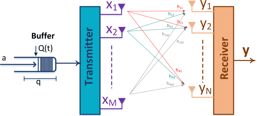
As shown in Figure 1, we consider a point-to-point MIMO transmission system in which one transmitter and one receiver are equipped with $M$ and $N$ antennas, respectively. The data generated by a source (or sources) initially arrives at the transmitter buffer with rate a(t) bits/channel use²² 2 Each channel use duration can be considered equal to the sampling duration of one symbol, i.e., bits/sec/Hz. for $t\in\{1,2,\cdots\}$ and is stored in the buffer. Following the encoding and modulation processes, the transmitter sends the data to the receiver over the wireless channel packet by packet in frames (blocks) of $T$ channel uses. During the transmission of the data, the input-output relation in the flat-fading channel at time instant $t$ is expressed as follows:

where $\boldsymbol{\mathrm{x}}_{t}$ and $\boldsymbol{\mathrm{y}}_{t}$ are the $M$-dimensional input and $N$-dimensional output vectors, respectively, and $\boldsymbol{\mathrm{w}}_{t}$ represents the $N$-dimensional additive noise vector with independent and identically distributed elements. Each element of $\boldsymbol{\mathrm{w}}_{t}$ is circularly symmetric, complex Gaussian distributed with zero-mean and variance $\sigma_{w}^{2}$. Hence, we have $\mathbb{E}\{\boldsymbol{\mathrm{w}}_{t}\boldsymbol{\mathrm{w}}_{t}^{\dagger}\}=\sigma_{w}^{2}\boldsymbol{\mathrm{I}}_{N\times N}$, where $\mathbb{E}\{\cdot\}$ denotes the expected value, $\{\cdot\}^{\dagger}$ is the transpose operator and $\boldsymbol{\mathrm{I}}_{N\times N}$ is the $N\times N$ identity matrix. Furthermore, $\mathbf{H}_{t}=\{h_{nm}(t)\}$ is the $N\times M$ random channel matrix, where $h_{nm}(t)$ is the channel fading coefficient with an arbitrary distribution between the $m^{\text{th}}$ transmit antenna and the $n^{\text{th}}$ receive antenna. Here, we consider a general channel model and assume that the distributions of $\{h_{nm}(t)\}$ can be either statistically identical or non identical or semi identical³³ 3 In semi-identical channel models, the channel coefficients from different transmit antennas to a common receive antenna at a receiver with multiple antennas are identically distributed, but the coefficients related to different receive antennas are non-identically distributed. Such a model fits into an uplink scenario of a cellular system, e.g., from a handset to a base station, where the antennas on the handset are installed in a small panel and the antennas at the base station are mounted several wavelengths apart from each other [57].. We further assume that the channel matrix remains constant during one transmission frame ($T$ channel uses) and changes independently from one frame to another. We also consider a short-term power constraint, i.e., $P$ indicates the power allocated for the transmission of the data in one channel use. Then, we have $\mathbf{tr}\{\mathbb{E}\{\boldsymbol{\mathrm{x}}_{t}\boldsymbol{\mathrm{x}}_{t}^{\dagger}\}\}=\mathbf{tr}\{\boldsymbol{\mathrm{K}}_{t}\}\leq 1$, where $\mathbf{tr}\{\cdot\}$ is the trace operator and $\boldsymbol{\mathrm{K}}_{t}$ is a positive semi-definite Hermitian matrix.

We assume that the instantaneous channel realizations are available at both the transmitter and the receiver, and that the channel fading coefficients are correlated with each other. We invoke the Kronecker product model, which is widely used in modeling real channels because of its analytical tractability with a reasonable accuracy [58, Ch. 2], [59]. Hence, the channel matrix is expressed as

where $\Gamma_{t}$ is an $N\times M$ matrix with independent and identically distributed complex elements. $\mathbf{R}_{v}$ and $\mathbf{R}_{r}$ are the transmit and receive correlation matrices, respectively, which are usually modeled with an exponential correlation structure [60, 61]. The transmit and receive correlation matrices depend on the array spacing at the transmitter and the receiver, and the characteristic distances proportional to the spatial coherence distances at the transmitter and the receiver, respectively. Particularly, the elements of $\mathbf{R}_{v}$ and $\mathbf{R}_{r}$ are expressed as $\{\mathbf{R}_{v}\}_{kl}=e^{\frac{d_{v}}{\Delta_{v}}|k-l|}$ for $\quad k,l\in\{1,\cdots,M\}$ and $\{\mathbf{R}_{r}\}_{kl}=e^{\frac{d_{r}}{\Delta_{r}}|k-l|}$ for $\quad k,l\in\{1,\cdots,N\}$, respectively, where $d_{v}$ and $d_{r}$ are the corresponding antenna spacings, and $\Delta_{v}$ and $\Delta_{r}$ are the corresponding characteristic distances. Therefore, the correlation matrix at one end can be locally estimated without any feedback from the other end. On the other hand, $\Gamma_{t}$ is estimated by the receiver, and then forwarded to the transmitter at the beginning of each transmission frame⁴⁴ 4 Similar to the strategy in [62, 63, 64], we assume that the feedback channel is delay-free and error-free. Because we have a block-fading channel, the channel information is valid until the end of the transmission frame. Even if we consider a feedback delay, it will only reduce the time allocated for data transmission. In particular, when the channel feedback arrives after a certain portion of the time frame ($T$ channel uses), i.e., $\alpha T$ for $0<\alpha<1$, the remaining $(1-\alpha)T$ will be the time duration for data transmission. Moreover, the reliable feedback can be sustained with strong channel codes.. We further know that in practical settings the channel estimation is obtained imperfectly. Therefore, we have

where $\widehat{\Gamma}_{t}$ is the channel estimate and $\widetilde{\Gamma}_{t}$ is the channel estimation error. Given that the receiver employs MMSE estimator in order to obtain the channel knowledge, we have $\widehat{\Gamma}_{t}$ and $\widetilde{\Gamma}_{t}$ uncorrelated with each other. Similar to [64], we further assume that $\widetilde{\Gamma}_{t}$ is a zero-mean process with a known variance at both the transmitter and the receiver. Above, $\widehat{\mathbf{H}}_{t}=\mathbf{R}_{r}^{\frac{1}{2}}\widehat{\Gamma}_{t}\mathbf{R}_{v}^{\frac{1}{2}}$ and $\widetilde{\mathbf{H}}_{t}=\mathbf{R}_{r}^{\frac{1}{2}}\widetilde{\Gamma}_{t}\mathbf{R}_{v}^{\frac{1}{2}}$. Hence, the input-output relation in (1) becomes

Due to the time-varying nature of wireless channels, it is not very easy to sustain a stable transmission rate. In particular, reliable transmission may not be provided all the time. Therefore, depending on the type of data transmission, delay violation and buffer overflow concerns become critical at the transmitter. Respectively, given a statistical transmission (service) process, how to determine the maximum data arrival rate at the transmitter buffer so that the QoS requirements in the form of limits on delay violation and buffer overflow probabilities can be satisfied is one of the main research questions. In this regard, the effective capacity can be employed as a performance metric. Specifically, the effective capacity identifies the maximum constant data arrival rate at the transmitter buffer that the time-varying transmission process can support under desired QoS constraints [36].

In Fig. 1, $Q(t)$ is the number of bits in the data buffer at time instant $t$ and $q$ is the buffer threshold. Now, let $Q=Q(t\to\infty)$ be the steady-state queue length and $\theta$ be the decay rate of the tail distribution of the queue length, $Q$. Then, $\theta$ is defined as [34, Theorem 3.9]

$\theta$ is also called as the QoS exponent. Now, we can easily approximate the buffer overflow probability⁵⁵ 5 The constraint on the overflow probability can be linked to the constraint on the queuing delay probability. For instance, it has been shown that $\Pr\{D\geq d_{\max}\}\leq c\sqrt{\Pr\{Q\geq q_{\max}\}}$ for constant arrival rates, where $D$ is the steady-state delay experienced at the buffer, $c$ is a constant, and $q_{\max}=ad_{\max}$, where $a$ is the data arrival rate [65]. as $\text{Pr}(Q\geq q_{\max})\approx e^{-\theta q_{\max}}$ for a large threshold, $q_{\max}$. Here, larger $\theta$ implies stricter QoS constraints, whereas smaller $\theta$ corresponds to looser constraints. Subsequently, for a given discrete-time, ergodic and stationary stochastic service process, $r(t)$, the effective capacity as a function of the decay rate parameter, $\theta$, is given by [36, Eq. (11)]

where $r(t)$ is the service rate in the wireless channel at time instant $t$, $\sum_{t=1}^{\tau T}r(t)$ is the time-accumulated service process, i.e., the total number of bits served from the transmitter in $\tau T$ channel uses, and $\tau\in\{1,2,\cdots,\}$ is the time frame index. Recall that the encoding and modulation of data and its transmission are performed in frames of $T$ channel uses.

Given the channel estimate, $\widehat{\mathbf{H}}_{t}$, the service rate in one frame can be set to the mutual information between $\mathbf{x}_{t}$ and $\mathbf{y}_{t}$, i.e., $r(t)=\mathcal{I}(\mathbf{x}_{t};\mathbf{y}_{t}|\widehat{\mathbf{H}}_{t})$. However, considering the input-output relation (4), it is difficult to evaluate the mutual information in closed-form. Therefore, the service rate in the channel is set to a lower bound on the mutual information by considering the worst-case noise and modeling the estimation error as an additional Gaussian noise vector with zero-mean, independent and identically distributed samples [66, 67], i.e., $r(t)=\mathcal{I}_{L}(\mathbf{x}_{t};\mathbf{y}_{t}|\widehat{\mathbf{H}}_{t})\leq\mathcal{I}(\mathbf{x}_{t};\mathbf{y}_{t}|\widehat{\mathbf{H}}_{t})$ and $\mathbb{E}\{\widetilde{\mathbf{w}}_{t}\widetilde{\mathbf{w}}_{t}^{\dagger}\}=\sigma_{\widetilde{w}}^{2}\mathbf{I}_{N\times N}$, where $\sigma_{\widetilde{w}}^{2}=\sigma_{w}^{2}+\frac{P}{NM}\mathbf{tr}\left\{\mathbb{E}\left\{\widetilde{\mathbf{H}}_{t}\mathbf{x}_{t}\mathbf{x}_{t}^{\dagger}\widetilde{\mathbf{H}}_{t}^{\dagger}\right\}\right\}$. Since the service rate in the channel is smaller than or equal to the mutual information, the reliable transmission is guaranteed. Hence, the service rate is expressed as

where $f_{\boldsymbol{\mathrm{y}}_{t}}(\boldsymbol{\mathrm{y}}_{t})=\sum_{\boldsymbol{\mathrm{x}}_{t}}p(\boldsymbol{\mathrm{x}}_{t})f_{\boldsymbol{\mathrm{y}}_{t}|\boldsymbol{\mathrm{x}}_{t}}(\boldsymbol{\mathrm{y}}_{t}|\boldsymbol{\mathrm{x}}_{t})$ is the probability density function of $\boldsymbol{\mathrm{y}}_{t}$ and $f_{\boldsymbol{\mathrm{y}}_{t}|\boldsymbol{\mathrm{x}}_{t}}(\boldsymbol{\mathrm{y}}_{t}|\boldsymbol{\mathrm{x}}_{t})=(\pi\sigma_{\widetilde{w}}^{2})^{-N}e^{-\frac{1}{\sigma_{\widetilde{w}}^{2}}||\boldsymbol{\mathrm{y}}_{t}-\sqrt{P}\,\widehat{\mathbf{H}}_{t}\,\boldsymbol{\mathrm{x}}_{t}||^{2}}$ is the conditional probability density function of $\boldsymbol{\mathrm{y}}_{t}$ given $\boldsymbol{\mathrm{x}}_{t}$. For notational convenience in the paper, we use $\mathcal{I}(\mathbf{x}_{t};\mathbf{y}_{t})$ to refer to the lower bound, $\mathcal{I}_{L}(\mathbf{x}_{t};\mathbf{y}_{t}|\widehat{\mathbf{H}}_{t})$.

Because the channel matrix stays constant during one transmission frame and changes independently⁶⁶ 6 As for the effective capacity when there exists a temporal correlation between the channel matrices, we refer to [35, Chap. 7, Example 7.2.7]. Because we focus on the performance levels in the low signal-to-noise ratio and large-scale antenna regimes, we consider a temporally uncorrelated channel model. from one frame to another, and that the encoding and modulation of the data packets are performed in $T$ channel uses, we can express the normalized effective rate in bits/channel use/receive dimension as

Above, while the receiver has the instantaneous channel estimate, the transmitter has no information regarding the channel matrix. If the transmitter is aware of the channel statistics but not the actual value of $\widehat{\mathbf{H}}_{t}$, then the transmitter sets the input covariance matrix to a value, i.e., $\boldsymbol{\mathrm{K}}_{t}=\boldsymbol{\mathrm{K}}$, in order to maximize the effective rate in (7) by considering the QoS constraints and the channel statistics, i.e.,

in bits/channel use/receive dimension. In (8), the covariance matrix, $\boldsymbol{\mathrm{K}}$, depends on the statistics of $\widehat{\mathbf{H}}_{t}$ and the worst-case noise, and is independent of its actual realization. On the other hand, if the instantaneous knowledge of $\widehat{\mathbf{H}}_{t}$ is available at the transmitter and the receiver, the transmitter can adaptively set the input covariance matrix by considering both the QoS constraints and the instantaneous realization of the channel matrix⁷⁷ 7 In case there is a delay in the feedback channel, and the delay is smaller than the block duration ($T$ channel uses), the effective capacity can be reformulated as $C_{E}(\theta)=-\frac{1}{\theta NT}\log_{\text{e}}\mathbb{E}_{\widehat{\mathbf{H}}_{t}}\left\{e^{-\theta T(1-\alpha)\mathcal{I}(\boldsymbol{\mathrm{x}}_{t};\boldsymbol{\mathrm{y}}_{t})}\right\}$, where $\alpha T$ is the delay and $0<\alpha<1$.. Hence, the maximum effective rate, which we call as the effective capacity, in bits/channel use/receive dimension is given as follows:

Above, $\boldsymbol{\mathrm{K}}_{t}$ is time-varying unlike $\boldsymbol{\mathrm{K}}$ in (8), because it is a function of $\widehat{\mathbf{H}}_{t}$.

Here, a key research problem is the optimal selection of the power allocation policy (or input covariance matrix) given the channel matrix and the QoS requirements. In particular, the central question is the following: What is the instantaneous input covariance matrix, $\boldsymbol{\mathrm{K}}_{t}$, that solves (9) given that the channel matrix, $\widehat{\mathbf{H}}_{t}$, is available at the transmitter and the receiver, and that there are certain QoS constraints? In the following theorem, we identify the optimal policy that the transmitter should employ to obtain (9).

Proof: See Appendix -A.$\hfill{\square}$

In (10), both the mutual information and $\mathbf{mmse}_{t}$ are functions of the input covariance matrix, $\boldsymbol{\mathrm{K}}_{t}$, and (10) is non-concave over the space spanned by $\boldsymbol{\mathrm{K}}_{t}$ [44, 42, 45]. Therefore, the solution obtained from (10) is not necessarily unique. On the other hand, we follow a different strategy and start with the singular value decomposition of the channel matrix, i.e.,

where $\boldsymbol{\mathrm{U}}_{t}$ and $\boldsymbol{\mathrm{V}}_{t}$ are $N\times N$ and $M\times M$ unitary matrices, respectively, and $\boldsymbol{\mathrm{D}}_{t}$ is an $N\times M$ matrix with non-negative real numbers on the diagonal, which are the square roots of the non-zero eigenvalues of $\widehat{\mathbf{H}}_{t}\widehat{\mathbf{H}}_{t}^{\dagger}$ and $\widehat{\mathbf{H}}_{t}^{\dagger}\widehat{\mathbf{H}}_{t}$. Then, we re-express the input-output model in (4) as follows:

where $\widetilde{\boldsymbol{\mathrm{y}}}_{t}=\boldsymbol{\mathrm{U}}_{t}^{\dagger}\boldsymbol{\mathrm{y}}_{t}$ and $\widetilde{\boldsymbol{\mathrm{x}}}_{t}=\boldsymbol{\mathrm{V}}_{t}^{\dagger}\boldsymbol{\mathrm{x}}_{t}$. The new noise vector is denoted by $\widetilde{\boldsymbol{\mathrm{n}}}_{t}=\boldsymbol{\mathrm{U}}_{t}^{\dagger}\widetilde{\mathbf{w}}_{t}$, which is a zero-mean, Gaussian, complex vector with independent and identically distributed elements [2]. We further know that $\mathcal{I}(\boldsymbol{\mathrm{x}}_{t};\boldsymbol{\mathrm{y}}_{t})=\mathcal{I}(\widetilde{\boldsymbol{\mathrm{x}}}_{t};\widetilde{\boldsymbol{\mathrm{y}}}_{t})$, because the information regarding $\widehat{\mathbf{H}}_{t}$ is available at both the transmitter and the receiver. Now, let $\widetilde{\boldsymbol{\mathrm{K}}}_{t}$ be the covariance matrix of $\widetilde{\boldsymbol{\mathrm{x}}}_{t}$ , i.e.,

In particular, if we can find the optimal $\widetilde{\boldsymbol{\mathrm{K}}}_{t}$, we can also determine the optimal input covariance matrix, $\boldsymbol{\mathrm{K}}_{t}$. Therefore, we provide the optimal input covariance matrix in the following theorem and show that this is the global solution in its proof.

Proof: See Appendix -B.$\hfill{\square}$

Having obtained the effective capacity and rate expressions, and having characterized the optimal input covariance matrices that maximize the effective capacity performance, we note that due to the complexity in the analytical formulations, it becomes difficult to gain insight on the system performance in general scenarios. On the other hand, asymptotic approaches can help us set the design criteria in certain asymptotic regimes. Therefore, we investigate the effective capacity of MIMO systems in the low signal-to-noise ratio and large-scale antenna regimes. We also note that we drop the time index in the sequel unless otherwise it becomes necessary.

So far, we have investigated the throughput and energy efficiency of the aforementioned MIMO systems in two different asymptotic regimes by employing the effective capacity, which is also an asymptotic measure in time. Nevertheless, non-asymptotic performance bounds regarding the statistical characterizations of buffer overflow and queueing delay are of importance for practical research agendas. Therefore, we benefit from the tools of the stochastic network calculus [71, 72, 73], and provide a statistical bound on the buffer overflow and queueing delay probabilities by utilizing the effective capacity.

Recall that the transmission of a packet is performed over a block duration of $T$ channel uses and the transmission rate in the channel during one transmission block is constant. Now, let us define $s(i)$ as the total number of bits transmitted (served) in the $i^{\text{th}}$ transmission block. Subsequently, considering the normalized effective rate for the input covariance matrix given in (7), $R_{E}(\theta)$, and following the setting in [73, Definition 7.2.1], we define a statistical affine bound for the aforementioned channel model for any decay rate value, $\theta$, as follows:

where $S(i,j)=\sum_{l=i+1}^{j}s(l)$, and $\sigma_{R}(\theta)$ is a slack term that defines an initial transmission delay. Due to $-\theta$, the expression in (29) is in fact a lower bound on the expected amount of the transmitted data in the channel. Subsequently, noting Chernoff’s lower bound $\Pr\{X\leq x\}\leq e^{\theta x}\mathbb{E}\{e^{-\theta X}\}$ for $\theta\geq 0$, we have the exponentially bounded fluctuation model described in [74] with parameters $R_{E}(\theta)>0$ and $b\geq 0$ as

where $\varepsilon(b)=e^{\theta\sigma_{R}(\theta)}e^{-\theta b}$ is a specific exponentially decaying deficit profile of the amount of the transmitted data in the channel. Now, using the union bound, we express the sample path guarantee as follows:

where

and $NTR^{\star}_{E}(\theta)=NTR_{E}(\theta)-\delta$ with a free parameter $0<\delta\leq NTR_{E}(\theta)-Ta$ for a constant data arrival rate at the transmitter buffer, i.e., $a$ bits/channel use. For a more detailed derivation, we refer to [73]. We also refer to [75], where capacity-delay-error boundaries are provisioned as performance models for networked sources and systems. Exclusively, the backlog at the transmitter buffer with the constant data arrival rate $a$, i.e.,

has a statistical bound

and may fail with probability $\Pr\{Q(j)>q\}\leq\varepsilon^{{}^{\prime}}(b)$, where $[x]_{+}=0$ if $x<0$ and $[x]_{+}=x$ otherwise, which accounts for $S(i,j)\geq 0$. In this place, if $a\leq NR_{E}^{\star}(\theta)$ for stability,

is valid for all $j$. Accordingly, we can express the delay bound $\Pr\{D(j)>d\}$ with $d=\frac{q}{a}$, which is expressed in channel use. In other words, $\frac{Tb}{NTR_{E}(\theta)-\delta}$ in (31) provides us the initial latency caused by the variations in the transmission. Finally, we can express $b$ by inversion of (30) for any given $\varepsilon^{{}^{\prime}}$ as

As for the existence of the slack term in (32), we refer to the following Lemma.

In this section, we substantiate our analytical results through numerical analysis. We initially assume that the channel is perfectly known at both the transmitter and receiver, and that the channel coefficients are uncorrelated, i.e., $\mathbf{R}_{r}=\mathbf{I}_{N}$ and $\mathbf{R}_{t}=\mathbf{I}_{M}$. In addition, we consider a Rayleigh fading channel model, where the components of the channel matrix, $\boldsymbol{\mathrm{H}}$, are independent and identically distributed, zero-mean, unit variance ($\sigma_{h}^{2}=1$), circularly symmetric Gaussian random variables, i.e., $\{h_{nm}\}\sim\mathcal{CN}(0,1)$ for $n\in\{1,\cdots,N\}$ and $m\in\{1,\cdots,M\}$. In addition, we set the noise power to $\sigma_{w}^{2}=1$. Thus, the signal-to-noise ratio is same with the transmission power, i.e., $\gamma=P$. Moreover, for the sake of simplicity, we set the number of channel uses in one transmission frame to 1, i.e., $T=1$. Initially, we plot the effective capacity of the MIMO system as a function of the signal-to-noise ratio, $\gamma$, for different numbers of receive antennas, $N$, in Fig. 2 when the number of transmit antennas and the queue decay rate are set to $2$ and $1$, i.e., $M=2$ and $\theta=1$, respectively. We employ BPSK in Fig. 2(a) and 4-quadrature amplitude modulation (4-QAM) in Fig. 2(b). This transmission scenario with 2 transmit antennas and many receive antennas can be considered as an uplink communication channel. We obtain the optimal input covariance matrix (i.e., optimal power allocation across the transmit antennas) and compare the effective capacity performance with the ones obtained when the input covariance matrix is diagonal (i.e., equal power allocation across the transmit antennas, where $\boldsymbol{\mathrm{K}}=\frac{1}{M}\boldsymbol{\mathrm{I}}$). We clearly observe that the performance gap decreases with the increasing number of the receive antennas. In particular, given that BPSK and 4-QAM are employed, it is not very necessary to perform power optimization across the transmit antennas when the delay concerns are of importance. With the increasing number of antennas, the channel behaves almost deterministic and non-fading. In other words, the statistical dispersion index (Fano factor) of the channel service rates, i.e., a normalized measure of the dispersion of a probability distribution [77], approaches zero. The key point behind this behavior is the self-averaging property that we use to prove Theorem 4, and it shows that the so-called free energy converges in probability to its expectation over the distribution of the channel matrix in the large-antenna regime. Moreover, we see that because the number of bits that can be transmitted in one modulated symbol is limited (i.e., 1 bit with BPSK and 2 bits with 4-QAM, and hence 2 and 4 bits in total with 2 transmit antennas), when $\gamma$ is higher we can send the data by employing equal power allocation across the transmit antennas.

Regarding the system performance when the QoS metrics are of importance, we plot the effective capacity as a function of $\theta$ in Fig. 3 by employing BPSK and setting $\gamma=0$ dB. With increasing $\theta$, the effective capacity performance decreases and approaches zero. The effective capacity goes to the average transmission rate in the channel with decreasing $\theta$. Moreover, the performance gain by employing power optimization is again not significant when the number of receive antennas is higher.

Employing the equal power allocation policy, we plot the effective capacity as a function of $\gamma$ when the number of transmit antennas is fixed to 1 for different number of receive antennas in Fig. 4(a) and when the number of receive antennas is fixed to 1 for different number of transmit antennas in Fig. 4(b). The input data is BPSK-modulated. In order to understand the system behavior under strict QoS constraints, we set $\theta=5$. Again, we can refer to the scenario in Fig. 4(a) as an uplink scenario and the scenario in Fig. 4(b) as a down-link scenario. We observe that increasing the number of the receive antennas while keeping the number of transmit antennas constant boosts the effective capacity performance when the signal-to-noise ratio is small as seen in Fig. 4(a). On the other hand, increasing the number of transmit antennas while keeping the number of receive antennas fixed does not provide a performance increase when the delay violation and buffer overflow concerns are present as seen in Fig. 4(b). The reason behind this is the fact that increasing the number of receive antennas provides more power gain¹¹¹¹ 11 In [78, Chapter 8], comparing multi-input-single-output (MISO) and single-input-multi-output (SIMO) channel models, the author showed that SIMO systems outperforms MISO systems having the same number of receive and transmit antennas, respectively, which is also valid for the effective capacity performance. [78, Chapter 8]. Subsequently, regarding the system performance with different modulation techniques, we again plot the effective capacity as a function of $\gamma$ in Fig. 5 when we have BPSK, 4-QAM, 16-QAM and Gaussian signaling for $\theta=1$. We set the number of transmit and receive antennas as $M=1$ and $N=16$ in Fig. 5(a) and $M=16$ and $N=1$ in Fig. 5(b). Likewise, the former scenario can be considered as an uplink transmission and the latter can be considered as a down-link transmission. Regardless of the modulation technique, increasing the number of receive antennas helps improve the system performance more than increasing the number of transmit antennas does under the same conditions.

As for the system performance in the low signal-to-noise ratio regime, we plot the effective capacity as a function of the energy-per-bit, $\zeta$, for different numbers of transmit and receive antennas in Fig. 6 by employing optimal power allocation policy when $\theta=1$. We have the results for different number of receive antennas when the number of transmit antennas is set to $1$, i.e., $M=1$, in Fig. 6(a), and for different number of transmit antennas when the number of receive antennas is set to $1$, i.e., $N=1$, in Fig. 6(b). We plot the effective capacity in bits/channel use/dimension. The minimum energy-per-bit, $\zeta_{\min}$, decreases with the increasing number of transmit antennas, whereas it is independent of the number of receive antennas given that the number of transmit antennas is fixed. This observation verifies our analytical derivation in (24), which provides us the minimum energy-per-bit when either the number of transmit antennas or the number of receive antennas goes to infinity, or both go to infinity. In addition, we again plot the effective capacity as a function of $\zeta$ and compare the system performance when different modulation techniques are employed. In Fig. 7(a) and Fig. 7(b), we set the number of antennas as follows: $M=1$ and $N=16$, and $M=16$ and $N=1$, respectively. In both figures, the minimum energy-per-bit, $\zeta_{\min}$, is independent of the input modulation. We also note that the slope of the effective capacity versus $\zeta$ curve at $\zeta_{\min}$, $\mathcal{S}_{0}$, when BPSK is employed is half of the slope when the other modulation techniques are employed, which are formed in the complex domain.

Theorem 3 shows that the slope of the effective capacity versus $\zeta$ (in dB) curve at $\zeta_{\text{min}}$, i.e., $\mathcal{S}_{0}$, decreases with the decreasing channel estimation quality. Hence, we plot $\mathcal{S}_{0}$ as a function of the additive Gaussian noise variance, $\sigma_{e}^{2}$, for different number of receive antennas in Fig. 8(a) and for different number of transmit antennas in Fig. 8(b). The results confirm that the slope decreases with the decreasing estimation quality. In other words, the effective capacity increases slowly with the increasing transmission power in the low signal-to-noise ratio regime. Moreover, the decreasing estimation quality affects the effective capacity with the increasing number of receive antennas less than the increasing number of transmit antennas. In addition, we display the system performance in the large-scale antenna regime. Hence, by setting $\theta=5$ and $\gamma=0$ dB and by employing the equal power allocation policy, we plot the link utilization as a function of the number of receive antennas in Fig. 9(a) and the number of transmit antennas in Fig. 9(b). And then, we compare the system performance by having different modulation techniques. Recall that we define the link utilization as the ratio of the effective capacity to the average transmission rate. The fact that the link utilization approaches one with the increasing number of receive or transmit antennas justifies the result in Theorem 4. The link utilization reaches 1 faster with the increasing number of receive antennas than it does with the increasing number of transmit antennas. In addition, the link utilization is higher when BPSK is employed than it is when the others are employed, while it is lower when Gaussian distributed input is employed than it is when the others are employed. This is because the scattering of the probability of the achievable transmission rates in the channel is reduced when BPSK is employed and the scattering increases with the complexity of the modulation technique [40].

Finally, we display the non-asymptotic performance of an uplink MIMO scenario when the number of receive antennas is $N=16$ and the number of transmit antennas is $M=1$, where we employ the equal power allocation policy. Here, we set the delay violation probability to $\varepsilon^{{}^{\prime}}=10^{-6}$ when $\gamma=0$ dB and $T=10^{-7}$ seconds. We plot the delay bound as a function of the data arrival rate when the transmitted data is modulated with BPSK and Gaussian input signaling in Fig. 10(a) and Fig. 10(b), respectively. We observe that Gaussian distributed input provides lower delay bounds for a given delay violation probability than BPSK-modulated input does. We further see that the delay bound goes to infinity when the data arrival rate approaches the average transmission rate in the channel. In addition, the number of receive antennas affects the transmission performance by decreasing the delay bound for a given delay violation probability. However, after a certain value, increasing the number of receive antennas does not contribute to the delay performance.

We have studied the throughput and energy efficiency in a general class of MIMO systems with arbitrary inputs when they are subject to statistical QoS constraints, which are imposed as bounds on the delay violation and buffer overflow probabilities. Adopting the effective capacity as the performance metric, we have obtained the optimal power allocation policies across transmit antennas when there is a short-term average power constraint. Moreover, we have analyzed the system performance in the low signal-to-noise ratio and large-scale antenna regimes. We have attained the first and second derivatives of the effective capacity when the signal-to-noise ratio approaches zero. Using these characterizations, we have revealed that the minimum energy-per-bit does not depend on the input distribution and the QoS constraints but the slope does. In the large-scale antenna regime, we have identified that the gap between the effective capacity and the average transmission rate in the channel decreases with the increasing number of antennas. We have also invoked non-asymptotic performance measures by employing the effective capacity in backlog and delay violation bounds.

References

- [1] G. J. Foschini, “Layered space-time architecture for wireless communication in a fading environment when using multi-element antennas,” Bell labs technical journal, vol. 1, no. 2, pp. 41–59, 1996.
- [2] E. Telatar, “Capacity of multi-antenna Gaussian channels,” European Trans. Telecommun., vol. 10, no. 6, pp. 585–595, 1999.
- [3] L. Zheng and D. N. Tse, “Diversity and multiplexing: a fundamental tradeoff in multiple-antenna channels,” IEEE Trans. Inf. Theory, vol. 49, no. 5, pp. 1073–1096, 2003.
- [4] A. Goldsmith, S. A. Jafar, N. Jindal, and S. Vishwanath, “Capacity limits of MIMO channels,” IEEE J. Sel. Areas Commun., vol. 21, no. 5, pp. 684–702, 2003.
- [5] D.-S. Shiu, G. J. Foschini, M. J. Gans, and J. M. Kahn, “Fading correlation and its effect on the capacity of multielement antenna systems,” IEEE Trans. Commun., vol. 48, no. 3, pp. 502–513, 2000.
- [6] S. A. Jafar and A. Goldsmith, “Transmitter optimization and optimality of beamforming for multiple antenna systems,” IEEE Trans. Wireless Commun., vol. 3, no. 4, pp. 1165–1175, 2004.
- [7] E. A. Jorswieck and H. Boche, “Channel capacity and capacity-range of beamforming in MIMO wireless systems under correlated fading with covariance feedback,” IEEE Trans. Wireless Commun., vol. 3, no. 5, pp. 1543–1553, 2004.
- [8] M. Vu and A. Paulraj, “Capacity optimization for Rician correlated MIMO wireless channels,” in Proc. 39th Asilomar Conf. Signal Syst. Comput. (ASILOMAR), 2005, pp. 133–138.
- [9] A. M. Tulino, A. Lozano, and S. Verdú, “Capacity-achieving input covariance for single-user multi-antenna channels,” IEEE Trans. Wireless Commun., vol. 5, no. 3, pp. 662–671, 2006.
- [10] W. Rhee and J. M. Cioffi, “On the capacity of multiuser wireless channels with multiple antennas,” IEEE Trans. Inf. Theory, vol. 49, no. 10, pp. 2580–2595, 2003.
- [11] M. Ivrlac, T. Kurpjuhn, C. Brunner, and J. Nossek, “On channel capacity of correlated MIMO channels,” ITG Fokusprojekt: Mobilkommunikation “Systeme mit intelligenten Antennen, 2001.
- [12] S. Venkatesan, S. H. Simon, and R. A. Valenzuela, “Capacity of a Gaussian MIMO channel with nonzero mean,” in Proc. IEEE Veh. Technol. Conf. Fall (VTC-FALL), vol. 3, 2003, pp. 1767–1771.
- [13] D. Hosli and A. Lapidoth, “The capacity of a MIMO Ricean channel is monotonic in the singular values of the mean,” ITG FACHBERICHT, pp. 381–386, 2004.
- [14] M. Kang and M.-S. Alouini, “Capacity of MIMO Rician channels,” IEEE Trans. Wireless Commun., vol. 5, no. 1, pp. 112–122, 2006.
- [15] A. Osseiran, F. Boccardi, V. Braun, K. Kusume, P. Marsch, M. Maternia, O. Queseth, M. Schellmann, H. Schotten, H. Taoka et al., “Scenarios for 5G mobile and wireless communications: The vision of the METIS project,” IEEE Commun. Mag., vol. 52, no. 5, pp. 26–35, 2014.
- [16] S. Verdú, “Spectral efficiency in the wideband regime,” IEEE Trans. Inf. Theory, vol. 48, no. 6, pp. 1319–1343, 2002.
- [17] A. Lozano, A. M. Tulino, and S. Verdú, “Multiple-antenna capacity in the low-power regime,” IEEE Trans. Inf. Theory, vol. 49, no. 10, pp. 2527–2544, 2003.
- [18] P. Memmolo, M. Lops, A. M. Tulino, and R. A. Valenzuela, “Up-link multi-user MIMO capacity in low-power regime,” in Proc. IEEE Int. Symp. Inf. Theory, JUn. 2010, pp. 2308–2312.
- [19] V. Raghavan and A. M. Sayeed, “Achieving coherent capacity of correlated MIMO channels in the low-power regime with non-flashy signaling schemes,” in Proc. IEEE Int. Symp. Inf. Theory, Adelaide, Australia, Sep. 2005, pp. 906–910.
- [20] F. Heliot, M. A. Imran, and R. Tafazolli, “On the energy efficiency-spectral efficiency trade-off over the MIMO Rayleigh fading channel,” IEEE Trans. Commun., vol. 60, no. 5, pp. 1345–1356, 2012.
- [21] O. Onireti, F. Heliot, and M. A. Imran, “On the energy efficiency-spectral efficiency trade-off of distributed MIMO systems,” IEEE Trans. Commun., vol. 61, no. 9, pp. 3741–3753, 2013.
- [22] T. L. Marzetta, “Noncooperative cellular wireless with unlimited numbers of base station antennas,” IEEE Trans. Wireless Commun., vol. 9, no. 11, pp. 3590–3600, 2010.
- [23] T. L. Marzetta, G. Caire, M. Debbah, I. Chih-Lin, and S. K. Mohammed, “Special issue on massive MIMO,” J. Commun. Networks, vol. 15, no. 4, pp. 333–337, 2013.
- [24] E. Larsson, O. Edfors, F. Tufvesson, and T. Marzetta, “Massive MIMO for next generation wireless systems,” IEEE Commun. Mag., vol. 52, no. 2, pp. 186–195, 2014.
- [25] J. G. Andrews, S. Buzzi, W. Choi, S. V. Hanly, A. Lozano, A. C. Soong, and J. C. Zhang, “What will 5g be?” IEEE Journal on selected areas in communications, vol. 32, no. 6, pp. 1065–1082, 2014.
- [26] A. Lozano and A. M. Tulino, “Capacity of multiple-transmit multiple-receive antenna architectures,” IEEE Trans. Inf. Theory, vol. 48, no. 12, pp. 3117–3128, 2002.
- [27] A. L. Moustakas, S. H. Simon, and A. M. Sengupta, “MIMO capacity through correlated channels in the presence of correlated interferers and noise: A (not so) large n analysis,” IEEE Trans. Inf. Theory, vol. 49, no. 10, pp. 2545–2561, 2003.
- [28] E. Bjornson, J. Hoydis, M. Kountouris, and M. Debbah, “Massive MIMO systems with non-ideal hardware: Energy efficiency, estimation, and capacity limits,” IEEE Trans. Inf. Theory, vol. 60, no. 11, pp. 7112–7139, 2014.
- [29] H. Q. Ngo, E. G. Larsson, and T. L. Marzetta, “Energy and spectral efficiency of very large multiuser MIMO systems,” IEEE Trans. Commun., vol. 61, no. 4, pp. 1436–1449, 2013.
- [30] J.-C. Shen, J. Zhang, and K. B. Letaief, “Downlink user capacity of massive MIMO under pilot contamination,” IEEE Trans. Wireless Commun., vol. 14, no. 6, pp. 3183–3193, 2015.
- [31] J. Hoydis, S. Ten Brink, and M. Debbah, “Massive MIMO in the ul/dl of cellular networks: How many antennas do we need?” IEEE J. Sel. Areas Commun., vol. 31, no. 2, pp. 160–171, 2013.
- [32] C.-K. Wen, S. Jin, and K.-K. Wong, “On the sum-rate of multiuser MIMO uplink channels with jointly-correlated Rician fading,” IEEE Trans. Commun., vol. 59, no. 10, pp. 2883–2895, 2011.
- [33] “Cisco visual networking index: Global mobile data traffic forecast update 2014–2019 white paper,” http://www.cisco.com/c/en/us/solutions/collateral/service-provider/visual-networking-index-vni/white_paper_c11-520862.html.
- [34] C.-S. Chang, “Stability, queue length, and delay of deterministic and stochastic queueing networks,” IEEE Trans. Autom. Control, vol. 39, no. 5, pp. 913–931, 1994.
- [35] ——, Performance guarantees in communication networks. Springer Science & Business Media, 2012.
- [36] D. Wu and R. Negi, “Effective capacity: a wireless link model for support of quality of service,” IEEE Trans. Wireless Commun., vol. 2, no. 4, pp. 630–643, 2003.
- [37] M. C. Gursoy, “MIMO wireless communications under statistical queueing constraints,” IEEE Trans. Inf. Theory, vol. 57, no. 9, pp. 5897–5917, 2011.
- [38] S. Akin and M. C. Gursoy, “On the throughput and energy efficiency of cognitive MIMO transmissions,” IEEE Trans. Veh. Technol., vol. 62, no. 7, pp. 3245–3260, 2013.
- [39] E. A. Jorswieck, R. Mochaourab, and M. Mittelbach, “Effective capacity maximization in multi-antenna channels with covariance feedback,” IEEE Trans. Wireless Commun., vol. 9, no. 10, pp. 2988–2993, 2010.
- [40] S. Akin, “The interplay between data transmission power and transmission link utilization,” IEEE Commun. Lett., vol. 19, no. 11, pp. 1953–1956, 2015.
- [41] F. Pérez-Cruz, M. R. Rodrigues, and S. Verdú, “MIMO Gaussian channels with arbitrary inputs: Optimal precoding and power allocation,” IEEE Trans. Inf. Theory, vol. 56, no. 3, pp. 1070–1084, 2010.
- [42] M. M. Lamarca Orozco, “Linear precoding for mutual information maximization in MIMO systems,” in Proc. 6th IEEE Int. Symp. Wireless Commun. Syst. (ISWCS), 2010, pp. 26–30.
- [43] M. Payaró and D. P. Palomar, “On optimal precoding in linear vector Gaussian channels with arbitrary input distribution,” in Proc. IEEE Int. Symp. Inf. Theory, 2009, pp. 1085–1089.
- [44] C. Xiao, Y. R. Zheng, and Z. Ding, “Globally optimal linear precoders for finite alphabet signals over complex vector Gaussian channels,” IEEE Trans. Signal Process., vol. 59, no. 7, pp. 3301–3314, 2011.
- [45] M. R. Rodrigues, F. Pérez-Cruz, and S. Verduy, “Multiple-input multiple-output Gaussian channels: Optimal covariance for non-Gaussian inputs,” in Proc. IEEE Inf. Theory Workshop (ITW), 2008, pp. 445–449.
- [46] Y. Wu, C.-K. Wen, C. Xiao, X. Gao, and R. Schober, “Linear MIMO precoding in jointly-correlated fading multiple access channels with finite alphabet signaling,” in Proc. IEEE Int. Conf. Commun. (ICC), 2014, pp. 5306–5311.
- [47] M. Wang, W. Zeng, and C. Xiao, “Linear precoding for MIMO multiple access channels with finite discrete inputs,” IEEE Trans. Wireless Commun., vol. 10, no. 11, pp. 3934–3942, 2011.
- [48] Y. Wu, C.-K. Wen, C. Xiao, X. Gao, and R. Schober, “Linear precoding for the MIMO multiple access channel with finite alphabet inputs and statistical CSI,” IEEE Trans. Wireless Commun., vol. 14, no. 2, pp. 983–997, 2015.
- [49] A. Lozano, A. M. Tulino, and S. Verdú, “Optimum power allocation for parallel Gaussian channels with arbitrary input distributions,” IEEE Trans. Inf. Theory, vol. 52, no. 7, pp. 3033–3051, 2006.
- [50] D. Guo, S. Shamai, and S. Verdú, “Mutual information and minimum mean-square error in Gaussian channels,” IEEE Trans. Inf. Theory, vol. 51, no. 4, pp. 1261–1282, 2005.
- [51] D. P. Palomar and S. Verdú, “Gradient of mutual information in linear vector Gaussian channels,” IEEE Trans. Inf. Theory, vol. 52, no. 1, pp. 141–154, 2006.
- [52] E. Björnson, J. Hoydis, M. Kountouris, and M. Debbah, “Hardware impairments in large-scale miso systems: Energy efficiency, estimation, and capacity limits,” in Digital Signal Processing (DSP), 2013 18th International Conference on. IEEE, 2013, pp. 1–6.
- [53] U. Gustavsson, C. Sanchéz-Perez, T. Eriksson, F. Athley, G. Durisi, P. Landin, K. Hausmair, C. Fager, and L. Svensson, “On the impact of hardware impairments on massive mimo,” in Globecom Workshops (GC Wkshps), 2014. IEEE, 2014, pp. 294–300.
- [54] J. Vieira, S. Malkowsky, K. Nieman, Z. Miers, N. Kundargi, L. Liu, I. Wong, V. Öwall, O. Edfors, and F. Tufvesson, “A flexible 100-antenna testbed for massive mimo,” in Globecom Workshops (GC Wkshps), 2014. IEEE, 2014, pp. 287–293.
- [55] S. Malkowsky, J. Vieira, L. Liu, P. Harris, K. Nieman, N. Kundargi, I. Wong, F. Tufvesson, V. Owall, and O. Edfors, “The world’s first real-time testbed for massive mimo: Design, implementation, and validation,” IEEE Access, 2017.
- [56] ICT-317669 METIS Project, “Scenarios, requirements and KPIs for 5G mobile and wireless system,” Del. D1.1, May, 2013.
- [57] M. Tao and P. Y. Kam, “Analysis of differential orthogonal space–time block codes over semi-identical MIMO fading channels,” IEEE trans. on commun., vol. 55, no. 2, pp. 282–291, 2007.
- [58] E. Biglieri, R. Calderbank, A. Constantinides, A. Goldsmith, A. Paulraj, and H. V. Poor, MIMO wireless communications. Cambridge university press, 2007.
- [59] C.-N. Chuah, D. N. C. Tse, J. M. Kahn, and R. A. Valenzuela, “Capacity scaling in MIMO wireless systems under correlated fading,” IEEE Trans. on Inf. Theory, vol. 48, no. 3, pp. 637–650, 2002.
- [60] C. Oestges, B. Clerckx, M. Guillaud, and M. Debbah, “Dual-polarized wireless communications: from propagation models to system performance evaluation,” IEEE Tran. on Wireless Commun., vol. 7, no. 10, 2008.
- [61] S. L. Loyka, “Channel capacity of MIMO architecture using the exponential correlation matrix,” IEEE Communications letters, vol. 5, no. 9, pp. 369–371, 2001.
- [62] T. Yoo and A. Goldsmith, “Capacity and power allocation for fading MIMO channels with channel estimation error,” IEEE Transactions on Information Theory, vol. 52, no. 5, pp. 2203–2214, 2006.
- [63] L. Musavian, M. R. Nakhai, M. Dohler, and A. H. Aghvami, “Effect of channel uncertainty on the mutual information of MIMO fading channels,” IEEE Transactions on Vehicular Technology, vol. 56, no. 5, pp. 2798–2806, 2007.
- [64] T. E. Klein and R. G. Gallager, “Power control for the additive white gaussian noise channel under channel estimation errors,” in Information Theory, 2001. Proceedings. 2001 IEEE International Symposium on, 2001, p. 304.
- [65] L. Liu and J.-F. Chamberland, “On the effective capacities of multiple-antenna Gaussian channels,” in Proc. IEEE Int. Symp. Inf. Theory, Toronto, Canada, 2008, pp. 2583–2587.
- [66] M. Medard, “The effect upon channel capacity in wireless communications of perfect and imperfect knowledge of the channel,” IEEE Trans. Inf. theory, vol. 46, no. 3, pp. 933–946, 2000.
- [67] B. Hassibi and B. M. Hochwald, “How much training is needed in multiple-antenna wireless links?” IEEE Trans. Inf. Theory, vol. 49, no. 4, pp. 951–963, 2003.
- [68] S. Akin and M. Fidler, “On the transmission rate strategies in cognitive radios,” IEEE Trans. Wireless Commun., vol. 15, no. 3, pp. 2335–2350, March 2016.
- [69] D. P. Bertsekas, R. G. Gallager, and P. Humblet, Data networks. Prentice-Hall International New Jersey, 1992, vol. 2.
- [70] A. Goldsmith, Wireless communications. Cambridge university press, 2005.
- [71] C.-S. Chang, Performance Guarantees in Communication Networks. Springer-Verlag, 2000.
- [72] Y. Jiang and Y. Liu, Stochastic network calculus. Springer, 2008, vol. 1.
- [73] M. Fidler and A. Rizk, “A guide to the stochastic network calculus,” IEEE Commun. Surveys Tuts., vol. 17, no. 1, pp. 92–105, 2015.
- [74] K. Lee, “Performance bounds in communication networks with variable-rate links,” in ACM SIGCOMM Comput. Commun. Review, vol. 25, no. 4. ACM, 1995, pp. 126–136.
- [75] M. Fidler, R. Lübben, and N. Becker, “Capacity–delay–error boundaries: A composable model of sources and systems,” IEEE Trans. Wireless Commun., vol. 14, no. 3, pp. 1280–1294, 2015.
- [76] S. Akin and M. Fidler, “Backlog and delay reasoning in harq system,” in Proc. 27th Int. Teletraffic Congress (ITC 27), 2015, pp. 185–193.
- [77] U. Fano, “Ionization yield of radiations. II. the fluctuations of the number of ions,” Physical Review, vol. 72, no. 1, p. 26, 1947.
- [78] D. Tse and P. Viswanath, Fundamentals of wireless communication. Cambridge university press, 2005.
- [79] V. V. Prelov and S. Verdú, “Second-order asymptotics of mutual information,” IEEE Transactions on Information Theory, vol. 50, no. 8, pp. 1567–1580, 2004.
- [80] R. A. Horn and C. R. Johnson, Matrix analysis. Cambridge university press, 2012.
- [81] C.-K. Wen, P. Ting, and J.-T. Chen, “Asymptotic analysis of MIMO wireless systems with spatial correlation at the receiver,” IEEE Trans. Commun., vol. 54, no. 2, pp. 349–363, 2006.