Biased roulette wheel: A Quantitative Trading Strategy Approach
Abstract
The purpose of this research paper it is to present a new approach in the framework of a biased roulette wheel. It is used the approach of a quantitative trading strategy, commonly used in quantitative finance, in order to assess the profitability of the strategy in the short term. The tools of backtesting and walk-forward optimization were used to achieve such task. The data has been generated from a real European roulette wheel from an on-line casino based in Riga, Latvia. It has been recorded 10,980 spins1 and sent to the computer through a voice-to-text software for further numerical analysis in R. It has been observed that the probabilities of occurrence of the numbers at the roulette wheel follows an Ornstein-Uhlenbeck process. Moreover, it is shown that a flat betting system against Kelly Criterion was more profitable in the short term.
1 Introduction
Roulette wheel is one of the most famous games in the context of casino gambling, although its invention has no clear author, it is meant to be introduced by the french mathematician Blaise Pascal, in his efforts for building a perpetual motion machine around the 17th century . Currently, two types of roulette wheels can be found in a casino: the European and the American. The difference between them relies in the quantity of numbered pockets. An European roulette wheel presents 37 numbered pockets, from 0 to to 36, whereas an American roulette has one additional compartment: the double zero. In both cases, roulette’s non-zero numbers are equally distributed into black and red colors, i.e. 18 red and 18 black. Thus, it is clear to realize the house advantage at the American roulette wheel is higher, such that if a player wagers one monetary unit, the average expected value is . Meanwhile, in the European roulette the house edge is only and for that reason it will be matter of study.
In the game a ball is spun in the opposite direction of a rotating wheel and the profits or losses are in function on whether the ball landed into one of the compartments where the player wagered. The casino offers several options in which gamblers can stablish their bets at the roulette table, each type of them has been assigned a different payout. These stakes can be grouped into inside bets and outside bets, where the highest payout a player could get belongs to the first group, when a bet is done on a single number - straight up bet - the player receives a 35:1 payout. Forecast accurately the next number of the roulette wheel it is considered as the holy grail in the gambling community.
Since the invention of this game, several approaches and methods were introduced to try to beat roulette, such as martingale systems [1], chaos theory [2], physics [3], and statistical analysis [4],[5],[6]. While the core of martingale systems indicates the gambler to double his bet in a consecutive manner after every loss until a profit occurs which the following form: thus, the cumulative loss is , where is the amount of the initial bet and the number of bet the gambler has done. This strategy could not be implemented in a real casino due to constraints on the gambler’s initial capital - which is finite - and the casino’s maximum size per bet limit. Moreover, one of the most recent studies in the field of physics done by Small and Tse (2012), where they provided a model for the motion of a roulette wheel and ball, showed that knowledge of initial position, velocity and acceleration was sufficient to predict the outcome of roulette and obtain an average expected return of 18%.
In the statistical analysis’ approach, large samples of data sets are gathered from roulette spins in order to analyse the outcomes and spot patterns to gain an edge over the house. This last approach takes the assumption that a physical imperfection on the roulette wheel may cause deterministic results that players can detect and exploit. Those non random outcomes are translated into a higher than usual probabilities of occurrence, this last approach is also known as the biased roulette wheel and will be the focus of this research paper.
The contribution of this work it is not only to present a new glance and more robust method to quantify the risk inherent to a biased roulette wheel strategy with tools commonly used in the financial industry, such as portfolio and risk management, but also to assess if this strategy proves to be profitable in the long term. Such task will be achieve through in-sample and out of sample backtesting, and walk-forward optimization, as if it were a quantitative trading strategy. The lack of an up-to-date biased roulette wheel approach, with a representative sample that accounts for thousands of spins rather than hundreds, and the ambition to beat the game of roulette, inspired this paper.
2 Data and Methodology
2.1 Data
This work was done with data gathered from a real on-line casino based in Riga, Latvia. The time taken to achieve this task was 23 days (1 July 2016 until 23 July 2016). A collection of 10,980 observations were stored and distributed into 5,000 spins for in sample analysis and 5,980 spins for out of sample statistical analysis. In order to test the strategy into different time horizons, the out of sample group has been divided into seven different subgroups. Each subgroup division has different time intervals.
The reason to collect a large sample size it is because it allows to have more accurate information about the population, as it reflects more reliably the population mean and other statistical properties that are discussed in the theoretical framework section. While larger the sample size, better level of confidence in the sample estimates, and lower uncertainty about the matter of study.
Since the data was not provided by the casino, nor was requested, this has been taken through screen-shots that allowed to visualize the last 500 outcomes from the roulette’s spins. First, the raw information was stored as an image data type, then it was reproduced to the computer through a voice-to-text software, in order to avoid typographical errors. Finally, this text file was converted into a numerical data type with an algorithm in R.
2.2 Methodology
2.2.1 Theoretical Framework
Let be a finite set that represents a discrete random variable with a population of size , where symbolize the elements of . Let be a set of all possible outcomes of , the sample space. Finally, let be a -algebra of subsets of the sample space , i.e a collection of one or more outcomes. Such that, if we spin the roulette wheel times, the measurable space components are:
| (1) |
| (2) |
Where is an elementary event. The probability measure defined over the sample space , such that the probability of an event is denoted as . Thus, the probability space is defined as (), which satisfies the following axioms:
| (3) |
| (4) |
| (5) |
For (5) we let be a countable sequence of pairwise disjoint events. Axioms (3), (4) and (5) were published initially by Andrei Kolmogorov in his work Grundbegriffe der Wahrscheinlichkeitsrechnung in 1956.
Under the classical approach we can define the probability of an event, and an elementary event as:
| (6) |
| (7) |
Where in (6), we note and , as the cardinals of and , i.e. the number of elements in the event subset and the sample space set respectively. In (7), we note as the number of trials, and we make the assumption that each elementary event, , has the same probability of occurrence.
Example 2.2.1. A ball is spun once in an unbiased roulette wheel, i.e a roulette wheel where each outcome has the same probability of occurrence, such that . The probability space is defined as:
Thus, in this context, it is convenient to state the concept of probability mass function (PMF), where we note , and it is defined as . The first property of the mass function states that in the state space, and the second property is . In this example, our PMF is defined as an uniform distribution:
| (8) |

Moreover, from a frequentist approach, the probability of occurrence of an event, , of a discrete random variable can be measured as the limit of its relative frequency of occurrence in an infinite sequence of repetitions, such that:
| (9) |
Where is the number of times the event has taken place in the experiment and is the total number of repetitions. The element satisfies the condition of the Law of Large Numbers, which holds that as the number of observations increases to infinity, the cumulative relative frequency of an event will converge to the true probability of the event itself, and it was proved by Etemadi [7] in his work An elementary proof of the strong law of large numbers published in 1981. We will review the two types of Law of Large Numbers: the weak law and the strong law.
Theorem 2.2.1 [Weak Law of Large Numbers]. Let be a sequence of random variables, each with finite mean and variance . We define . Then,
| (10) |
Proof. From Chebyshev’s inequality we know that:
| (11) |
Where is a discrete random variable. This can be derived straightforward from Markov’s Inequality, which holds that , .
We proceed to solve for :
We replace this result in (11):
as
Theorem 2.2.2 [Strong Law of Large Numbers]. As above, let denote a sequence of independent and identically distributed random variables with common distribution, each having a finite mean , and assume Then :
| (12) |
Proof. From Borel-Cantelli we know that , then:
| (13) |
Where in (13), is a sequence of events. The proof of the proposition from above is straight forward:
, for any , thus:
If we let , then , which concludes de proof of the proposition.
Let us define, , such that:
| (14) |
Where in (14), is fixed. We define with , and a finite four moment . Then:
almost surely.
From the fourth moment of Markov’s Inequality, we apply:
We proceed to solve with Lyapounov’s inequality which holds that for :
This can be simplified to:
| (15) |
Where in (15), we can realize it is a summable expression. Thus:
| (16) |
The result from above implies that converges to 0 with probability equal to , and thus, also converges with probability 1. This completes the proof of the strong law of large numbers.
We note our cumulative distribution function (CDF) as defined by , such that:
| (17) |
A cumulative distribution function has the following properties:
a). is a non-decreasing step if then .
b). .
c). Thus, is .
d). Thus, has limits from the left.
e). .
f). .
If we take the function defined in (8), we can define its cumulative distribution function as:
| (18) |

In order to assess the fairness of a roulette wheel, we will introduce the concept of Chi square test. This statistical test allows to test for deviations of observed frequencies from expected ones:
| (19) |
Where in (19), represents the observed frequencies, and symbolizes the expected of the frequencies. If the is less than the critical value of the distribution associated with degrees of freedom and a significance level, , we can reject or accept our null hypothesis:
: The roulette wheel is not biased.
: The roulette wheel is biased.
2.2.2 Backtesting
Backtesting is an indispensable tool for decision making commonly used in quantitative finance [8],[9],[10], in order to assess the efficiency and viability of a trading strategy before to be implemented in real market conditions. A backtest it is conduced in order to see if the final results meet the initial criteria, spot the possible drawbacks, and analyse the profit or losses of the strategy itself. In the financial markets, most of these trading strategies are executed in an automated manner in order to avoid decisions based on human emotions, and in some cases for speed purposes, like in the field of High Frequency Trading [11],[12],[13].
In this research, we will use backtesting to asses whether the biased wheel approach is profitable in the short-term or not, as well to spot the risks of following this method, and analyse other statistical properties of the strategy. In order to define our roulette strategy, we treat the concept of expected value for a discrete random variable:
| (20) |
Where for our strategy, in (20), is the payoff and is the probability of that payoff takes place, such that if we bet on a single number per spin in an unbiased roulette wheel our expected value would be:
| (21) |
This means, that for each dollar we bet, we loose or . Now, if the roulette wheel is biased, the probability of occurrence of certain numbers could be greater than , let us make the assumption of a case where :
| (22) |
The expectation in (22) is for a dollar, or , almost four times higher than the normal expectation of per spin.
As show in (22), a probability of occurrence of can increase the expected value dramatically. We will use the level as a filter for selecting the numbers to bet. From this we begin to compute the filter of our backtester as boolean, where means True and stands for False, as follows:
| (23) |
We define the payoff function for a single number bet as:
| (24) |
Where in (25), is the amount willing to risk per bet. Thus, the final value of our portfolio is composed such as:
| (25) |
Where represent the value of our portfolio, and denotes the amount of initial capital.
One of the most important aspects in portfolio management is money management, use the optimal amount of capital to obtain the best return possible at a certain level of risk. Otherwise, if we overuse our capital, or take a higher risk than necessary, even if our strategy is robust and proves to be profitable, a couple of consecutive losses are enough to make our portfolio go to zero. This phenomena is also known as the gambler’s ruin. Thus, it is important to establish a framework which allow us to find the optimal bet size for a wager. This concept is known in finance and in probability theory as the Kelly criterion, and was introduced by John Larry Kelly Jr.[14] in 1956.
| (26) |
Where is the payout, is the probability of the desired event takes place, , and is expressed as the fraction of the initial capital to wager. In an unbiased roulette wheel, the Kelly criterion is:
As , according to Kelly criterion, we should not make the bet. Moreover, if we apply our filter of a probability greater or equal than three percent, the result turns to be different:
Now, for , then we should wager of our current initial capital, , for a single number.
Another important aspect to take into account is risk management. There exist several approaches that measure risk in a systematic way, such as standard deviation parameters, but for testing how much can handle our initial portfolio to the fluctuations inherent to our quantitative trading strategy, the concept of maximum drawdown is more useful.
Maximum drawdown, (MDD), is the maximum cumulative loss from a peak to a bottom on a time interval , i.e. is the largest drop from the highest value of our portfolio to its lowest point. Let us define as the maximum drawdown of our portfolio, , at time :
| (27) |
A high level of maximum drawdown indicates that the strategy is exposed to a higher downside risk, whereas a low level shows that the strategy can have a sustain growth over time at a low level of risk. The maximum drawdown can also be used as a factor of a risk-adjusted measure of performance such as the Calmar ratio, , which was introduced by Terry W. Young [15] in 1991:
| (28) |
This ratio will be used instead of the Sharpe Ratio due to a lack of a comparable risk free rate, to calculate the return of our strategy relative to downside risk. The higher the value of , the better the strategy performed over the time interval .
2.2.3 Walk-Forward Optimization
A walk-forward optimization is an iterative function where first, the data is segregated into multiple segments, then the parameters obtained from the in-sample optimization are backtested in the out-of-sample data, in order to avoid curve fitting issues. In this paper, it is used an anchored walk-forward optimization, due to the preference of a larger in-sample length. In this class of iterative function, the initial point for optimization is the same for both, in-sample and out-sample data, i.e. as this process continues, the out-of-sample data is added to a fixed in-sample data set to test a new out-of-sample data.
3 Results
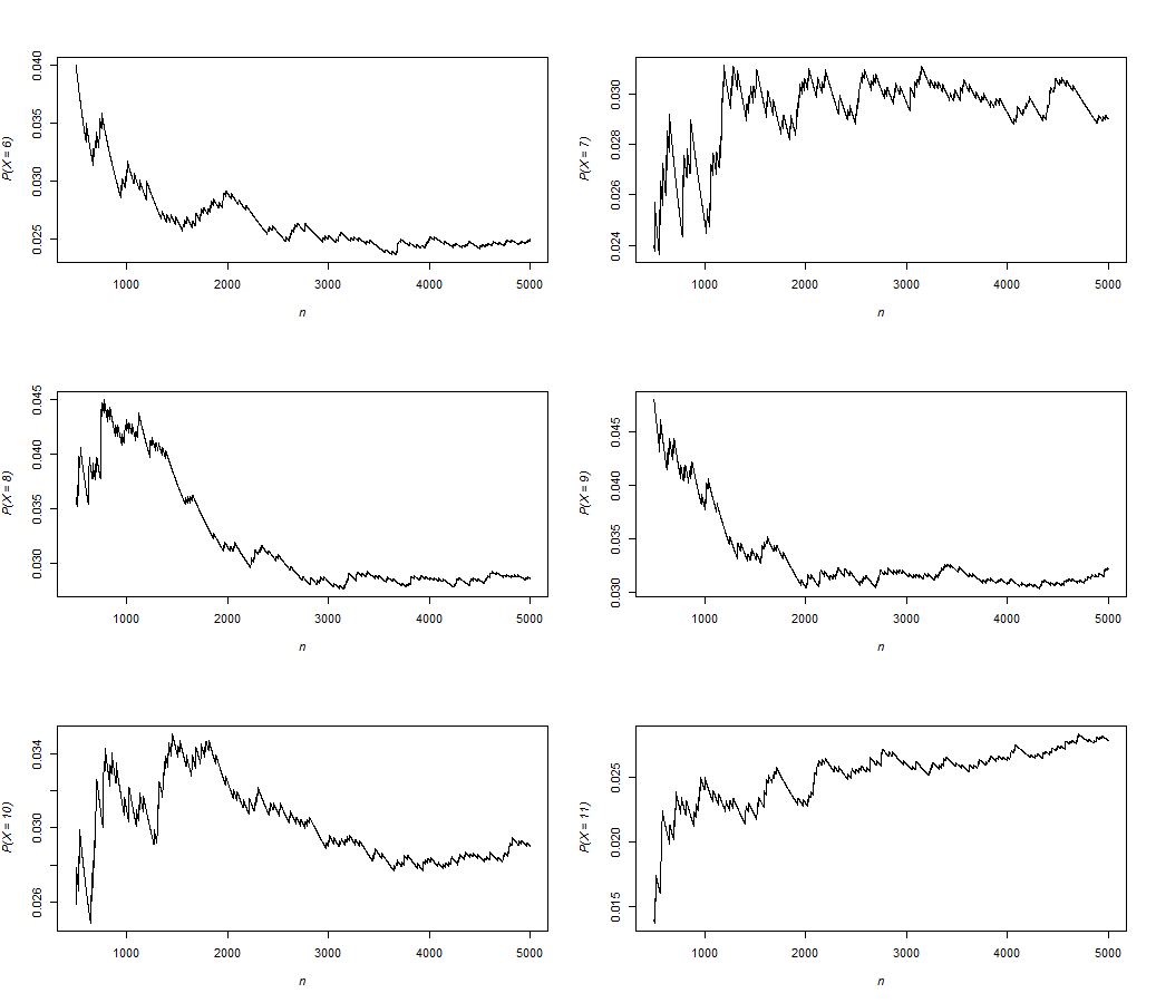
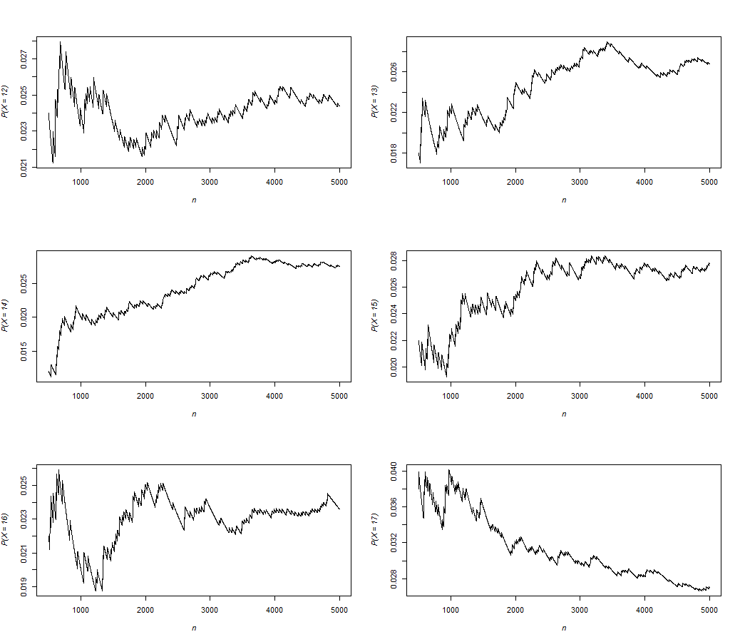
In this section, it is presented the results of this research paper. First, it is shown the convergence probability of each number of the roulette wheel for the in-sample data analysis. Then, it is presented the backtesting results, for the in-sample data. Finally, it is applied the walk-forward optimization in order to assess the profitability of the strategy.



| Outcome | Probability | Mean | St. Dev |
|---|---|---|---|
| 0 | 2.84% | 2.74% | 0.18% |
| 1 | 2.76% | 2.82% | 0.28% |
| 2 | 2.84% | 2.67% | 0.21% |
| 3 | 2.64% | 2.43% | 0.17% |
| 4 | 2.60% | 2.60% | 0.13% |
| 5 | 2.44% | 2.50% | 0.11% |
| 6 | 2.50% | 2.67% | 0.29% |
| 7 | 2.90% | 2.94% | 0.14% |
| 8 | 2.86% | 3.22% | 0.50% |
| 9 | 3.22% | 3.33% | 0.36% |
| 10 | 2.90% | 3.30% | 0.21% |
| 11 | 2.78% | 2.51% | 0.21% |
| 12 | 2.44% | 2.51% | 0.11% |
| 13 | 2.68% | 2.48% | 0.29% |
| 14 | 2.76% | 2.41% | 0.40% |
| 15 | 2.78% | 2.59% | 0.22% |
| 16 | 2.36% | 2.30% | 0.13% |
| 17 | 2.70% | 3.14% | 0.35% |
| 18 | 2.32% | 2.08% | 0.27% |
| 19 | 2.44% | 2.24% | 0.17% |
| 20 | 2.96% | 3.03% | 0.20% |
| 21 | 2.56% | 2.25% | 0.26% |
| 22 | 3.08% | 3.36% | 0.24% |
| 23 | 2.86% | 3.31% | 0.58% |
| 24 | 2.72% | 2.78% | 0.15% |
| 25 | 2.86% | 2.76% | 0.16% |
| 26 | 2.62% | 2.58% | 0.11% |
| 27 | 2.66% | 2.75% | 0.19% |
| 28 | 2.60% | 2.51% | 0.29% |
| 29 | 2.98% | 3.21% | 0.21% |
| 30 | 2.86% | 2.98% | 0.16% |
| 31 | 2.56% | 2.73% | 0.17% |
| 32 | 2.70% | 2.68% | 0.10% |
| 33 | 2.42% | 2.29% | 0.30% |
| 34 | 2.48% | 2.46% | 0.15% |
| 35 | 2.74% | 2.69% | 0.17% |
| 36 | 2.58% | 2.56% | 0.16% |
As we can see, the numbers that has higher probability of occurrence in the sample of 5,000 spins are: 9, 22 and 29; with probabilities of , and respectively.
It has also been found, that the probability of occurrence of the roulette wheel numbers seems to follow an stochastic process and, in some specific cases, the way they converge to its mean are more stable than other numbers. This is the case for numbers such as: 1, 6, 8, 9, 17 and 23, which coincidently, are the numbers with higher standard deviations than the other ones: , , , , and respectively.
We can try to model this stable convergence to the mean as a mean-reverting process, with an Ornstein-Uhlenbeck process, which is commonly used in quantitative finance to model interest rates [16], [17], [18].
As the number with the highest probability of occurrence is the number we will use it to try to model the way its probability evolve over time. We define the following stochastic differential equation as:
| (29) |
Where is the process of over a time interval . In the RHS, the term is deterministic, and the coefficient of is know as the drift of the process; the other term is random. The coefficient of is known as the diffusion of the process, where follows a standard Wiener process. This can be written in integral form as:
| (30) |
From this, we can begin to state our Ornstein-Uhlenbeck process as:
| (31) |
Where , and are parameters. This can be integrated from to with the auxiliary function to:
| (32) |
The expression from above can be simplified as:
A set of 1,000 Monte Carlo simulations are performed in Mathematica for the Ornstein-Uhlenbeck process described in (31), in order to model the probability of occurrence of the number 9 :

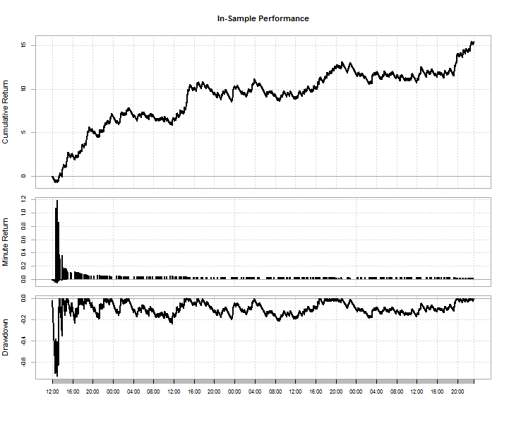
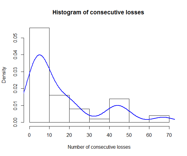
Despite the fact that the roulette wheel is not statistically biased due to a Chi square test, where is less than with degrees of freedom and confidence level, we can still have profits if we select only the numbers that pass the filter of greater or equal than three percent of probability of occurrence, which in this case are the numbers 9 and 22. Moreover, we will compare the performance of a flat betting system (FBS) against Kelly. The wager’s size for each FBS are defined as the average of all Kelly’s position size in each Walk-Forward Optimization. An initial capital of was selected arbitrary in order to assess the statistical properties of the strategy.
For this in-sample backtesting we can see the presence of curve fitting which is evident in the distribution of the returns figure from above. This issue is generated because the strategy was designed and over-optimized to this specific data set, i.e. a good metaphor would be: buying a lottery ticket with a previous knowledge of the winning numbers. In order to avoid curve fitting issues and test if our strategy it is robust we will use the tool of walk-forward optimization. The results from the walk-forward optimization and backtesting are presented in the same way as the back-tester used in Bloomberg L.P.’s software as follows:
| Number of obs. | 5000 |
|---|---|
| Wins | 315 |
| Losses | 4685 |
| P&L | 29,979.14 |
| % P&L | 1,498.96 |
| Total Wins | 199,710 |
| Total Losses | 169,730.9 |
| Avg. Win | 634 |
| Avg. Loss | 36.22 |
| Max. Win | 634 |
| Max. Loss | 36.22 |
| Max. Drawdown | 5,053.89 |
| Calmar Ratio | 5.93 |

| Statistics | Kelly Criterion | Flat wager |
|---|---|---|
| Number of obs. | 2479 | 2479 |
| Wins | 84 | 84 |
| Losses | 2395 | 2395 |
| P&L | 6,839.57 | 16,790.21 |
| % P&L | 341.98 | 839.51 |
| Total Wins | 81,066.99 | 90,741,23 |
| Total Losses | 74,218.33 | 73,920.15 |
| Avg. Win | 965.08 | 1080.25 |
| Avg. Loss | 30.99 | 30.86 |
| Max. Win | 1,726.00 | 1080.25 |
| Max. Loss | 57.16 | 30.86 |
| Max. Drawdown | 7,167.49 | 5,524.72 |
| Calmar Ratio | 0.95 | 3.04 |


| Statistics | Kelly Criterion | Flat wager |
|---|---|---|
| Number of obs. | 499 | 499 |
| Wins | 24 | 24 |
| Losses | 475 | 475 |
| P&L | -1,992.21 | -1,053.43 |
| % P&L | -99.61 | -52.67 |
| Total Wins | 7,012.65 | 7,900.69 |
| Total Losses | 8,934.38 | 8,935.304 |
| Avg. Win | 292.19 | 329.20 |
| Avg. Loss | 18.81 | 18.81 |
| Max. Win | 1,294.00 | 329.20 |
| Max. Loss | 119.60 | 18.81 |
| Max. Drawdown | 3,384.99 | 2,238.53 |
| Calmar Ratio | -0.59 | -0.47 |


| Statistics | Kelly Criterion | Flat wager |
|---|---|---|
| Number of obs. | 501 | 501 |
| Wins | 33 | 33 |
| Losses | 468 | 468 |
| P&L | -1,269.61 | 5340.02 |
| % P&L | -63.48 | 267.00 |
| Total Wins | 22,170.33 | 28,422.68 |
| Total Losses | 23,368.93 | 23,033.45 |
| Avg. Win | 671.83 | 861.29 |
| Avg. Loss | 49.93 | 49.22 |
| Max. Win | 2,181.00 | 861.29 |
| Max. Loss | 202.10 | 49.22 |
| Max. Drawdown | 5,433.79 | 4,084.99 |
| Calmar Ratio | -0.23 | 1.31 |


| Statistics | Kelly Criterion | Flat wager |
|---|---|---|
| Number of obs. | 365 | 365 |
| Wins | 23 | 23 |
| Losses | 342 | 342 |
| P&L | -1,459.41 | 2,528.17 |
| % P&L | -72.97 | 126.41 |
| Total Wins | 13,330.28 | 17,102.31 |
| Total Losses | 14,718.25 | 14,531.65 |
| Avg. Win | 579.58 | 743.58 |
| Avg. Loss | 43.04 | 42.49 |
| Max. Win | 1572.00 | 743.58 |
| Max. Loss | 145.90 | 42.49 |
| Max. Drawdown | 3,714.64 | 2,273.23 |
| Calmar Ratio | -0.39 | 1.11 |


| Statistics | Kelly Criterion | Flat wager |
|---|---|---|
| Number of obs. | 492 | 492 |
| Wins | 23 | 23 |
| Losses | 469 | 469 |
| P&L | -1,994.70 | -899.51 |
| % P&L | -99.73 | -44.98 |
| Total Wins | 4,327.74 | 5,263.73 |
| Total Losses | 6,250.95 | 6,249.91 |
| Avg. Win | 188.16 | 233.21 |
| Avg. Loss | 13.33 | 13.33 |
| Max. Win | 1,222.00 | 233.21 |
| Max. Loss | 113.50 | 13.33 |
| Max. Drawdown | 3,170.51 | 1,359.26 |
| Calmar Ratio | -0.63 | -0.66 |


| Statistics | Kelly Criterion | Flat wager |
|---|---|---|
| Number of obs. | 759 | 759 |
| Wins | 47 | 47 |
| Losses | 712 | 712 |
| P&L | -1,892.20 | 686.10 |
| % P&L | -94.61 | 34.31 |
| Total Wins | 2,714.65 | 5,153.59 |
| Total Losses | 4,537.08 | 4,461.22 |
| Avg. Win | 57.76 | 109.65 |
| Avg. Loss | 6.37 | 6.26 |
| Max. Win | 316.70 | 109.65 |
| Max. Loss | 67.34 | 6.26 |
| Max. Drawdown | 1,924.77 | 626.58 |
| Calmar Ratio | -0.98 | 1.10 |


| Statistics | Kelly Criterion | Flat wager |
|---|---|---|
| Number of obs. | 885 | 885 |
| Wins | 50 | 50 |
| Losses | 835 | 835 |
| P&L | -1,994.323 | 594.66 |
| % P&L | -99.72 | 29.73 |
| Total Wins | 10,944.32 | 13,341.75 |
| Total Losses | 12,868.84 | -12,731.84 |
| Avg. Win | 218.89 | 266.83 |
| Avg. Loss | 15.41 | 15.25 |
| Max. Win | 811.80 | 266.83 |
| Max. Loss | 74.72 | 15.25 |
| Max. Drawdown | 2,135.71 | 1913.59 |
| Calmar Ratio | -0.93 | 0.31 |
4 Conclusion
In this paper, we have seen that is not necessary that the roulette wheel has to be statistically biased in order to have profits in the short-term. Importantly, however, it is needed a probability of occurrence approximately to greater or equal than three percent for make a bet on a specific number.
Moreover, the probability of occurrence of each number at the roulette wheel can be modelled very accurately as an Ornstein-Uhlenbeck process. This result showed consistency with the Monte Carlo simulations shown in Figure 3. Further analysis is needed in order to assess if it is possible to make forecasts of how this probabilities evolve over time with this same model.
Furthermore, the flat betting system (FBS) has shown a better performance than the Kelly criterion’s system, due that Kelly’s carries higher volatility and it is more aggressive than the FBS, thus, as more losses in a row comes into the strategy it is more difficult for Kelly’s system to recover. It would be a matter of further study to assess the performance of half a Kelly criterion as a position size. Similarly, another matter of further study might involve perform a Non-anchored Walk-forward optimization, in order to get more up-to-date probabilities of occurrence and include the momentum factor of the roulette wheel into the strategy.
In addition, it has also been observed that roulette outcomes get less predictable over time, which may be an evidence of the Second Law of Thermodynamics, which states that disorder, known as entropy, increases with time.
5 Acknowledgements
This research paper would not have been possible without the support of the following people, whom I am grateful:
My family, in alphabetical order: my brother, father and mother. For their tremendous support in my personal life over time.
My ex-wife, for her big support during the five years of my undergraduate education and sharing those years of her life with me.
My three godsons, in alphabetical order: Anthony, César and Piero, for took the crazy decision of choosing me as their godfather.
Pedro Cornejo, mentor and friend who brought me into the financial industry, to whom I am deeply indebted.
Gabriel Chirre, for his loyal and disinterested friendship during my professional career.
David Hafermann, who taught me the concepts of backtesting and walk-forward optimization, and showed me the importance of programming.
Dennis La Cotera, a true Peruvian quant, who taught me the amazing properties of computational finance and applied mathematics in Wolfram Mathematica.
My professors at the CQF Institute, for sharing their great knowledge about quantitative finance with me.
My professors at Universidad San Ignacio de Loyola, who gave me the very first concepts of finance and econometrics at the Faculty of Economics.
In order of meeting to: Megija, Darja, Laura, Sigita and Jana, blackjack and roulette dealers at Evolution Gaming, for their invaluable motivational words that made this research paper possible. In this group, a very special thanks to Jana Zidere for verify in a daily basis my progress on this paper and for share the same crazy spirit as the author.
Above all, thanks to the Intelligent Designer.
6 References
[1] Pozdnyakov, Vladimir and Steele, Michael (2009). Martingale Methods for Patterns and Scan Statistics. Statistics for Industry and Technology. pp. 289-317
[2] Farmer, Doyne and Sidorowich John (1987). Predicting Chaotic Time Series. Physical Review Letters. Vol 59, No. 8.
[3] Small, Michael and Tse, Chi Kong (2012). Predicting the outcome of roulette. Chaos: An Interdisciplinary Journal of Nonlinear Science
[4] Jirina, Miroslav (1978). A biased roulette. Annales de l’Institute Henri Poincaré. Vol 14, No 1, p. 1-23.
[5] Sundali, James and Croson, Rachel (2006). Biases in casino betting: The hot hand and the gambler’s fallacy. Judgement and Decision Making. Vol. 1, No. 1, pp. 1-12.
[6] Ethier, S.N. (1982). Testing for favourable numbers on a roulette wheel. Journal of the American Statistical Association. Vol. 77, No. 379, pp. 660-665.
[7] Etemadi, N. Z. (1981). An elementary proof of the strong law of large numbers. Zeitschrift für Wahrscheinlichkeitstheorie und Verwandte Gebiete. Vol. 55, Issue 1, pp. 119-122.
[8] Ni, Jiarui and Zhang, Chengqi (2005). An Efficient Implementation of the Backtesting of Trading Strategies. Lecture Notes in Computer Science. Vol. 3758, pp. 126-131.
[9] Dixon M., Klabjan, D. and Bang, J. (2015). Backtesting Trading Strategies with Deep Neural Networks on the Intel Xeon Phi. SSRN Electronic Journal.
[10] Wong. W (2008). Backtesting trading risk of commercial banks using expected shortfall. Journal of Banking and Finance. Vol, 32, Issue 7, pp. 1404-1415.
[11] Menkveld, Albert J. (2013). High frequency trading and the new market makers. Vol. 16, Issue 4, pp. 712-740.
[12] Schneider, D. (2011). Trading at the speed of light. IEEE Spectrum. Vol. 48, Issue 10, pp. 11-12.
[13] Scholtus M., and Dijk D. (2012). High-Frequency Technical Trading: The Importance of Speed. Tinbergen Institute Discussion Paper. p. 63.
[14] Kelly, John L. Jr. (1956). A New Interpretation of Information Rate. Bell Systems Technical Journal. Vol. 35, pp. 917-926.
[15] Young, T. (1991). Calmar Ratio: A Smoother Tool. Future Magazine. Vol. 20, Issue 1, p. 40.
[16] Barndorff-Nielsen, O. and Shephard, N. (2001). Non-Gaussian Ornstein-Uhlenbeck-Based models and some of their uses in financial economics. Journal of the Royal Statistical Society. Series B (Statistical Methodology) Vol. 63, Issue 2, pp. 167-241.
[17] Maller R., Müller G. and Szimayer A. (2009). Ornstein-Uhlenbeck Processes and Extensions. Handbook of Financial Time Series. Issue 1930, pp. 421-437.
[18] Önalan, Ö. (2009). Financial Modelling with Ornstein-Uhlenbeck Processes Driven by Lévy Process. Lecture Notes in Engineering and Computer Science. Vol. 2177, Issue 1, pp. 1350-1355.