Referential Uncertainty and Word Learning in High-dimensional, Continuous Meaning Spaces

Michael Spranger Affiliation: Sony Computer Science Laboratories Inc., Tokyo, Japan
Email: michael.spranger@gmail.com Katrien Beuls Affiliation: Vrije Universiteit Brussel, Brussels, Belgium
Email: katrien@ai.vub.ac.be

Abstract

This paper discusses lexicon word learning in high-dimensional meaning spaces from the viewpoint of referential uncertainty. We investigate various state-of-the-art Machine Learning algorithms and discuss the impact of scaling, representation and meaning space structure. We demonstrate that current Machine Learning techniques successfully deal with high-dimensional meaning spaces. In particular, we show that exponentially increasing dimensions linearly impact learner performance and that referential uncertainty from word sensitivity has no impact.

I Introduction

The most important aspect of word learning is often thought to be referential uncertainty. Quine [1] famously framed referential uncertainty as a general problem everybody faces when trying to learn an unknown language. Suppose an anthropologist studies an isolated tribe. When members of the tribe see a rabbit, they shout “gavagai”. The anthropologist hears the word for the first time and has no idea what the word means. In principle the meaning of the word could be anything from perceptual features of objects present (or not present!), features of the environment, social and historical facts etc. The space of possible meanings is essentially infinite and the question is how the anthropologist can solve this puzzle.

Many researchers claim that children face the same problem when trying to learn language. Models that deal with word learning try to capture referential uncertainty in various ways. Schematically, we can distinguish between the following approaches to meaning and corresponding models (see Fig. 1).

Word-Object Mapping Models (WOM)

Some models approach word learning as a discrete mapping problem from words to object, e.g. [2, 3]. How difficult the mapping problem is depends on factors such as the number of objects in the context of an interaction or the feedback given by the caregiver. If there is only one object, then the mapping can be learned instantaneously and no problem exists. If there are multiple objects, then referential uncertainty does exist if there is ambiguous, unreliable or no feedback from the caregiver.

Fig. 1: Left: models of word-object mappings learn associations between words and a priori known objects. Middle: symbolic feature based models learn associations to symbolic feature representations. Right: word meanings are organizations of

n

dimensional, continuous feature vectors.

Combinations of Feature Models (CFM)

Some researchers [4, 5, 6] have modeled word meaning as combinations of symbolic features. The features themselves are known prior to word learning. In CFM the meaning space is as large as all possible combinations of features. The meaning space grows combinatorially with the number of features. There are fundamental differences between WOM and CFM. In CFM, a word can be linked to multiple features. The learner upon hearing a word and seeing a single object cannot know which features of the object the word refers to. Consequently, referential uncertainty can occur in single object contexts This is different from WOM, where referential uncertainty is exclusively related to the number of objects in the context.

Continuous Meaning Space Models (CMS)

Few models address the learning of words related to representations in continuous vector spaces [7, 8]. The problem of referential uncertainty in continuous meaning spaces is large and depends chiefly on the number of objects in a learning context, the number of dimensions of meaning vectors and whether or not objects can refer to subspaces of the meaning space (color space etc). In that sense CMS behave similar to CFM. The difference to CFM is that the meaning space is an infinite continuous vector space by default.

The few available CMS models are often shown to work in low-dimensions and with few words. In this paper we survey the state of the art in word learning algorithms for high-dimensional continuous meaning spaces with referential uncertainty caused by words referring to features of objects (rather than caused by multiple objects in the context). As it turns out, this problem has been dealt with in the Machine Learning (ML) community. We first analyze the problem of word learning from the viewpoint of machine learning in $n$ -dimensional spaces. We then test various state-of-the-art ML methods on simulated and grounded data sets, analyze dynamics of online learning and the impact of various referential uncertainty. Lastly, we discuss how all this fits in the general landscape of language learning models.

II Description Games

One interaction pattern (game) often used in models of word learning is the description game (DG). The basic structure of DG is the following. The learner observes a particular situation (context) of $l$ objects ( $l=1$ for this paper) and also observes $k$ words uttered by the tutor ( $k=5$ for this paper). So for instance, both learner and tutor observe one object. The tutor says “block, bright, red,..,..” (order does not matter). The learner then has to learn the meaning of these words by integrating information over various trials. The success of the learner is measured by testing which words the learner produces for objects and how this overlaps with the production of words of the tutor.

An important aspect of these games is the tutor strategy - the representation and algorithm the tutor uses for producing $k$ words for an object. In this paper, objects are represented by $n$ dimensional feature vectors $o\in[0,1]^{n}$ . The tutor represents each word using a prototype $p\in[0,1]^{n}$ and a weight vector $w\in[0,1]^{n}$ . Prototypes for tutors are randomly drawn from a uniform distribution $\mathrm{U}(0,1)^{n}$ . Weights are drawn from a binomial distribution $\mathrm{B}(1,0.5)^{n}$ . If a weight vector is all 0 we randomly set one of the weights to 1.

For an object $o\in[0,1]^{n}$ the tutor first computes a weighted Euclidean distance $\operatorname{wd}$

\operatorname{wd}_{w,p}(o)=\sqrt{\sum_{i=1}^{n}w_{i}(o_{i}-p_{i})^{2}}

The tutor then chooses the $k$ closest words for the description of an object, i.e.

\argmin_{w,p\in P}(\operatorname{wd}_{w,p}(o))

This representation and word production strategy has the following desirable properties. The strategy models feature dimension sensitivity of words/prototypes. For instance, there could be a word that is sensitive only to the brightness dimension. Other words could be sensitive to blue and red channels. Secondly, words are not produced uniformly - similar to human language. Some words are used often, others only occur few times in the training set. Lastly, the tutor produces $k$ words for any object. Together with the object distribution in $[0,1]^{n}$ this leads to interesting, non-linear interactions between words and objects.

Let us briefly examine the difficulty of the learning task. The learner has to learn to produce (predict) the same words as the tutor based on examples provided by the tutor. Suppose that $m=|W|$ denotes the number of words the tutor knows. In principle, chance performance is equal to choosing $k$ out of $m$ words without repetition and order does not matter. For experiments with $k=5$ and $m=100$ this amounts to ${100\choose 5}=75,287,520$ assuming a uniform distribution of words.

III Description Games and Machine Learning

In machine learning terms, DG is a supervised, multi-class (multiple words), multi-label (multiple words per object), online classification problem. There is an immense literature and an abundance of algorithms that can be tested on this problem [9, 10].

For this paper, we test roughly a dozen different learning methods from linear models, to ensemble classifiers, Bayesian learning and neural networks that solve the description game learning problem. The following paragraphs give a (brief) overview of the various methods we tested.

Nearest neighbor (NN)

One of the simplest and often best performing methods is nearest neighbor - also called KNN or in this paper KNeighbors [11] . KNeighbors is a non-parametric method that stores all samples ever encountered. New samples are classified based on the class of its $k$ nearest neighbor (stored examples). The algorithms simplicity and the (often out of the box) success of this method have led to its widespread adoption.

We also use a related algorithm from the same family: Nearest Centroid (NC). NC represents classes using centroids of corresponding samples. New samples are classified based on the shortest distance to centroids. This method is among the most widely used in word learning because it corresponds nicely with ideas in psychology [12].

Generalized Linear Models (GLM)

GLM describe a family of algorithms that all model predictions as linear combinations of input variables. All models furthermore assume that predictions (dependent variables) are generated from exponential probability distributions (Gaussian, binomial, gamma etc). Learners also differ in terms of regularization and learning regime (closed-form, stochastic etc). We are using various classifiers: Logistic Regression, Online Passive Aggressive (PA) [13] and Stochastic Gradient Descent (SGD) [14].

Ensemble methods (ENM)

ENM are meta algorithms that try to improve classification results by combining results of sets (ensembles) of classifiers (NN, linear or others). There are basically two types of ensemble methods. The first relies on weak, underfitting classifiers each often only slightly better than random choice. There are two main methods in this group: AdaBoost [15] and Gradient Boosting [16]. AdaBoost works by fitting a series of weak learners. Each step (boosting iteration), training data is weighted to focus on samples that are not correctly classified in the previous step. Successive classifiers therefore essentially encode classification for various aspects of the data. New samples are classified by computing the majority estimates of classifiers. Gradient Boosting is an extension of boosting for optimizing any differentiable loss function.

Another class of ensemble methods takes the opposite approach and relies on sets of classifiers that are complex, over-fitting classifiers. Here, we use Random Forest [17] and Extra Trees [18], which use ensembles of decision trees. Decision trees are a non-parametric method that learns binary decisions (nodes) and arranges them in a binary tree [19]. Both RandomForest and ExtraTrees build multiple overfitting classifiers on random subsets of samples and features.

Bayesian Methods (BM)

BM rely on Bayes theorem to transform the classification problem into one of estimating probability distributions. New samples are classified based on prior probabilities of classes, as well as posterior estimates of sample probabilities and the probability of observing samples given classes. Bayesian classifiers primarily differ in the assumptions they make for the probability distributions that need to be estimated. We use Gaussian Naive Bayes classifiers [20] (normal distributions, independent features) and Multinomial Naive Bayes (multinomial distributions, independent features). Parameters for probability distributions are estimated using expectation-maximization.

Neural networks (NN)

Recently neural networks have pushed the state-of-the-art in many classification problems such as face recognition, image labeling etc. The current trend is to stack multiple layers of neurons (mostly non-linear functions) and train them (often one layer at a time) using variants of the backpropagation algorithm. NN can take various forms in terms of network topologies, transfer functions, training regimes and learning rules. For the purpose of this paper, we used a multi-layer perceptron (MLP) - (2 layers, rectified linear units, with a final sigmoid layer for classification).

Refer to caption — Fig. 2: Objects used in evaluating different algorithms.

IV Experimental Setup

IV-A Datasets

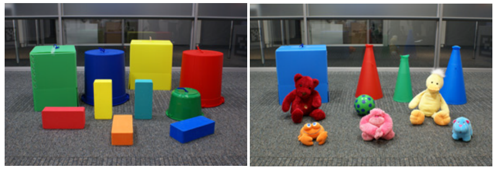
We compare different learners on simulated and robot data sets. The robot data sets consists of 20 different objects (see Figure 2) of various color, shape, size. We recorded approximately 1000 scenes in which two robots observe objects from different perspectives. Scenes differ in the positions of objects, which also alters objects’ perceived shape and color features. For each object $n=17$ feature dimensions are extracted: x, y, z position, YUV color values (mean min, max), width, height, length. Data is scaled between 0 and 1 using a linear scaler and for some classifiers to zero mean, unit variance.

GRO1

This dataset consists of all object observations ever made by the two robots in one matrix ( $4532\times 17$ ). GRO1 is used to experiment, with tutor and learner having the same object perception, in particular, the same feature estimation for objects.

GRO2

This dataset is a grounded robot data set. It consists of two matrices. One for each robot (two matrices of size $4532\times 17$ ). Each row corresponds to the perception of the same physical object from the viewpoint of the two different robots. This data is used in the following way. The tutor produces words from the perspective of robot 1 (matrix 1). The learner learns from the observation of the same object but from perspective of the other robot (matrix 2). GRO2 is used to evaluate what happens if there is perceptual deviation [21]. That is tutor and learner see the scene from different viewpoints and therefore have different feature estimations for objects. For instance, the tutor robot might observe different x, y positions for an object, since he sees the object from a different perspective. But also color and shape features will be slightly different.

SIM

This dataset is simulated and consists of 4532 object observations of $n=17$ feature dimensions drawn from a uniform distribution $\mathrm{U}(0,1)$ .

IV-B Methods

Learners are trained on samples of objects and one-hot vector encoded words produced by the tutor. Each classifier has to predict (produce) the correct set of $k$ words given (new) vectors of objects by predicting a one-hot vector encoding of word activations. We then measure the difference between the production of the tutor and the prediction of the learner. For learning algorithms that predict probabilities $p$ for words (e.g. MLP), if $p>0.5$ then the word is counted as a prediction.

For all experiments here, we draw $|W|=100$ prototypes and weights for the tutor (according to the description in Section II) and perform 4-fold validation on data sets each consisting of 4532 samples. This means that training happens on roughly 3400 samples and testing on 1100 new samples. In summary, the standard parameters for our evaluations are $n=17$ (number of features), $|W|=100$ (number of words and prototypes tutor), $k=5$ (number of words uttered by the tutor) and $p=0.5$ (for the binomial distribution of tutor weights).

Classifiers not supporting multi-class, multi-label by default were trained using one-vs-rest [22]. The exception are RandomForest, KNeighbors, NearestCentroid and MLP. Most classifiers rely on various hyper-parameters. We optimized hyper-parameters using parameter grid searches on a separate simulated dataset SIM-DEVELOP (same characteristics as SIM). Hyper-parameters were optimized once on SIM-DEVELOP and then fixed for all results reported here.

IV-C Measures

In this paper we use a single performance measure: f-score [23]. F-score is defined as the harmonic mean of precision and recall. There are various definitions of precision and recall depending on the classification problem (binary, multi-class, multi-label). Generally speaking, precision measures the amount of wrong words per sample found by the learner. Recall measures how many of the correct words were predicted by the learner. We use a particular f-score measure which is called example-based (or sample) that does not take into account unbalanced word distributions. An f-score of 100 means that all words and only those words uttered by the tutor are uttered by the learner.

V Results

	SIM	GRO1	GRO2
Nearest Neighbor
KNeighbors	67.89	74.06	61.25
NearestCentroidOvR	65.81	83.44	63.87
Linear Models
SGD	79.49	87.93	65.27
PassiveAggressive	63.32	84.70	65.04
LogisticRegression	76.61	86.17	61.95
Ensemble Methods
RandomForest	80.84	87.91	65.79
ExtraTrees	67.89	74.06	61.25
AdaBoost	79.49	87.93	65.27
GradientBoosting	80.83	92.58	65.68
Bayesian
GaussianNB	63.85	84.44	65.25
MultinomialNB	75.35	87.02	67.64
Neural
MLP	82.74	91.58	70.87

TABLE I: Results comparison grounded and simulated data (sample-based f-score,

n=17

k=5

p=0.5

|W|=100

)

Table I shows the performance of various classifiers on grounded and simulated data. Many learners perform well on the task with respect to task complexity. In particular, simple algorithms such as GaussianNB or linear models perform well. More complex methods such as ensemble methods generally are top performers. The best performing method on SIM and GRO2 is the multi-layer perceptron MLP. On GRO1 GradientBoosting is the front runner. Although ensemble methods generally perform quite similar. None of the methods fail catastrophically, which is mostly due to hyper-parameter optimization.

Interestingly all methods improve on grounded data (GRO1) some by as much as 20 points (e.g. PassiveAgressive). This suggests that methods are able to take advantage of structure available in grounded data. However, all methods perform worse on GRO2 than on GRO1. In some cases performance differs by almost 30 points between GRO2 and GRO1.

A word on how to understand these results. This study focusses on understanding the baseline for word learning in high-dimensional meaning spaces. These results are existence proofs (lower bounds) showing that learners can solve this problem with relatively high f-score. These results do not show limits of individual learning algorithms, rather results show general trends that hint at the scope of the learning problem.

V-A Scaling Object Feature Dimensions

We are interested in understanding referential uncertainty in high-dimensional meaning spaces. Consequently, we manipulated the number of dimensions of object features $n$ . The number of dimensions in the grounded data sets is fixed by the vision system, so we increased the number of dimensions for simulated data. All other parameters are kept the same. Figure 3 shows how classifiers do for $n\in\{10,100,1000,10000\}$ .

Fig. 3: Performance of classifiers for increasing

n

(number of object feature dimensions) with

p=0.5

|W|=100

k=5

, data set size 4532, 4 fold.

Average performance across all classifiers degrades linearly with orders of magnitude of difference in $n$ for the best performing classifiers (MLP, AdaBoost). These results suggest that classifiers optimized for various $n$ and/or increasing the number of training samples, could actually deal with even higher $n$ -dimensional data (remember that all classifiers were optimized for $n=17$ ).

There is one classifier that performs poorly (MultinomialNB) all along, while others (e.g. ExtraTrees, RandomForest) degrade much more rapidly with number of dimensions than the best performing ones. Others perform best for certain $n$ (e.g. PassiveAggressive). All of these classifiers perform reasonably well or very well on the hyper-parameter optimized $n=17$ . Consequently, these classifiers are sensitive to hyper-parameters with respect to number of dimensions.

V-B Scaling Word Sensitivity

Another dimension of scaling is the sensitivity of words. Prototype weights for all experiments reported so far were drawn from a binomial distribution $\mathrm{B}(1,p=0.5)$ . This means that words are on average sensitive to half of the dimensions. In our experiments, referential uncertainty is tied to the fact that words can refer to aspects of objects. To test learners, we ran experiments for various $p\in\{0.1,0.25,0.5,0.75,1.0\}$ and $n=100$ . All other parameters stay the same.

Figure 4 shows that quite a few learners (AdaBoost, ExtraTrees, MLP etc) have absolutely no problem dealing with various $p$ . We can conclude that these learners will perform well on mixed languages where some words encompass all features of an object and some are more specific and only refer to certain features. Other learners such as KNeighbors become better with larger $p$ . This is no surprise since KNeighbors stores full examples.

Fig. 4: Performance of learners for varying values of

p\in\{0.1,0.25,0.5,0.75,1.0\}

with

n=100

|W|=100

and

k=5

V-C Online Learning

One important aspect in language learning from a developmental point of view is online learning. We tested how well the algorithms perform over time. For this we incrementally train classifiers on the training set. For instance, we train on the first $m$ object observations and evaluate the f-score on the test data set. Figure 5 shows the performance of classifiers over time. Pretty much all classifiers learn very fast with most of the gains happening on the first 500 training samples. In other words, the learner becomes quite sufficient after 500 interactions with the tutor. After 1000 training samples all classifiers are within 5 points of their final f-score.

These results for online learning are quite remarkable given that there are 100 words that need to be learned. Certainly, what helps here is that certain words will be used frequently and others less frequently. We analyzed results with respect to frequency of words and it becomes evident that this is indeed one big driver of the speed of learning.

Fig. 5: Online learning performance of various classifiers on simulated data.

V-D Discussion of Results

Our results show that many off-the-shelf machine learning algorithms can deal with high-dimensional meaning spaces. We only optimized classifiers for $n=17$ and we get linear drop in performance for exponential increase in number of dimensions. This suggest that we might be able to get on par performance even for very high $n$ - if we optimize classifiers for each $n$ and if we logarithmically increase training set size. Our results also show that many classifiers have no problem dealing with feature sensitivity related to referential uncertainty.

Our experiments suggest that referential uncertainty in high-dimensional meaning spaces is NOT an exponentially growing problem. In other words adding dimensions has at most a linear effect on learners in the paradigm discussed here. This is an interesting result because it suggests that referential uncertainty although often thought of as an exponentially growing problem with the number of dimensions or the degree with which words can associate to aspects of objects is much less of an issue than one might expect.

Meaning Space Structure

There is a difference in performance between SIM and GRO1 data sets. The reason is that there is much more structure in the real world than in the simulated world. The real world data sets consist of limited sets of objects that make up very defined spaces in the perceptual data space. For instance, there are certain clearly separable color regions based on the objects in GRO1. This structure in the environment helps all learning algorithms in becoming more successful.

Tutoring

Tutoring strategies are often thought to be about social feedback (e.g. pointing or agreement). But tutoring can also mean that the tutor is structuring the environment (and possibly also the language) for the learner. This can include taking perspective or conceptualizing the world from the viewpoint of the learner. Generally speaking it has been found that tutoring strategies help learners [8, 24]. The delta in performance between GRO1 and GRO2 confirms these ideas. In GRO1 the tutor will utter words based on what the learner sees. In GRO2 that is not the case. All classifiers perform less well on GRO2.

Unbalanced data

Another aspect that affects performance is the fact that training of words is unbalanced. There are some words that occur often and others that don’t (in fact some words do not even appear in the training set and only in the test set). The classifiers have difficulties with sparsely used words. Something that becomes apparent when examining macro-averaged f-scores (not reported here). This is often much lower than micro-averaged f-scores. This split suggests that (generally speaking) learners are good in learning frequent words but less good in learning less frequent words.

Representation

It is interesting to analyze various learning algorithms with respect to whether they actually build representations similar to that of the tutor. We deliberately chose various algorithms none of which directly tried to replicate the tutor behavior in the learner by learning the same representation. The tutor operates using weighted feature distances to prototypes. Words are only sensitive to a particular feature channel (e.g. the brightness). Algorithms such as KNeighbors do not explicitly represent information like that. They just collect samples. Others such as RandomForrest do actually learn how to distinguish different words based on explicitly learning which features matter with respect to the word. An interesting result of this study is that both of these algorithms perform comparably well in terms of replicating the tutors behavior. But if we look at different $p$ value experiments, we can see that discriminative feature learners such as AdaBoost outperform KNeighbors.

VI Related Work

Referential uncertainty

There is an important difference between the setup here and other studies. Many studies are concerned with enumerable objects in context and how this leads to referential uncertainty (see [25, 7, 5] among others). In this paper, we use referential uncertainty closer to Quine’s formulation and early studies by Siskind [4]. Quine focusses on aspects of a situation and not on enumerable objects as the source of referential uncertainty. In that sense the problem in Quine is larger. Even if you know the referent, the learner still knows nothing about the aspect of the referent the word refers to (color, shape etc). The question remains which referential uncertainty problem is solved by children (possibly both).

Description vs Discrimination

An important distinction between various models is the tutoring strategy - representation and algorithm for word production in the tutor. In description games, the speaker minimize distances between the topic object and words (here weighted Euclidean distances). In other types of interaction (called guessing games), the function being maximized for each word is the difference between the topic object $t$ and all the other objects (or features) in the context. An interesting question is whether different production strategies require different learning algorithms or not. Often the learner is modeled after the tutor and both use the same production and interpretation algorithms (see [8, 6] for some recent examples). This obviously biases the system and the question is whether this is necessary. What we can say for the models described in this paper is that nowhere did we bias the learners explicitly towards a particular production algorithm. Rather all that happens is that the learner is trying to replicate the tutor behavior.

Child Learning Strategies

Researchers in child language acquisition have provided many ideas about strategies that children use to learn the meaning of words. Some of them such as perceptual biases [26] could potentially be exploited by learning algorithms - if the language affords it. That is, if the language to be learned is based on salient perceptual distinctions then algorithms that learn discriminative features (e.g. decision trees, ensemble methods) can take advantage of that. Other child language learning strategies based on linguistic constraints [27] are not by definition part of the learning paradigm discussed in this paper. We only focus on unordered sets of words uttered by the tutor. The impact of strategies such as mutual exclusivity [28] and contrast [29] on the learning problem defined in this paper is subject to future work.

VII Conclusion

Abstract models can be used to answer questions about what algorithms children use to learn language. This is often done by trying to replicate empirical data. Another goal of models is to grasp the essence of the learning problem, characterize how hard it is and how the best known algorithms perform. This paper addresses aspects of the second goal. We defined an abstract version of the word learning problem, translated it to Machine Learning and compared state of the art methods on the problem. This establishes a baseline that can be used to understand word learning from the viewpoint of complexity.

Source code as well as data sets are published online at https://github.com/mspranger/icdl2016language.

References

[1] W. V. O. Quine, Word and object. MIT press, 2013.
[2] J. Fontanari, V. Tikhanoff, A. Cangelosi, R. Ilin, and L. Perlovsky, “Cross-situational learning of object–word mapping using neural modeling fields,” Neural Networks, vol. 22, no. 5, pp. 579–585, 2009.
[3] G. Kachergis, C. Yu, and R. M. Shiffrin, “An associative model of adaptive inference for learning word–referent mappings,” Psychonomic bulletin & review, vol. 19, no. 2, pp. 317–324, 2012.
[4] J. M. Siskind, “A computational study of cross-situational techniques for learning word-to-meaning mappings,” Cognition, pp. 39–91, 1996.
[5] J. De Beule, B. De Vylder, and T. Belpaeme, “A cross-situational learning algorithm for damping homonymy in the guessing game,” in Artificial Life X. MIT Press, 2006, pp. 466–472.
[6] P. Wellens, “Coping with combinatorial uncertainty in word learning: A flexible usage-based model,” in The Evolution of Language: Proceedings of the 7Th International Conference. World Scientific, 2008, p. 370.
[7] T. Belpaeme and A. Morse, “Word and category learning in a continuous semantic domain: comparing cross-situational and interactive learning,” Advances in Complex Systems, vol. 15, 2012.
[8] M. Spranger, “Grounded lexicon acquisition - case studies in spatial language,” in Development and Learning and Epigenetic Robotics (ICDL-Epirob). IEEE, 2013, pp. 1–6.
[9] M.-L. Zhang and Z.-H. Zhou, “A review on multi-label learning algorithms,” Knowledge and Data Engineering, IEEE Transactions on, vol. 26, no. 8, pp. 1819–1837, 2014.
[10] G. Tsoumakas, I. Katakis, and I. Vlahavas, “Mining multi-label data,” in Data mining and knowledge discovery handbook. Springer, 2009.
[11] T. M. Cover and P. E. Hart, “Nearest neighbor pattern classification,” Information Theory, IEEE Transactions on, vol. 13, 1967.
[12] E. Rosch, “Cognitive representations of semantic categories,” Journal of Experimental Psychology: General, vol. 140, pp. 192–233, 1975.
[13] K. Crammer, O. Dekel, J. Keshet, S. Shalev-Shwartz, and Y. Singer, “Online passive-aggressive algorithms,” The Journal of Machine Learning Research, vol. 7, pp. 551–585, 2006.
[14] L. Bottou, “Large-scale machine learning with stochastic gradient descent,” in Proceedings of COMPSTAT’2010. Springer, 2010.
[15] Y. Freund and R. E. Schapire, “A desicion-theoretic generalization of on-line learning and an application to boosting,” in Computational learning theory. Springer, 1995, pp. 23–37.
[16] J. H. Friedman, “Greedy function approximation: a gradient boosting machine,” Annals of statistics, pp. 1189–1232, 2001.
[17] L. Breiman, “Random forests,” Machine learning, no. 1, 2001.
[18] P. Geurts, D. Ernst, and L. Wehenkel, “Extremely randomized trees,” Machine learning, vol. 63, no. 1, pp. 3–42, 2006.
[19] L. Rokach and O. Maimon, Data mining with decision trees: theory and applications. World scientific, 2014.
[20] A. Jordan, “On discriminative vs. generative classifiers: A comparison of logistic regression and naive bayes,” Advances in neural information processing systems, vol. 14, p. 841, 2002.
[21] M. Spranger and S. Pauw, “Dealing with Perceptual Deviation - Vague Semantics for Spatial Language and Quantification,” in Language Grounding in Robots. Springer, 2012, pp. 173–192.
[22] N. Spolaôr, M. C. Monard, G. Tsoumakas, and H. D. Lee, “A systematic review of multi-label feature selection and a new method based on label construction,” Neurocomputing, 2015.
[23] M. Sokolova and G. Lapalme, “A systematic analysis of performance measures for classification tasks,” Information Processing & Management, vol. 45, no. 4, pp. 427–437, 2009.
[24] M. Spranger, “Incremental grounded language learning in robot-robot interactions - examples from spatial language,” in Development and Learning and Epigenetic Robotics (ICDL-Epirob). IEEE, 2015.
[25] M. Frank, N. D. Goodman, and J. B. Tenenbaum, “A bayesian framework for cross-situational word-learning.” in Advances in Neural Information Processing Systems, 2008, pp. 457–464.
[26] S. M. Pruden, K. Hirsh-Pasek, R. M. Golinkoff, and E. A. Hennon, “The birth of words: Ten-month-olds learn words through perceptual salience,” Child development, vol. 77, no. 2, pp. 266–280, 2006.
[27] L. Gleitman, “The structural sources of verb meanings,” Language acquisition, vol. 1, no. 1, pp. 3–55, 1990.
[28] E. M. Markman and G. F. Wachtel, “Children’s use of mutual exclusivity to constrain the meanings of words,” Cognitive psychology, 1988.
[29] E. V. Clark, “The principle of contrast: A constraint on language acquisition,” Mechanisms of language acquisition, vol. 1, p. 33, 1987.