On convexification/optimization of functionals including an $l^{2}$-misfit term

The article [18] is a condensed and improved version of this article, in which we denote $\mathcal{S}^{2}_{\gamma}$ by $\mathcal{Q}_{\gamma}$ and call it the quadratic envelope. This article still contains much more information, especially regarding computational aspects. We will not update notation/terminology in this article.

The purpose of this article is to convexify, or partially convexify, functionals of the type

where $x\in\mathbb{R}^{n}$, and

where $X\in\mathbb{M}_{m,n}$ (the space of $m\times n$-matrices with the Frobenius norm). In other words, we are interested in computing the lower semi-continuous (abbreviated l.s.c. ) convex envelope or at least an approximation thereof. We will also consider weighted norms and penalty terms like

in order to treat problems where a matrix of a fixed rank is sought. Such functionals appear in a multitude of optimization problems, where the goal is to find a point $x$ such that the functional attains its minimum, possibly with additional constraints on $x$. We refer to the overview article [50] which includes a long list of applications. The problem of minimizing (2) and (3) differ significantly in that (3) has a closed form solution whereas solving (2) is NP-hard. However, minimization of (3) over a subspace or in combination with additional priors, is also a hard well-known problem with many applications, and knowing the l.s.c. convex envelope can help to find approximate solutions, as we advocate in this paper. We refer to [32, 41] and the references therein for examples of applications.

Since the functional (4), as well as $\|\cdot\|_{0}$ and $\mathsf{rank}(\cdot)$, are non-convex, it is tempting to replace them by their convex envelopes. However, in all three cases the convex envelope equals 0. To obtain problems that are efficiently solvable, it is therefore popular to replace e.g. $\|\cdot\|_{0}$ with the $\ell^{1}$-norm or $\mathsf{rank}(\cdot)$ by the nuclear norm, a strategy which is sometimes called convex relaxation, thus obtaining a convex problem reminiscent of the original problem. Such methods have a long history, but has received new attention in recent times due to the realization that the original problem and the convex relaxation under certain assumptions have the same solution, as pioneered in the work concerning compressed sensing [24, 17]. The argument behind the choice of convex replacement is often that the functionals in question are the convex envelopes of the original ones when restricted to the unit ball, see e.g. [41].

Despite the success of these methods, there is a notable difference between the functional $\|x\|_{0}$ and $\|x\|_{1}$ for large values of $x$, which usually leads to a bias in the solution of the convex relaxation. A common misconception is that if certain Restricted Isometry conditions are fulfilled, then both problem have the same solution, but this is only in the case when there is no noise, i.e. if $b$ in (2) is of the form $Ax_{0}$ where $x_{0}$ is sparse. For a deeper discussion of these drawbacks we refer to [19]. To remedy the problem with bias, there has recently been two independent attempts at finding convexifications closer to the original functional, namely [32] for minimizing (3) (in combination with additional restrictions) and [48] for minimizing (2) as is. In this paper we find a unifying framework and significantly extend the existing theory.

Figure 1 highlights these issues in one variable; let $|x|_{0}$ the function equalling 1 on $\mathbb{R}\setminus\{0\}$ and zero at $x=0$. In red we see the functional $|x|_{0}+\frac{1}{2}|x-1|^{2}$ (which is a particular case of both (2) and (3) in dimension 1), in blue its convex envelope and in pink the convex relaxation $|x|+\frac{1}{2}|x-1|^{2}$. Clearly the global minimum of the red and blue coincide, but the global minimum of the convex relaxation is different.

We now outline the main contributions of this paper in greater detail. Consider any functional of the form

where $\mathcal{V}$ is an arbitrary separable Hilbert space and $f$ any non-negative functional on $\mathcal{V}$. We introduce a transform $\mathcal{S}_{\gamma}$, where $\gamma>0$ is a parameter, which is designed so that $\mathcal{S}_{\gamma}^{2}(f)(x)+\frac{\gamma}{2}\|x\|^{2}$ is the l.s.c. convex envelope of $f(x)+\frac{\gamma}{2}\|x\|^{2}$, and show that the l.s.c. convex envelope of the functional in (5) is

Values $\gamma\neq 1$ will mainly be of interest in Part III, and we simply write $\mathcal{S}$ in place of $\mathcal{S}_{1}$. Note that the shape of the convex envelope is completely independent of $d$. The functionals $\mathcal{S}(f)$ and $\mathcal{S}^{2}(f)$ are closely related to the Moreau-envelope, Lasry-Lions approximants or proximal hulls, which we elaborate more on in Section 2.1. In Section 2.2 we provide numerous examples of $\mathcal{S}^{2}(f)$ for various functionals acting on matrices as well as vectors. We also provide a number of general results to simplify the computation of $\mathcal{S}^{2}(f)$.

Section 2.3 considers finer properties of l.s.c. convex envelopes. The computation of the l.s.c. convex envelope of $f(x)+\frac{1}{2}\|x\|^{2}$ can be thought of as stretching plastic foil from below onto the graph of $f(x)+\frac{1}{2}\|x\|^{2}$ (see Figure 2). Consider a point $x$ where the plastic foil is not in contact with the graph, i.e. where $\mathcal{S}^{2}(f)(x)<f(x)$. It is intuitively obvious that the plastic foil, i.e. the graph of $\mathcal{S}^{2}(f)(x)+\frac{1}{2}\|x\|^{2}$, has some direction in which it is affine linear, and thus $\mathcal{S}^{2}(f)$ should have some direction in which the curvature is $-1$. This is surprisingly difficult to show, and it is the main result of Section 2.3 that the statement is true, which reads as follows.

This implies that the l.s.c. convex envelope of (5) at each point either touches the original functional, or has a direction in which it is locally affine. Despite the wealth of results on l.s.c. convex envelopes, this result seems to be new, although in the review process it has been brought to my attention that in the finite dimensional case, the statement is shown in the PhD-thesis [35]. In either case, the proof given here is a simple extension of a theorem due to Arne Brøndsted [15] in a short notice from 1966, which seems to have remained unnoticed by the community.

Semi-algebraicity of the $\mathcal{S}_{\gamma}-$transform is considered in Section 2.4, since it was shown in [7] that this is sufficient for the forward backward splitting method to converge in the non-convex setting. This concludes the first part of the paper, titled “general theory”.

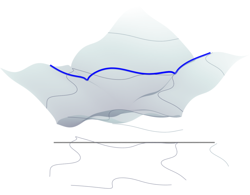
The remainder of the paper is divided in two parts corresponding to the prototype functionals (2) and (3). These are rather different, and to explain why note that $\mathcal{S}(f)$ can be computed explicitly only if the global minimum of the original functional (5) can be found explicitly, as in the case of (3) but not (2). Therefore, the problem of minimizing (3) only becomes difficult in combination with additional restrictions. Suppose e.g. that we want to minimize (5) over some subspace $\mathcal{M}\subset\mathcal{V}$ or say that we wish to minimize $f(x)+\frac{1}{2}\|x-d\|^{2}+c(x)$ where $c$ is a convex functional related to any additional prior information, (see Section 4 in [32] for concrete examples). In both cases we end up with minimization problems with no closed form solution. Replacing $f$ with $\mathcal{S}^{2}(f)$ then gives us a convex problem, similar to the original one, which can be addressed with standard convex approximation schemes like the projected subgradient method, dual ascent, ADMM or forward-backward splitting. It is often the case that the minimum of the “convexified” problem coincides with the minimum of the non-convex problem, which is easily verified by simply checking if $f(x)=\mathcal{S}^{2}(f)(x)$ holds at the point of convergence. It is important however to realize that this is not always the case, as Figure 2 demonstrates. However, Figure 6 in Section 3.1 shows the same functional with a different subspace on which the two minima does coincide. We elaborate further on this in Section 3.1. It is not the aim of the present paper to provide recommendations for which algorithm to use to solve a specific application, and the best candidate will certainly depend on the particular situation. Nevertheless, several of the algorithms mentioned above requires the ability to compute the so called proximal operator, and we provide theory for this in Section 3.2, which concludes Part II of the paper, titled “applications with additional priors”.

Part III of the paper is devoted to the problem of minimizing

where $A$ is any linear transformation. We assume that $\mathcal{V}$ is such that $\mathcal{S}^{2}_{\gamma}(f)$ is computable, but due to the linear transformation $A$, the functional

will not equal the convex envelope of (7), which we assume is untractable, as in the case of (2). The parameter $\gamma$ now becomes a valuable tool as it tunes the curvature of $\mathcal{S}_{\gamma}^{2}(f)$. The expression (8) is illustrated (in one dimension and for values of $|A|^{2}>\gamma$ (left) and $|A|^{2}<\gamma$ (right)) in Figure 3. The circles represent global minima of the respective functions.

Generalizing the left figure, we assume in Section 4.2 that $\gamma$ is below the square of the lowest singular value of $A$. We prove that the functional (8) is a convex functional below (7), and hence minimization of (8) will produce a minimizer which, although not necessarily equal to the minimizer of the original problem, likely is closer than that obtained by other convex relaxation methods (if such at all are available). Moreover, the minimizer of the original and modified problem do coincide whenever $f(x)=\mathcal{S}_{\gamma}^{2}(f)(x)$, which often is easily checked in practice. An example of when this happens, similar to Figure 3, is shown in Figure 7 in Section 4.2.

For the problem (2), $A$ is usually a matrix with a large kernel, and the smallest singular value is 0, which rules out the above approach. In Section 4.3 we consider the case $\gamma>\|A\|^{2}$, generalizing the situation in the right picture of Figure 3. We can then show that (8) is a continuous (but not everywhere convex) functional with the following desirable properties; $i)$ (8) lies between (7) and its l.s.c. convex envelope, $ii)$ any local minimizer of (8) is a local minimizer of (7), $iii)$ the global minimizers of (8) and (7) coincide (see Proposition 4.5 and Theorem 4.6). We remark that, despite not being convex, critical points of (8) can be found using e.g. the forward-backward splitting method [7, 12]. The situation in Section 4.3 is thus drastically different from the previous scenarios; whether a global minimizer of the original problem is found depends only on the starting point for the algorithm seeking local minimizer. This latter part of the paper is inspired by [48], which considers problem (2), and also contains a list of recent algorithms for finding local minima of functionals of the type considered above. A separate study of the methods developed here to this particular problem is also found in our recent contribution [19].

The set of $m\times n$ complex matrices, equipped with the Frobenius norm, is denoted $\mathbb{M}_{m,n}$. Throughout the paper, $\mathcal{V}$ and sometimes $\mathcal{W}$ denote separable Hilbert spaces (possibly finite dimensional). Let $\mathcal{B}_{2}(\mathcal{V},\mathcal{W})$ denote all Hilbert-Schmidt operators with the Hilbert-Schmidt norm. We remark that in case $\mathcal{V}=\mathbb{C}^{n}$ and $\mathcal{W}=\mathbb{C}^{m}$ with the canonical norms, then $\mathcal{B}_{2}(\mathcal{V},\mathcal{W})$ is readily identified with $\mathbb{M}_{m,n}$ with the Frobenius norm. The singular value decomposition (SVD) of a given $A\in\mathbb{M}_{m,n}$ is denoted $A=U\Sigma V^{*}$, where we choose $V\in\mathbb{M}_{n,n}$, $\Sigma\in\mathbb{M}_{n,n}$ and $U\in\mathbb{M}_{m,n}$. The vector of singular values (i.e. the elements on the diagonal of $\Sigma$) is then denoted by $\sigma.$ Note that we thus define the singular values such that the amount of singular values equals the dimension of $\mathcal{V}$. More generally, given any operator $A$ acting on infinite dimensional spaces, we can pick singular vectors $(u_{j})_{j=1}^{\infty}$ and $(v_{j})_{j=1}^{\infty}$ such that

where $\sigma_{j}(A)$ are the singular values (ordered decreasingly) and $u_{j}\otimes v_{j}(x)=u_{j}\left\langle x,v_{j}\right\rangle$. Moreover $(u_{j})_{j=1}^{\infty}$ can be taken to be an orthonormal sequence in $\mathcal{W}$ and $(v_{j})_{j=1}^{\infty}$ to be an orthonormal basis in $\mathcal{V}$ (see e.g. Theorem 1.4 [47]). We follow the matrix theory custom of numbering the singular vectors starting at 1, as opposed to 0 which is more common in operator theory.

$\mathbb{H}(\mathcal{V})$ will denote the subspace of ${\mathcal{B}}_{2}(\mathcal{V},\mathcal{V})$ of self-adjoint (Hermitian) operators, and $\lambda(X)$ the vector of eigenvalues of a given $X\in\mathbb{H}(\mathcal{V})$. In case $\mathcal{V}$ has finite dimension $n$, so that ${\mathcal{B}}_{2}(\mathcal{V},\mathcal{V})$ is identified with $\mathbb{M}_{n,n}$, we simply write $\mathbb{H}_{n}$.

$\mathbb{R}^{d}$ for $d=\infty$ is identified with $\ell^{2}(\mathbb{N})$. Given $x\in\mathbb{R}^{d}$, $\|x\|_{0}$ denotes the amount of non-zero elements (by abuse of notation since this is not a norm), and $\|x\|_{2}$ the canonical norm. We abbreviate lower semi-continuous by l.s.c., and we denote by $\mathsf{dom}(f)$ the set of points where the functional $f$ is finite. Both $CE(f)$ and $f^{**}$ will denote the l.s.c convex envelope of a functional $f$.

$\mathcal{S}_{\mathcal{V},\gamma}$ is the $\mathcal{S}$-transform computed with the scalar product of $\mathcal{V}$ and parameter $\gamma$. Usually $\mathcal{V}$ is omitted from the notation and furthermore when $\gamma=1$ we simply write $\mathcal{S}$.

References

- [1] Fredrik Andersson and Marcus Carlsson. Alternating projections on nontangential manifolds. Constructive Approximation, 38(3):489–525, 2013.
- [2] Fredrik Andersson and Marcus Carlsson. On the structure of positive semi-definite finite rank general domain hankel and toeplitz operators in several variables. Complex Analysis and Operator Theory, pages 1–30, 2016.
- [3] Fredrik Andersson and Marcus Carlsson. Fixed-point algorithms for frequency estimation and structured low rank approximation. Applied and Computational Harmonic Analysis, 2017.
- [4] Fredrik Andersson, Marcus Carlsson, and Herwig Wendt. On a fixed-point algorithm for structured low-rank approximation and estimation of half-life parameters. In Signal Processing Conference (EUSIPCO), 2016 24th European, pages 326–330. IEEE, 2016.
- [5] Fredrik Andersson, Marcus Carlsson, and Carl Olsson. Convex envelopes for fixed rank approximation. Optimization Letters, 11(8):1783–1795, 2017.
- [6] H Attouch and D Azé. Approximation and regularization of arbitrary functions in hilbert spaces by the lasry-lions method. In Annales de l’IHP Analyse non linéaire, volume 10, pages 289–312, 1993.
- [7] Hedy Attouch, Jérôme Bolte, and Benar Fux Svaiter. Convergence of descent methods for semi-algebraic and tame problems: proximal algorithms, forward–backward splitting, and regularized gauss–seidel methods. Mathematical Programming, 137(1-2):91–129, 2013.
- [8] Heinz H Bauschke and Patrick L Combettes. Convex analysis and monotone operator theory in Hilbert spaces. Springer Science & Business Media, 2011.
- [9] Heinz H Bauschke, Rafal Goebel, Yves Lucet, and Xianfu Wang. The proximal average: basic theory. SIAM Journal on Optimization, 19(2):766–785, 2008.
- [10] Amir Beck. On the convergence of alternating minimization for convex programming with applications to iteratively reweighted least squares and decomposition schemes. SIAM Journal on Optimization, 25(1):185–209, 2015.
- [11] Jacek Bochnak, Michel Coste, and Marie-Françoise Roy. Real algebraic geometry, volume 36. Springer Science & Business Media, 2013.
- [12] Jérôme Bolte, Shoham Sabach, and Marc Teboulle. Proximal alternating linearized minimization for nonconvex and nonsmooth problems. Mathematical Programming, 146(1-2):459–494, 2014.
- [13] Jonathan M Borwein and Chris H Hamilton. Symbolic fenchel conjugation. Mathematical Programming, 116(1-2):17–35, 2009.
- [14] Bernard Brighi and Michel Chipot. Approximated convex envelope of a function. SIAM journal on numerical analysis, 31(1):128–148, 1994.
- [15] Arne Brø ndsted. Milman’s theorem for convex functions. Mathematica Scandinavica, 19:5–10, 1966.
- [16] James A Cadzow. Signal enhancement-a composite property mapping algorithm. IEEE Transactions on Acoustics, Speech, and Signal Processing, 36(1):49–62, 1988.
- [17] Emmanuel J Candès, Justin Romberg, and Terence Tao. Robust uncertainty principles: Exact signal reconstruction from highly incomplete frequency information. Information Theory, IEEE Transactions on, 52(2):489–509, 2006.
- [18] Marcus Carlsson. On convex envelopes and regularization of non-convex functionals without moving global minima. arXiv preprint https://arxiv.org/abs/1811.03439, 2018.
- [19] Marcus Carlsson, Daniele Gerosa, and Carl Olsson. A un-biased approach to compressed sensing. arXiv preprint https://arxiv.org/abs/1806.05283, 2018.
- [20] Patrick L Combettes and Valérie R Wajs. Signal recovery by proximal forward-backward splitting. Multiscale Modeling & Simulation, 4(4):1168–1200, 2005.
- [21] John B Conway. A course in operator theory. American Mathematical Soc., 2000.
- [22] John B Conway. A course in functional analysis, volume 96. Springer Science & Business Media, 2013.
- [23] Eduardo Marques de Sá. Exposed faces and duality for symmetric and unitarily invariant norms. Linear Algebra and its Applications, 197:429–450, 1994.
- [24] David L Donoho. For most large underdetermined systems of linear equations the minimal -norm solution is also the sparsest solution. Communications on pure and applied mathematics, 59(6):797–829, 2006.
- [25] Henry R Dowson. Spectral theory of linear operators, volume 12. Academic Pr, 1978.
- [26] Nelson Dunford and Jacob T Schwartz. Linear operators. Part 2: Spectral theory. Self adjoint operators in Hilbert space. Interscience Publishers, 1963.
- [27] Jonathan Gillard and Anatoly Zhigljavsky. Optimization challenges in the structured low rank approximation problem. Journal of Global Optimization, 57(3):733–751, 2013.
- [28] Pinghua Gong, Changshui Zhang, Zhaosong Lu, Jianhua Huang, and Jieping Ye. A general iterative shrinkage and thresholding algorithm for non-convex regularized optimization problems. In ICML (2), pages 37–45, 2013.
- [29] Markus Grasmair. Non-convex sparse regularisation. Journal of Mathematical Analysis and Applications, 365(1):19–28, 2010.
- [30] Waren L Hare. A proximal average for nonconvex functions: a proximal stability perspective. SIAM Journal on Optimization, 20(2):650–666, 2009.
- [31] Warren Hare and Claudia Sagastizábal. Computing proximal points of nonconvex functions. Mathematical Programming, 116(1-2):221–258, 2009.
- [32] Viktor Larsson and Carl Olsson. Convex low rank approximation. International Journal of Computer Vision, pages 1–21, 2016.
- [33] Jean-Michel Lasry and Pierre-Louis Lions. A remark on regularization in hilbert spaces. Israel Journal of Mathematics, 55(3):257–266, 1986.
- [34] Adrian S Lewis and Jérôme Malick. Alternating projections on manifolds. Mathematics of Operations Research, 33(1):216–234, 2008.
- [35] Yves Lucet. The Legendre-Fenchel Transform and the Convex Hull of a Function: Fast Computational Algorithms, Second-Order Smoothness and Analysis. PhD-thesis; https://people.ok.ubc.ca/ylucet/thesis/1997-PhD Yves lucet.pdf, 1997.
- [36] Yves Lucet. What shape is your conjugate? a survey of computational convex analysis and its applications. SIAM review, 52(3):505–542, 2010.
- [37] Garth P McCormick. Computability of global solutions to factorable nonconvex programs: Part i—convex underestimating problems. Mathematical programming, 10(1):147–175, 1976.
- [38] Clifford A Meyer and Christodoulos A Floudas. Convex envelopes for edge-concave functions. Mathematical programming, 103(2):207–224, 2005.
- [39] Peter Ochs, Alexey Dosovitskiy, Thomas Brox, and Thomas Pock. On iteratively reweighted algorithms for nonsmooth nonconvex optimization in computer vision. SIAM Journal on Imaging Sciences, 8(1):331–372, 2015.
- [40] Neal Parikh and Stephen P Boyd. Proximal algorithms. Foundations and Trends in optimization, 1(3):127–239, 2014.
- [41] Benjamin Recht, Maryam Fazel, and Pablo A. Parrilo. Guaranteed minimum-rank solutions of linear matrix equations via nuclear norm minimization. SIAM Rev., 52(3):471–501, August 2010.
- [42] John R Ringrose. Compact non-self-adjoint operators. von Nostrand, 1971.
- [43] R Tyrrell Rockafellar and Roger J-B Wets. Variational analysis, volume 317. Springer Science & Business Media, 2009.
- [44] Rayan Saab and Özgür Yılmaz. Sparse recovery by non-convex optimization–instance optimality. Applied and Computational Harmonic Analysis, 29(1):30–48, 2010.
- [45] Robert Schatten. Norm ideals of completely continuous operators, volume 27. Springer-Verlag, 1960 (2013).
- [46] Ivan Selesnick. Sparse regularization via convex analysis. Transactions, 1, 2017.
- [47] Barry Simon. Trace ideals and their applications, volume 35. Cambridge University Press Cambridge, 1979.
- [48] Emmanuel Soubies, Laure Blanc-Féraud, and Gilles Aubert. A continuous exact ell_0 penalty (cel0) for least squares regularized problem. SIAM Journal on Imaging Sciences, 8(3):1607–1639, 2015.
- [49] Thomas Strömberg. On regularization in banach spaces. Arkiv för Matematik, 34(2):383–406, 1996.
- [50] Paul Tseng. Approximation accuracy, gradient methods, and error bound for structured convex optimization. Mathematical Programming, 125(2):263–295, 2010.
- [51] Yaoliang Yu, Xun Zheng, Micol Marchetti-Bowick, and Eric P Xing. Minimizing nonconvex non-separable functions. In AISTATS, 2015.