Shock-driven Accretion in Circumplanetary Disks: Observables and Satellite Formation
Abstract
Circumplanetary disks (CPDs) control the growth of planets, supply material for satellites to form, and provide observational signatures of young forming planets. We have carried out two dimensional hydrodynamical simulations with radiative cooling to study CPDs, and suggested a new mechanism to drive the disk accretion. Two spiral shocks are present in CPDs, excited by the central star. We find that spiral shocks can at least contribute to, if not dominate the angular momentum transport and energy dissipation in CPDs. Meanwhile, dissipation and heating by spiral shocks have a positive feedback on shock-driven accretion itself. As the disk is heated up by spiral shocks, the shocks become more open, leading to more efficient angular momentum transport. This shock driven accretion is, on the other hand, unsteady on a timescale of months/years due to production and destruction of vortices in disks. After being averaged over time, a quasi-steady accretion is reached from the planet’s Hill radius all the way to the planet surface, and the disk -coefficient characterizing angular momentum transport due to spiral shocks is 0.001-0.02. The disk surface density ranges from 10 to 1000 g cm-2 in our simulations, which is at least 3 orders of magnitude smaller than the “minimum mass sub-nebula” model used to study satellite formation; instead it is more consistent with the “gas-starved” satellite formation model. Finally, we calculate the millimeter flux emitted by CPDs at ALMA and EVLA wavelength bands and predict the flux for several recently discovered CPD candidates, which suggests that ALMA is capable of discovering these accreting CPDs.
Subject headings
hydrodynamics, accretion, accretion disks, planets and satellites: detection, planets and satellites: formation, planet-disk interactions, shock wavesI. Introduction
Planets form and grow in circumstellar disks. Initally when a protoplanet forms, the solid core is surrounded by a hydrostatic gaseous envelope that is in contact with the planet’s Hill sphere and the rest of the circumstellar disk. As the core’s mass increases, the planet envelope contracts due to both the stronger gravity and cooling through radiation. Eventually, when the core mass reaches , the planet undergoes runaway accretion and contracts significantly. At this stage, the envelop shrinks significantly and detaches from the planet’s Hill sphere (Papaloizou & Nelson 2005). Material that resides beyond the Hill sphere can still flow into the Hill sphere, but forms a circumplanetary disk (CPD) around the protoplanet to conserve angular momentum (Lubow et al. 1999; Ayliffe & Bate 2009). The accretion of the circumplanetary disk (CPD) onto the planet allows the continuous growth of the planet even after the planet’s runaway growth stage.
Circumplanetary disks (CPDs) may provide observational signatures of young forming planets in disks. Giant planets can be too faint to be detected, but accreting CPDs can be bright and detectable. For example, to form a giant planet of 110 MJ mass within the circumstellar disk’s life time ( a few million years, Hernandez et al. 2007), the CPD needs to accrete at a rate of . Such an accretion disk will have a luminosity (e.g. Owen 2014, Zhu 2015) of
| (1) |
which is as bright as a late M-type/early L-type brown dwarf and can be detected by current direct imaging techniques (Zhu 2015). Unlike a planet or brown dwarf which has an almost constant surface temperature, an accreting CPD has a lower temperature at larger disk radii, and those outer disk regions will emit significant infrared flux. Thus, the emission from an accreting CPD is redder than the emission from a planet or a brown dwarf. Direct imaging observations have found several red sources within circumstellar disks (Kraus & Ireland 2012, Quanz et al. 2013, Biller et al. 2014, Reggiani et al. 2014, Currie et al. 2015) and their photometry at near-IR bands are consistent with accreting CPDs (Zhu et al. 2015). emission lines, which are another observational signature of accretion disks, are also found in some low-mass substellar objects (Zhou et al. 2014, Bowler et al. 2015). The most direct evidence for accreting CPDs is LkCa 15b, where two accretion tracers, Hα line and near-IR thermal emission, have both been detected (Sallum et al. 2015).
CPDs are also essential for satellite formation. In our solar system, most satellites around giant planets are in prograde, nearly circular and coplanar orbits, implying that they formed in a shared CPD orbiting within the planet’s equatorial plane. The ratio between the total mass of four major Galilean satellites and the Jupiter’s mass is . The Saturnian satellite system also has a similar mass fraction with respect to the Saturn’s mass (Canup & Ward 2006). Assuming the gas-to-dust mass ratio is 100, a minimum gas mass of planet mass is required to produce these satellites (Canup & Ward 2002, 2006). There are two main scenarios for Galilean satellite formations. One assumes that the satellites form in-situ in a CPD containing this amount of material (e.g. Lunine & Stevenson 1982; Mosqueira & Estrada 2003). This disk is referred to as the “minimum mass sub-nebula”, which is the analog of “minimum mass nebula” for the circumstellar disk. Spreading 0.02 Jupiter mass within 30 Jupiter radii (where the four major satellites reside), the minimum mass sub-nebula has a very high gas surface density . In the other scenario, the satellites form in a CPD with a much lower surface density, but the disk is dynamically evolving and being supplied by the circumstellar disk (Canup & Ward 2002, 2006). This “gas-starved” scenario only requires that the total supplied mass during the whole satellite formation timescale is larger than planet mass.
The key question for understanding the structure of CPDs is how CPDs accrete. They may accrete in similar ways as circumstellar disks accrete. Turner et al. (2014) suggest that the surface of CPDs can be ionized by X-rays so that the magnetorotational instability (MRI) can operate at the disk surface leading to accretion, a process similar to the layered accretion proposed in protoplanetary disks (Gammie 1996). However, Fujii et al. (2011, 2014) find that the active layer is so thin () in CPDs that the accretion through MRI is negligible. On the other hand, other non-ideal MHD effects (e.g. Hall effects, Kunz & Lesur 2013, Lesur et al. 2014, Bai 2014) which are important in protoplanetary disks can also be important in CPDs, and CPDs may accrete through magnetic breaking (Keith & Wardle 2014). Magnetocentrifugal disk wind can also be launched in CPDs, carrying away angular momentum and leading to disk accretion (Quillen & Trilling 1998, Gressel et al. 2013). Almost all these proposed CPD accretion mechanisms (e.g. layered accretion, non-ideal MHD effects, disk wind) can find their roots in circumstellar disk models. Thus, they are facing the same uncertainties as the accretion mechanisms in circumstellar disks: they sensitively depend on the net magnetic fields assumed and the detailed microphysics in the disk (e.g. dust size distribution).
On the other hand, CPDs are different from circumstellar disks in that they are subject to the tidal torque from the central star, and truncated within the Hill sphere of the planet (Martin & Lubow 2011a). In addition, circumstellar disk material flows through the Hill sphere, continuously replenishing CPDs. These properties make CPDs similar to disks with inflows from companion stars in close binary systems or Cataclysmic Variables (CV). In these binary systems, the tidal torque from the companion star will excite spiral density waves in disks, and when these waves shock in disks, they can transport angular momentum to the disk leading to disk accretion. Previous inviscid isothermal simulations by Rivier et al. (2012) have suggested that accretion due to spiral shocks in CPDs is inefficient with Jupiter’s mass doubling time 5 Myrs. Szulágyi et al. (2014) have measured a much higher accretion rate in their 3-D isothermal inviscid simulations (10-4 MJ/yr), but this measured accretion rate is not numerically converged with their higher resolution simulations. Instead, by measuring the torque exerted by the star in the simulations, they estimate that the real accretion rate is MJ/yr.
Recent studies on spiral shocks (Ju et al. 2016) have shown that the accretion due to spiral shock dissipation is sensitive to the disk thermodynamics assumed. When the disk is hot and the Mach number, defined as the ratio between the Keplerian speed and the sound speed, is small (10), the equivalent of shock-driven accretion can reach 0.01-0.02. The Mach number of CPDs depends on the disk accretion rate and is sensitive to the equation of state applied in simulations (D’Angelo et al. 2003, Ayliffe & Bate 2009, Machida 2009, Szulágyi et al. 2016).
Considering the potential importance of spiral shocks driving accretion in CPDs, in this paper we construct two-dimensional inviscid hydrodynamical simulations to study CPDs. These inviscid simulations differ from most previous works that use artificial viscosity (e.g. viscosity) to sustain the disk accretion. Furthermore, to reduce the numerical viscosity in the CPD region, we adopt a grid structure centered on the planet. Since the thermodynamics which controls the disk Mach number is crucial for the shock-driven accretion, a simple radiative cooling scheme has been included in the simulations, which differs this work from inviscid simulations by Rivier et al. (2012) and Szulágyi et al. (2014). We have also measured the mass accretion rate directly from simulations, unlike these two works where they use the torque exerted by the star onto the CPD to estimate the disk accretion rate. As Ju et al. (2016) has pointed out, shock-driven accretion is determined by the shock dissipation (the difference between the tidal torque exerted to the disk and the angular momentum flux carried away by the wave), instead of the total torque alone. We will show that, by allowing the disk being heated up by the shock, the inviscid simulation is numerically converged and the disk can reach a steady state, transferring inflow material from the Hill radius all the way to the central planet quasi-steadily. This shock driven accretion is very efficient with .
One caveat in our simulations is that our simulations are limited to 2-D and numerous previous 3-D simulations have shown that the infall from circumstellar to circumplanetary disks occurs at high altitudes (Bate et al. 2003, Machida et al. 2008, Tanigawa et al. 2012, Morbidelli et al. 2014, Szulágyi et al. 2014, 2016). Furthermore, since the CPD is significantly heated and puffed up, our simple cooling treatment based on the thin disk approximation is inaccurate. 3-D simulations with realistic radiative transfer (Szulágyi et al. 2016), thermodynamics, planet evolution (Ward & Canup 2010) and even planetesimal accretion (D’Angelo & Podolak 2015) are needed in future to confirm if spiral shocks can lead to efficient accretion in CPDs.
In §2, our numerical method is introduced. The results are presented in §3, including both the disk structure and the accretion rate. After a short discussion in §4, the paper will be concluded in §5. The detailed energy budget of the accretion process is given in the appendix.
II. Method
We solve the Euler equations to study dynamics in CPDs using Athena++ (Stone et al. 2016, in preparation). Athena++ is a newly developed grid based code using a higher-order Godunov scheme for MHD and the constrained transport (CT) to conserve the divergence-free property for magnetic fields. Compared with its predecessor Athena (Gardiner & Stone 2005, 2008; Stone et al. 2008), Athena++ is highly optimized for speed and uses flexible grid structures, allowing global numerical simulations spanning a large radial range. Furthermore, the geometric source terms in curvilinear coordinates (e.g. in cylindrical and spherical-polar coordinates) are carefully implemented so that angular momentum is conserved exactly (to machine precision), which is crucial for angular momentum budget analysis in §3.2.
In this paper, magnetic fields are ignored. We solve hydrodynamical equations in the cylindrical coordinate system ( and ) that is centered on the planet. This grid choice is different from most previous works which have adopted cylindrical or spherical coordinate systems that are centered on the star. Having the cylindrical coordinate system centered on the planet allows the material in CPDs flow along the azimuthal grid direction, thus significantly reduces numerical truncation errors. Adopting the cylindrical coordinate system with uniform grids in ln() also allows each grid to have the same length along the azimuthal and radial direction throughout the whole simulation domain .
Furthermore, we adopt the rotating frame so that the star is stationary at =1, =0. The equations being solved are
| (2) | ||||
| (3) | ||||
| (4) |
where is the disk surface density, is the linear momentum, =-GMp/R is the potential of the planet having the mass of Mp, and is the total energy density per unit area with being the internal energy. Note that since the planet is at the coordinate center, coordinate and are the position relative to the planet instead of the star. is the total external force excluding the gravitational force from the planet, and thus includes the centrifugal force and Coriolis force due to the adoption of the rotating frame, the direct gravitational force from the star, and the indirect force (since the grid is centered at the planet instead of the center of mass). The detailed forms of these terms are given in Ju et al. (2016). Solving these equations in cylindrical coordinates also introduces geometrical source terms, which are written in forms of conserving the angular momentum with machine error precision (as in Ju et al. 2016). As will be shown in §3.2, maintaining angular momentum conservation is crucial for the angular momentum diagnostics.
No physical viscosity has been applied in our simulations. Thus, angular momentum and energy transport can only come from shock dissipation and numerical viscosity. Since simulations having twice resolution produce almost identical results, which will be shown below, we conclude that numerical viscosity is negligible and angular momentum and energy transport is dominated by the shock dissipation.
The equation of state for an ideal gas has been assumed, so that . We further assume =7/5. The density-weighted disk temperature is , where is the gas constant and . Since most disk mass is concentrated at the disk midplane, we use to approximate the disk midplane temperature .
The cooling rate per unit area, , is approximated by
| (5) |
where is the optical depth to the disk midplane at radius (Hubeny 1990). The midplane density is where is the disk scale height . The Rosseland mean opacity is assumed to be 10 , which is the typical value (D’Alessio et al. 2001) at temperatures below the dust sublimation temperature of 1500 K 11 1 In some of the runs, the temperature of the very inner disk goes above the dust sublimation temperature and the opacity should decrease dramatically. However, we still use a constant opacity to avoid disk instability associated with the opacity change (Zhu et al. 2009). . The particular form is chosen so that the cooling term has the correct form in both optically thick and thin limits 22 2 In the optically thin limit, we should use the Planck mean opacity. Because the dominant opacity is from dust, which has a relatively slow variation with wavelength, we use the Rosseland mean opacity for simplicity.. The term represents the energy flux into the disk from the stellar irradiation, leading to a background disk temperature of .
Due to the inclusion of the thermodynamics in the problem, we have to specify physical units in the simulations. We assume that the distance between the star and the planet is 5 AU, the star is a solar mass star, and the planet’s mass is 0.001 (). is 128 K so that the aspect ratio of the circumstellar disk at the planet position ( where is Jupiter’s orbital velocity around the Sun) is 0.05. Besides the simulations with radiative cooling, we have also carried out simulations with isothermal and adiabatic equations of state for comparison.

Our cylindrical grids are uniformly spaced from to in the direction, and uniformly spaced in ln() from 2 or 4 Jupiter radii to half the distance between the planet and the star (which is 2.5 AU). Given an adopted resolution in the radial direction, we adjust the resolution in the azimuthal direction to make sure every grid cell is square in physical size. Since a Jupiter mass planet should induce a gaseous gap in the circumstellar disk (Lin & Papaloizou 1986, Kley & Nelson 2012), we have manually carved out a gap in the simulations as shown in Figure 1. Motivated by detailed gap opening studies (e.g. de Val-Borro et al. 2006, Fung et al. 2014), we parameterize the gap density profile as
| (6) |
where and are the disk surface density within and outside the gap, is the gap half width, represents the sharpness of the gap, and represents how far away each point is from the gap center, and is the star’s position in the planet centered frame. In all our simulations, we choose AU, which is roughly 1/6 to 1/4 of the gap half width. The velocity field is initialized by maintaining hydrostatic equilibrium in the radial direction by balancing the pressure gradient, the central stellar gravity, centrifugal and Coriolis forces. We have tested that the gap shape is nicely maintained in the simulation where there is no planet at the center. We also initialize a Keplerian CPD with a very low surface density ( g cm-2) within 0.4 Jupiter’s Hill radii.
To maintain the gap structure during the simulation, we fix physical quantities at the outer boundary to be the initial values. At the inner boundary, we adopt the “outflow, no inflow” open boundary condition. The density and radial velocity are copied from the last active zones to the ghost zones. When the radial velocity is towards the computational domain, it is set to be zero. The azimuthal velocity in the ghost zones are set to their local Keplerian values. Internal energy in the ghost zones is the same as that in the last active zones.
Our initial and boundary condition are quite different from those used in previous circumplanetary disk simulations. Instead of capturing the planet gap opening process in the simulation, we prescribe the gap density profile based on detailed gap opening studies (e.g. de Val-Borro et al. 2006, Fung et al. 2014). By this approach, the gap shape is fixed and the inflow from the circumstellar disk to the circumplanetary disk can reach a steady state. In reality, the detailed gap width and depth depend on the disk turbulent level, the disk thermal structure and even the magnetic field geometry (Zhu et al. 2013). In inviscid disks, the gap will even become deeper with time (Zhu et al. 2013). To simplify the gap opening process, we use different gap widths and depths in different simulations, to represent the gaps in disks with different properties or during different stages of the gap opening process. We also use these different gap widths and depths to control the inflow rate to the CPD. In our simulations, we allow the circumplanetary region to settle down by itself and have no direct control of the inflow rate to the CPD. Thus, we take advantage of the fact that the simulation with a wider and deeper gap has a lower inflow rate to the CPD, and, through varying gap shapes, we indirectly control the inflow rate to cover 4 orders of magnitude.
| Run | EoS | Resolution | Time | |||
|---|---|---|---|---|---|---|
| g cm-2 | g cm-2 | yr | ||||
| Gp2 | Cool | 432352 | 10 | 0.1 | 1 | 210 |
| Gp2H | Cool | 864704 | 10 | 0.1 | 1 | 85 |
| Gp2adi | Adi. | 432352 | 10 | 0.1 | 1 | 250 |
| Gp3 | Cool | 432352 | 10 | 0.1 | 1.5 | 250 |
| Gp3iso | Iso. | 432352 | 10 | 0.1 | 1.5 | 297 |
| Gp3Sp1 | Cool | 432352 | 1 | 0.01 | 1.5 | 515 |
| Gp3Sp01a | Cool | 400352 | 0.1 | 10-3 | 1.5 | 1216 |
| Gp3Sp001a | Cool | 400352 | 0.01 | 10-4 | 1.5 | 2485 |
All simulations are summarized in Table 1. The number after the capital letter “G” (where p2 means 0.2) represents the gap half width () in the code unit (1 is 5 AU). The number after the capital letter S represents the circumstellar disk surface density () relative to the surface density in the fiducial case (Gp2). Our fiducial case (Gp2) has a circumstellar disk with 10 g cm-2 surface density, which is one order of magnitude smaller than the surface density at 5 AU based on the minimum mass solar nebula model (Hayashi et al. 1981). The simulations having “iso” and “adi” in their names are isothermal and adiabatic simulations. All other simulations have considered simple radiative cooling (Equation 5). For simulations with low circumstellar surface density and thus low inflow rates (Gp3Sp01 and Gp3Sp001), the CPDs take much longer to a reach steady state. Thus, we have to adopt a bigger inner boundary (4 Jupiter radii) to speed up the calculations and a higher initial CPD surface density to reduce the time to reach a steady state.
III. Results
The typical disk surface density during the simulation is shown in Figure 1. The morphology of CPD is very similar to previous studies (e.g. Lubow et al. 1999). Gas material in the circumstellar disk enters the Roche sphere of the planet when the gas undergoes horseshoe orbits around the planet. The planet excites spiral arms in the circumstellar disk, while the star excites spiral arms in the CPD. These spiral arms in CPDs are crucial for angular momentum transport in CPDs as shown in §3.2.
III.1. Disk Structure


We have run these simulations until they reach quasi-steady state, except for the isothermal case which shows no sign of reaching a steady state during the whole run 33 3 After a long simulation time, the isothermal case may eventually reach a steady state when enough material is piled up in the CPD. . The total mass of the CPD within the Hill sphere (0.347 AU) is shown in Figure 2. When a quasi-steady state has been reached, the accretion rate onto the planet equals the inflow rate, and the disk mass remains a constant. Disks with narrower (smaller ) gaps and higher surface density (higher and ) have higher inflow rate from the circumstellar disk to the CPD. For case Gp2 which has the highest accretion rate, the CPD reaches a steady state within 50 years. For cases with low accretion rates (e.g. Gp3Sp001), the disk reaches a quasi-steady state on the timescale of 1000 years. For a comparison with the dynamical timescale, the orbital time at our inner boundary (2 RJ) and half the Hill radii is only 8 hours and 2.3 years respectively. Thus, 100 years which is the typical duration of the simulation is 1.1 innermost orbits.


The accretion onto the planet is not strictly steady with time. As shown in Figures 2-4 and also in Ju et al. (2016), there are short timescale variabilities. The disk accretion rates at the inner boundary and at =10 are shown in the upper left panels of Figure 3 and 4 for both Gp2 and Gp3Sp001 respectively. The accretion rates in these panels have been averaged over 1 . For case Gp2, there is significant variability even within the timescale of 1 . Thus, we plot the accretion rates at a much higher cadence (averaged over 0.01 ) within a short period of time. To understand the short-timescale variability, we plot the disk surface density profile at different times during the outburst, as shown in the upper right panels of Figure 3 and 4. The 2-D surface density contours at these two times are shown in the lower left two panels of these figures (the lower left panel corresponds to the black curve in the upper right panel, while the lower middle panel corresponds to the red curve.). We can see that the disk develops significant asymmetric structure during these accretion peaks. Vortices are generated in these disks first. As clearly shown in Figure 4, banded structures are first induced by spiral shocks, and these structures are subject to Rossby Wave Instability (Lovelace et al. 1999) and become vortices. In the lower left panel of Figure 3, a vortex forms at the outer disk and migrates inwards. Eventually it crosses the inner boundary (lower middle panel), leading to an outburst. In Figure 4, the vortex does not migrate significantly in the disk, but it excites spiral arms, leading to additional angular momentum transport.
Thus, vortices provide some other ways to transport angular momentum in the disk, which are different from the accretion process due to star-induced spiral shocks mentioned above. First, vortices can excite spiral density waves, which can become spiral shocks and transport angular momentum. Secondly, vortices themselves will migrate in disks (Paardekooper et al. 2010), and this vortex migration directly leads to mass transport since the vortex region has a high disk surface density. Thus, it is important to know how much disk accretion is driven by star-induced spiral shocks and how much accretion is due to vortices generated. Unfortunately, using Reynolds stress alone, as in §3.2, we cannot distinguish these accretion mechanisms. On the other hand, we can use the change of the Reynolds stress when a vortex appears or disappears in the disk to qualitatively study the role played by the vortex. As shown in the bottom right panels of Figures 3 and 4, the Reynolds stress does not change significantly when there is a vortex in the disk. This suggests that the spiral shocks play a more important, if not dominate, role in transporting angular momentum in disks.
On the other hand, vortices regulate the disk accretion rate, causing episodic accretion. And, for the disks with higher accretion rates, vortices are generated at smaller radii (by comparing Figure 3 and 4), leading to shorter timescale and more violent outbursts.

To remove the short-timescale variability and study the general properties of disk structure, we average the mass accretion rate and surface density at each time step over 10 (18 years, for the high resolution case, Gp2H), 50 (90 years, for fiducial resolution cases with 2 RJ inner boundary), or 100 (180 years, for fiducial resolution cases with 4 RJ inner boundary) before the end of the simulations, and plot the azimuthally averaged values in Figure 5. For reference, the Hill radius is 740 RJ. The time-averaged disk accretion rates in our models span a large range from 10-9 MJ/yr to 10-5 MJ/yr (the upper left panel). In all the cases except the isothermal case, the accretion rate is almost a constant throughout the whole disk, implying that the disk reaches a quasi-steady state. In the isothermal case, the disk has a low temperature and the spiral shocks are so tightly wound up at the inner disk and spiral shocks are inefficient to carry away angular momentum there (Ju et al. 2016, also in §3.2). Among all the models with radiative cooling, the disk surface density only spans one order of magnitude despite the large range of disk accretion rates. The maximum surface density is between 50 g cm-2 and 500 g cm-2 in these models (the upper right panel).
The disk midplane temperature and aspect ratio at the end of the simulations are shown in the bottom panels of Figure 5. The aspect ratio of the CPD is defined similarly as the aspect ratio of the circumstellar disk. It is the ratio between the disk scale height (H) and the radius (R) in the CPD, which is equal to with being the orbital velocity around the planet. The disk midplane temperature varies significantly among cases. In simulations that have realistic cooling, the maximum disk temperature ranges from 200 K to 5000 K. The disk with a higher accretion rate has a higher temperature. Due to the large temperature range in different cases, the disk aspect ratio also varies significantly, from 0.05 in the cases with low accretion rates to 0.2 in the cases with high accretion rates.
Both the isothermal and adiabatic cases are significantly different from other cases with realistic radiative cooling. The isothermal case has not reached a steady state. The mass is continuously being piled up in the disk. The adiabatic case has a too high temperature with larger than 0.5 at so that the disk cooling treatment is inaccurate (Equation 5). The disk is so hot that it also limits the inflow rate to the CPD. The infall rate in the adiabatic case is more than one order of magnitude smaller than the infall rate in the isothermal case. After normalizing the accretion rate with the disk surface density, is, however, larger in the adiabatic case than the isothermal case since shocks can propagate to the inner disk more easily.
III.2. Accretion Mechanism

In our inviscid hydrodynamical simulations, dissipation of spiral shocks is the main angular momentum transport mechanism. To show how spiral shocks propagate in CPDs, we plot the temperature color contours from two simulations (Gp2 and Gp3Sp001) with dramatically different disk accretion rates in Figure 6. Two spiral arms are apparent in the figure. Spiral waves are excited by the tidal force at Lindblad resonances, where is the separation between the perturber and the central source, is the order of the resonance, and q is the mass ratio between the perturber and the central source. In our case with the star being the perturber, is 1000 so that only the inner Lindblad resonance at is within the Hill radius of the planet , which is why two spiral arms are excited in Figure 6. The strength of the excited spiral waves is strongly correlated with the disk surface density at Lindblad resonances. After spiral waves are excited, they will propagate to the inner disk. During the propagation, linear spiral waves can quickly steepen into spiral shocks (Goodman & Rafikov 2001) and dissipate. On the other hand, these spiral shocks are rather weak and the shock front only deviates slightly from the spiral wave front calculated by the linear dispersion relation (Zhu et al. 2015). As in Ju et al. (2016), we plot the wave front by integrating the linear dispersion relation
| (7) |
in the bottom panels of Figure 6 as the dotted curves, where is the epicyclic frequency and in a Keplerian rotating disk. is assumed to be 2, and is the sound speed calculated using the adiabatic equation of state and the azimuthally averaged temperature at each 44 4 Since the disk is highly optically thick, the real sound speed is more close to the sound speed calculated with the adiabatic equation of state than the isothermal equation of state. . Figure 6 clearly shows that the linear dispersion relation reproduces the spiral shock front very well.
The openness of the spiral arm reflects the disk temperature and also relates to the efficiency of angular momentum transport by spiral shocks (Ju et al. 2016). This is clearly demonstrated in Figure 6. The slope of the curves in the bottom panels of Figure 6 directly relates to the disk pitch angle,
| (8) |
With Equations 7 and 8, we see that tan. Thus, spiral arms in a hot disk (the left panels in Figure 6) have larger pitch angles and are more open than spiral arms in a cold disk (the right panels). When the spiral arm is more open, it is easier to propagate to the inner disk and should lead to stronger angular momentum transport there (Ju et al. 2016). Thus, we expect a more efficient angular momentum transport and higher value in the left panels than in the right panels.
To understand the accretion efficiency, we follow Ju et al. (2016) to separate angular momentum budget in the angular momentum equation. The derivations below are basically the same as Shakura & Sunyaev (1973) and Balbus & Hawley (1998), but we wrote them in quantities that can be directly calculated from numerical simulations. After being averaged over the azimuthal direction, the angular momentum equation is reduced to
| (9) |
where represents , and is the external force as in Equation 3. After subtracting the Keplerian motion of the disk with , we have
| (10) |
After canceling out the first term on the left and right side using the mass continuity equation, we have
| (11) |
The left hand is the time derivative of the perturbed angular momentum. To be consistent with Ju et al. (2016), we multiply this quantity by and define it as
| (12) |
The first term on the right hand side is the angular momentum change due to mass accretion. After being multiplied by , it is defined as
| (13) |
where . The second term on the right hand side is the Reynolds stress gradient or the angular momentum flux gradient. With the additional factor of , it is defined as
| (14) |
The last term is the torque by all forces. With the additional factor of , it is defined as
| (15) |
For steady linear waves that are generated by the torque and propagate in disks, the term is zero since linear perturbation cannot change the background state and is zero. In this case, all angular momentum generated by the torque (the term) is carried away by the wave (the term). However, when the waves steepen into shocks, part of angular momentum flux carried by the wave is lost into the background disk so that the disk accretes. Thus, shock dissipation can be quantified by the difference between the term and the term. When the disk is in a quasi-steady state as in our cases, the terms on the right hand side of Equation 11 need to balance each other, so that
| (16) |
This equation suggests that accretion is not led by the torque alone but by the dissipation that is defined as the difference between the total torque and the angular momentum flux carried away by the wave.

The detailed angular momentum budget for case Gp2 is shown in Figure 7, where all quantities are averaged over each time step for 50 . The dissipation term is balanced by the disk accretion . Figure 7 also shows that most of the torque exerts on the disk at RJ, and part of the torque is used to launch spiral waves. These spiral arms can propagate all the way to Jupiter surface and dissipate throughout the whole disk with a non-zero dissipation term.
When the disk is in a quasi-steady state (as shown in Figure 5), we can directly integrate Equation 11 to derive the relationship between the mass accretion rate and the stress
| (17) |
where is determined by the boundary condition. Motivated by the standard disk theory where , we divide in the above equation to write
| (18) |
where the effective calculated by is
| (19) |
the pressure normalized Reynolds stress is
| (20) |
and the due to the boundary condition and the torque are
| (21) | ||||
| (22) |


These values with respect to the radius are shown in Figure 8 for all the cases that have radiative cooling. The isothermal and adiabatic cases are shown in Figure 9. For the isothermal case, the black and red curves do not overlap, suggesting that the disk has not reached a steady state. The adiabatic case has profiles similar to Gp2. To derive these values, various components in Equation 17 are averaged over each time step for 10 (for the high resolution case, Gp2H), 50 (for cases with 2 RJ inner boundary), or 100 (for cases with 4 RJ inner boundary) before the end of the simulations.
All these values can be directly measured in the simulations except which depends on and the boundary condition used in the simulation. We notice that is far larger than and at the inner boundary for all the cases in Figure 8. Thus, we can apply the zero stress boundary condition to our simulations. Specifically, we use (Equation 18) at the inner boundary to derive in Equation 17 where and are the radius and the Keplerian velocity at the inner radius. Then with this we can calculate shown in Figure 8.
We want to emphasize that the zero stress boundary in our simulations is exactly the same boundary condition used in the thin disk theory. The non-zero is the generic properties of the zero stress boundary condition. The large value at the boundary does not mean that the disk accretion there is induced by our adopted numerical boundary condition in the simulation. Even using the thin disk theory, an analytical model with a large at the boundary can be constructed as long as goes to small values at the boundary. In order to understand the effects of boundary condition, we need to choose different boundary conditions or simulate the boundary layer directly, which will be the focus of a future paper.
Figure 8 shows that is quite close to in most part of the disk. The effect of only becomes noticeable starting from half of the Hill radius outwards (the Hill radius is 740 ). is important at the inner disk within 10 . is at 0.001-0.01 level despite disk accretion rates that span four orders of magnitude among different models.
The value is slightly higher in a disk with a higher accretion rate. This is due to the feedback from shock dissipation to disk accretion. With a higher infall rate, more material is present within the Roche sphere (or Hill sphere). As shown in Figure 5, the disk is larger with a higher infall rate. Since spiral waves are easier to be excited in disk regions closer to the Lindblad resonances, the larger disks have stronger spiral waves. After these stronger waves dissipate in disks, they heat up the disk more significantly, and the disk temperature becomes higher. Since spiral arms are more open in hotter disks (Figure 6), they propagate further into the inner disk and leads to stronger accretion there.
Quantitatively, is 0.01 in Gp2 which has and , while is 0.001 in Gp3Sp01 which has and . Larson (1990) derived the value from a steady, self-similar shock (see also Spruit 1987) as
| (23) |
Using this equation, we can estimate to be when , and to be when . These estimates are similar to the simulated values within the same order of magnitude, which suggest that angular momentum transport by spiral shocks can indeed be efficient in CPDs. On the other hand, these estimated values are a factor of 5 and 2 times smaller than those derived in simulations. Shocks in our simulations are neither steady or self-similar. To understand the difference between simulated values and analytical estimates, a more detailed analytical model needs to be developed.
III.3. Energy Budget
Besides studying angular momentum transport by spiral shocks, we also investigate how energy is dissipated and transported in CPDs. This energy budget analysis is more tedious than the angular momentum budget analysis, so that we leave it to the Appendix. Overall, since the disk is relatively thick with a large H/R, the radial advection of energy becomes important and the disk generates less infrared radiation than that from the thin disk theory by a factor of 2.
IV. Discussion
IV.1. Observational Signatures
With the CPD structure uniquely determined in our simulations, we can calculate the observables for CPDs and test if current telescopes can detect CPDs.
IV.1.1 SEDs at Optical and Near-IR

Detailed SEDs of accreting CPDs have been calculated by Zhu (2015) when the disk extends to the planet surface or when the disk is truncated by magnetic fields of the young planets. These SEDs are much redder than SEDs produced by brown dwarfs or planets (e.g. Spiegel & Burrows 2012) since the outer disk emits significant infrared flux. Thus, to use direct imaging to find the accretion disks around low mass planets and distinguish them from brown dwarfs or hot high mass planets, it is crucial to obtain photometry at mid-infrared bands (, , bands).
Direct imaging observations have found several red sources within circumplanetary disks (Kraus & Ireland 2012, Quanz et al. 2013, Biller et al. 2014, Reggiani et al. 2014, Currie et al. 2015). Due to their redness, these sources could be potential candidates for CPDs. Thus, we have used the theoretical SEDs in Zhu (2015) to fit the observed photometry, trying to constrain the disk properties. Table 2 summarizes recent detections of point sources in protoplanetary disks and the predictions from theoretical models. We fit the L band observations using the L band magnitudes given in Zhu (2015) to constrain the . Then we give predicted magnitudes at other wavelength bands. The distance and disk inclination are from the given references for each source. To simplify the fitting procedure, we only use the SED models with the disk inner radius of 1 Jupiter radius. Even with this simplification, the agreement between the model and observations at various bands is quite good, especially considering that L band observation is the only one used in the model to make predictions at all the other bands. If the assumption of the inner disk radius is relaxed, multiple bands data can be fitted much better (e.g. as done in Currie et al. 2015 for HD 100546b. Extinction also plays a role at H band for HD 100546b). Generally, for all these CPD candidates, is around 10-6 to 10-5 M.
| J | H | K | L’ | M | N | 870 m | 1.3mm | ||
|---|---|---|---|---|---|---|---|---|---|
| HD169142b | |||||||||
| Obs.a | 13.8 | 12.20.5 | |||||||
| The. | 10-5 | 14.8 | 14.66 | 13.82 | 12.2 | 11.62 | 10.12 | 300 Jy | 100 Jy |
| HD100546b | |||||||||
| Obs.b | 19.40.32 | 15.430.06 | 13.920.1 | 13.330.16 | |||||
| The. | 210-6 | 20.66 | 18.41 | 16.50 | 13.9 | 13.05 | 11.37 | 800 Jy | 300 Jy |
| LkCa 15b | |||||||||
| Obs.c | 14.20.5 | 13.2 | |||||||
| The. | 710-6 | 16.09 | 15.92 | 14.96 | 13.2 | 12.54 | 11.04 | 300 Jy | 100 Jy |
To derive SEDs for CPDs, Zhu (2015) has used the temperature profile from the thin disk theory as in Equation A20 where is the inner radius of the disk (it equals to if the disk extends to the planet surface or equals to the magnetic truncation radius when the planet has strong magnetic fields and is undergoing magnetospheric accretion, Lovelace et al. 2011.) 55 5 Equation A20 was modified in Zhu (2015) in a way that, when the radius is smaller than 1.36 , the temperature is constant and equal to to heuristically approximate the boundary layer. This approximation could fit the SED from the accretion disk of FU Ori reasonabley well (Zhu et al. 2007). .
However, as shown in Appendix, the cooling rate from the thin disk approximation (Equation A20) is inadequate to reproduce the real cooling rate from the simulation due to the radial energy advection. To understand how this difference affects the disk’s SED, we generate the SEDs directly from simulations. First, we use the cooling rate in simulations to calculate the disk effective temperature at each radius. Then we assume blackbody emission at that radius to calculate the SED generated by that annulus of the disk. Finally, we integrate all the disk emission from the inner boundary to the planet’s Hill radius to get the SED of the entire CPD. These SEDs are plotted in Figure 10 as solid curves. For comparison, two SEDs calculated from the thin disk approximation (Equation A20) are also plotted: the dotted curves use the same mass accretion rates as those measured from simulations, while the dash-dotted curves assume only half of the disk accretion rates. Clearly, the dotted curves roughly fit the simulated SEDs at the short wavelengths (below where the flux peaks). The dash-dotted curves fit the simulated SEDs at the long wavelengths (the Rayleigh-Jeans part of the SEDs). This is expected from Figure 15 where at the outer disk the emission is only half of that from the thin disk theory. Thus, if we use the Rayleigh-Jeans part of the observed SED to estimate the disk accretion rate based on the thin disk theory, we will underestimate the disk accretion rate by a factor of 2. Thus, the mass accretion rates given in Table 2 need to be multiplied by a factor of 2 to derive the real disk accretion rates.
The dashed curves in Figure 10 are SEDs calculated using our empirical temperature relationship (Equation A21). This empirical relationship works well for the SED at long wavelengths but it over predicts the flux at short wavelengths, due to the reason presented at the end of Appendix.
Note that SEDs in Figure 10 are only from the accretion disks. The planet’s SEDs have not been added. If the planet has a cold atmosphere as in the “cold-start” model (Marley et al. 2007), its flux is significantly lower than the flux from the disk (Zhu 2015). Since the zero stress boundary condition has been used to derive the temperature in the thin disk theory and this boundary condition also stands in our simulations, it implicitly assumes that the planet rotates at the breakup speed and the disk joins the planet smoothly. In reality, the planet may rotate slower than the disk and a boundary layer is formed around the planet, or the planet has a strong magnetic field to truncate the CPD. The observational signatures of the boundary layer and magnetospheric accretion will be discussed in §4.1.3.
IV.1.2 Submm/mm Flux at ALMA/EVLA Bands
| Run | CPD Mass | Fluxa 870m | 1.3 mm | 7mm | |
|---|---|---|---|---|---|
| M | MJ | Jy | Jy | Jy | |
| Gp2 | 1.0710-5 | 6.410-4 | 200 | 79 | 1.2 |
| Gp3 | 2.2610-6 | 3.110-4 | 84 | 34 | 0.51 |
| Gp3Sp1 | 3.8910-7 | 1.010-4 | 31 | 12 | 0.12 |
| Gp3Sp01 | 3.9310-8 | 3.610-5 | 12 | 4.0 | 0.028 |
| Gp3Sp001 | 1.9210-9 | 2.010-5 | 6 | 2.1 | 0.013 |
| Gp3iso | - | 1.010-3 | 44 | 16 | 0.28 |
With ALMA and VLA’s great sensitivity, we may detect CPDs at submm/mm bands. Isella et al. (2014) have used parameterized models to calculate submm/mm flux for CPDs and suggest that ALMA can probe CPDs with mass down to 510-4 MJ. Due to the use of the parameterized models, disk mass, size, and accretion rate are degenerate, leaving a large parameter space to explore. In our first-principle calculations, the disk density and temperature structure are uniquely determined at a given accretion rate, so that we can give a unique prediction of the CPDs’ submm/mm flux.
To calculate the disk’s flux at submm/mm, we use the dust opacity of 0.034 cm2/g (Andrews et al. 2012). At one annulus, if the disk is optically thin at the given wavelength, we approximate the brightness temperature () as the product of the midplane temperature and the optical depth. When the disk is optically thick at the given wavelength, the brightness temperature is chosen as the temperature where the disk becomes optically thick at that wavelength. In detail, the temperature at the optical depth of is
| (24) |
where is the optical depth calculated using the Rosseland mean opacity. At the disk height where , the disk becomes optically thick at . If we plug the effective temperature from Equation 5 into Equation 24, we can derive
| (25) |
where 66 6 Since is normally much smaller than at submm, we have assumed to simplify the derivation above.. Then knowing at each radius, we can integrate the emission from the whole disk to derive the total flux. The flux at various wavelengths for disks with different accretion rates is given in Table 3. The source is assumed to be 100 pc away from us.
Although the CPDs in our simulations are 5 AU away from their central stars, we can roughly scale our results to CPDs at other distances. Based on Figure 5, the disk surface density is almost a constant along radii, and the midplane temperature roughly scales as . Thus the total intensity scale as . Since the size of the CPD is 1/3 of the planet’s Hill radius (Martin & Lubow 2011a), the total submm/mm flux in Table 3 should roughly scale as the distance of the planet to the central star.
Thus, we scale the derived submm/mm flux for Jupiter at 5 AU in Table 3 to several CPD candidates and provide their fluxes in Table 2. We want to caution that this scaling is highly simplified. Intrinsically, it assumes that in the CPD around Jupiter is the same as CPDs around young planets at 20-50 AU. Considering the complicated interplay between the thermodynamics, spiral excitation, and shock dissipation, this is unlikely to be true. Furthermore, we implicitly assume that the CPD candidates all have 1 Jupiter mass planet at the center, the same as in our simulations. Thus, the submm flux given in Table 2 can only be considered as an order of magnitude estimate. Nevertheless, with ALMA’s great sensitivity (assuming 1.4 mm and all bandwidth set for continuum, we can detect 230 Jy point source with the signal-to-noise ratio of 10 in 57 minutes, private communication with John Tobin), we should easily detect these sources if their origins are CPDs.
IV.1.3 Other Observables and Variability
Our simulations suggest that CPDs can accrete quite efficiently due to the spiral shocks. Besides the SED, optical/near-IR emission lines (e.g. Hartmann et al. 1994, Muzerolle et al. 1998, 2001), UV excess (e.g. Gullbring et al. 2000, Herczeg & Hillenbrand 2008, Ingleby et al. 2013), and line veiling (e.g. Calvet & Gullbring 1998) are all accretion signatures (Bouvier et al. 2007, Rigliaco et al. 2012, Alcalá et al. 2014). For disks around young stellar objects, the profiles of emission lines suggest that these lines are produced by infalling material during magnetospheric accretion (Hartmann et al. 1994). UV excess is also believed to be produced by the accretion hot spots on the surface of the star where the magnetosphere connects to the star (Calvet & Gullbring 1998). If CPDs around young planets can undergo magnetospheric accretion, they should also produce these accretion features. However, in order to truncate accreting CPDs by magnetic fields, young planets need to have magnetic fields 10-100 gauss (Fendt 2003, Lovelace et al. 2011, Zhu 2015), much stronger than Jupiter’s current magnetic field. If young planets do not have such strong magnetic fields, the disk will accrete onto the planet through the boundary layer. Although accretion through the boundary layer has been better understood (Belyaev et al. 2013, Philippov et al. 2016), boundary layers in CPDs can be quite thick (0.2, Figure 5) and directly exchange energy with the planet (Owen &Menou 2016). Whether boundary layers can still produce strong emission lines and UV excess need to be explored.
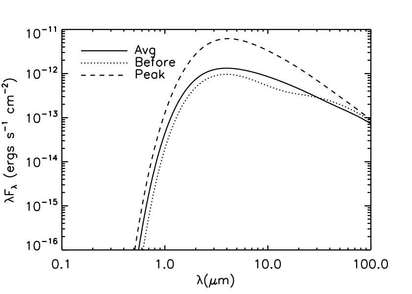
Our simulations also suggest that the disk accretion rate varies significantly at the timescale of years when the disk accretion rate is . The disk cooling timescale is also around one year for such a disk, estimated with Equation (8) in Zhu et al. (2015). Thus the change of the disk accretion rate would lead to the variability of the observables over years timescale. Thus, for these disks, the accretion tracers may vary between observations at different epochs. This is shown in Figure 11 where the dotted and dashed curves are only separated by 1.8 years but the peak intensity is differed by almost a factor of 10.
Besides disk accretion, CPDs could also launch jets/outflows (Quillen & Trilling 1998, Gressel et al. 2013), and have shock fronts due the inflow from the circumstellar disks (Tanigawa et al. 2012). They may also have observational signatures. Last but not least, the Keplerian rotation of the CPD may even be probed by molecular lines using ALMA (Perez et al. 2015).
IV.2. Satellite Formation

We can compare the disk surface density from our simulations with the disk surface density required by various satellite formation models. Our derived disk surface density is orders of magnitude smaller than the in-situ satellite formation models, or so-called the “minimum mass sub-nebula” model (Figure 12). Our simulated CPDs have surface densities between 10 and 1000 g cm-2 depending on the disk accretion rates, while the “minimum mass sub-nebula” [54, 17, 62] has a surface density of few g cm-2. The model in [62] is plotted as the dotted curve in Figure 12, which is much higher than the surface density from our 2-D simulations. On the other hand, the surface densities in our simulations are consistent with that in the “gas-starved” satellite formation model [15, 16, 85].
Since Galilean satellites are ice-rich, they need to form in conditions where the disk midplane temperature is below 150 to 200 K, depending on pressure (Prinn & Fegley 1989, Canup &Ward 2002). In order for the disk to be cooler than 200 K at R, Figure 5 suggests that the disk accretion rate needs to be smaller than or . Thus, Galilean satellites should form in a CPD with a very low accretion rate. This accretion rate is broadly consistent with that (210) suggested by Canup & Ward (2002). Using 0.001, Heller & Pudritz (2015ab) have reached the similar conclusion that Jovian moons have to form during the final stages of CPD accretion. Despite this low accretion rate, it will only take yr, well within the protoplanetary disk lifetime, for such a CPD to supply enough material for building Galilean satellites.

Although the effects of spiral shocks can be represented by the equivalent parameter as shown above, spiral shocks are substantially different from viscosity in that they can travel long distance in disks and have non-homogeneous azimuthal structure. The density and temperature are high at the shock front. Since the spiral shocks are stationary in the corotating frame, material in the CPD will move in and out of the spiral shocks during each orbit around the planet. Disk material can frequently be heated up, dissociated, and condensed again. We plot the 1-D density and temperature profiles along the azimuthal direction at 10 and 30 in Figure 13. Thus, disk material is heated episodically (twice every orbit due to the two spiral arms) and may have imprints in the material accreted onto the satellites or left in the CPD.
IV.3. Caveats
MHD effects have been completely ignored in this study. As shown in Figure 5, for disks with accretion rate larger than 10, the inner disk within 10-50 can be hot enough ( K) to sustain MRI (Keith & Wardle 2014). On the other hand, due to MRI is similar to the by the spiral shocks ( 0.001 - 0.1). Thus, the operation of MRI at the inner disk may not dramatically change the disk structure.
Previous studies (Fujii et al. 2011, 2014, Keith & Wardle 2014) find that it is difficult to sustain MRI in the majority part of the CPD beyond 30 . Non-ideal MHD effects coupled with magnetic breaking may be important there. Without efficient accretion onto the planet, mass being supplied from the circumstellar disk will pile up in CPDs, leading to gravitational instability and triggering accretion outbursts (Lubow & Martin 2012), similar to the outburst mechanism proposed for FU Orionis systems (Armitage et al. 2001, Zhu et al. 2009, Martin & Lubow 2011b). Here, we propose spiral shocks as another way to drive accretion. How this new mechanism interplays with previous proposed mechanisms needs further studies.
One of the biggest caveats in this study is that we are limited to 2-D. Previous studies (Bate et al. 2003, Machida et al. 2008, Tanigawa et al. 2012, Morbidelli et al. 2014, Szulágyi et al. 2014) have suggested that CPDs have complicated 3-D structure. Material almost falls vertically from the circumstellar disk to the CPD. Even in our 2-D simulations, is approaching 0.5 at the planet’s Hill radius (Figure 5) and our thin disk approximation breaks down there. Thus, our simulations may not accurately capture dynamics there. On the other hand, CPDs are truncated at 1/3-1/2 of the planet’s Hill radius and material around the planet’s Hill radius should not affect dynamics within CPDs. Szulágyi et al. (2016) has shown that the inner disk can undergo thermal runaway and can reach peak temperature of 10,000 K. In this case, the whole region within the Hill sphere can even become a hydrostatic envelop. Among our simulations, the case with the highest accretion rate (Gp2) may also undergo thermal runaway if we use the realistic molecular opacity and then H/R will be 0.5 at the inner disk. On the other hand, Szulágyi et al. (2016) suggests that such thermal runaway could be due to the lack of proper treatment for thermal dynamics. Nevertheless, for our other cases except Gp2, is less than 0.25 in most regions of the disk and the thin disk approximation may still be valid. Spiral shocks have complicated 3-D structure (Zhu et al. 2015, Lyra et al. 2016) and can even be unstable in 3-D (Bae et al. 2016). A proper study on how shock driven accretion is affected by the 3-D effects needs future 3-D simulations with realistic radiative transfer and thermodynamics.
V. Conclusion
Circumplanetary disks (CPD) control the growth of planets, supply material for satellites to form, and provide observational signatures of young forming planets. In this paper, we provide a new mechanism to explain how CPDs accrete.
We have carried out two dimensional hydrodynamical simulations to study CPDs using Athena++. Simple radiative cooling has been considered in the simulation. Different from most previous simulations, we choose a coordinate system centered on the planet, which significantly reduces the numerical error and enables simulations with small numerical viscosity. Our simulation domain extends from the circumstellar disk all the way to the Jupiter’s surface. A gap in the circumstellar disk is prescribed, allowing us to control the inflow rate from the circumstellar to the circumplanetary disk.
Two spiral shocks are present in CPDs, induced by the tidal force from the central star. We find that these spiral shocks can lead to significant angular momentum transport and energy dissipation in CPDs. Meanwhile, dissipation and heating by spiral shocks have a positive feedback on shock-driven accretion itself. As the disk is heated up by spiral shocks, the shocks become more open and propagate further into the inner disk, leading to more efficient angular momentum transport at the inner disk. On the other hand, shock driven accretion cannot guarantee strict steady disk accretion since the angular momentum transport depends on the global wave propagation and local shock dissipation. Mass will pile up in some regions of the disk and sometimes vortices are produced, which produce short-timescale (months to years) variability. The disk is adjusting itself through these variabilities and tries to maintain a quasi-steady state. Eventually, a quasi-steady state of accretion flow is reached in our simulations from the planet’s Hill radius all the way to the planet surface. After averaging quantities over a long timescale, angular momentum budget is carefully analyzed. The effective -coefficient characterizing angular momentum transport due to spiral shocks is 0.001-0.02 even though the disk accretion rates span 4 orders of magnitude. The value is higher in a disk with a higher accretion rate due to the shock heating feedback.
With energy budget analysis, we show that radial advection of energy becomes important and the disk generates less infrared radiation than that from the thin disk approximation by a factor of 2. Thus, if we use the infrared flux calculated from the thin disk approximation to derive the accretion rate of CPDs, we may underestimate the disk accretion rate by a factor of 2.
Finally, we calculate the flux from CPDs at ALMA and EVLA wavelength bands and predict the flux to several recent CPD candidates (e.g. HD169142b, HD100546b, LkCa 15b). These CPD candidates should be relatively bright at ALMA wavelength bands. In future, ALMA should be able to discover many accreting CPDs.
Unlike near-IR emission which comes from the inner disk region, submm flux comes from the outer disk region which is less subject to vortex production and destruction. Furthermore the dynamical time is much longer at the outer disk. Thus submm flux will be more steady over time than the optical/near-IR flux. We may see that CPDs appear and disappear between two epoch optical/near-IR observations while they are bright all the time at ALMA bands.
Although our simulations are limited to 2-D, the possibility that we may have understood how CPDs accrete and its huge implications on observations and satellite formation make it worth being studied in detail in future.
Appendix A Energy Budget
Besides studying angular momentum transport by spiral shocks, we also investigate how energy is dissipated and transported in CPDs. Understanding the energy budget during the accretion process is essential for studying the disk thermal structure and the observational signatures of disks (e.g. Spectral Energy Distributions). CPDs are quite geometrically thick with the aspect ratio reaching 0.3 (Figure 5) so that local cooling may not perfectly balance local viscous/shock heating and radial advection of energy can be important.
To calculate the energy budget, we take a similar approach as for the angular momentum equation by averaging the energy equation in the azimuthal direction
| (A1) |
The second term on the left hand side is the radial energy flux gradient which is designated as EnE+P. The first term on the right hand side, which is the gravitational potential energy released during the accretion process, is Enpot. The second term on the right hand side is the work done by the torque, EnT, while the cooling rate is Encool. Thus, the above equation is
| (A2) |
which basically states that the energy change is due to the flux into the domain, the work done by forces (the gravitational force from the central object and other forces), and radiative cooling. After being normalized with , all these terms for case Gp2 are plotted in the left panel of Figure 14. Figure 14 suggests that the work done by the torque is negligible at the inner disk and the cooling rate equals the difference between the released potential energy and the energy flux gradient.

After removing second order terms, EnE+P can be expanded as
| (A3) |
With , the above equation becomes
| (A4) |
The three terms on the right hand side are the gradient of kinetic energy, Reynolds stress, and the pressure. Thus, we designate the three terms as Enkic, EnRey, and Enpre, and we have
| (A5) |
Note that actually consists of two parts: one is the advection of the internal energy and the other is related to the work done by the pressure.
If we assume that the disk accretion rate is a constant, we can replace the Reynolds stress with the disk accretion rate by using Eq. 17
| (A6) | ||||
where we have further neglected the external force term, and designate the first and second term as En and EnConst. Thus, finally we have
| (A7) |
If we assume and , and normalize Equation A1 with (designate the corresponding quantities with a hat symbol), we have
and thus
| (A8) |
If we assume zero stress at and neglect the pressure term, as in the thin disk approximation, we have derived in §3.2. Thus
| (A9) |
Among the total cooling rate,1 comes from the release of the gravitational energy, and 1/2-3/2 comes from the radial energy transport. Except the very inner disk, the radial energy transport normally heats up the disk. -3/2 in the radial transported energy is from the zero torque boundary condition (Shakura & Sunyaev 1973).
To compare all the energy terms derived directly from our simulations with the corresponding terms in the thin disk approximation, we summarize all the normalized energy terms in the thin disk theory
| (A10) | ||||
| (A11) | ||||
| (A12) | ||||
| (A13) | ||||
| (A14) | ||||
| (A15) | ||||
| (A16) | ||||
| (A17) |
Thus,
| (A18) | ||||
| (A19) |
and, eventually,
| (A20) |
The normalized quantities in the thin disk approximation are plotted in the right panel of Figure 14.

By comparing the left and right panels in Figure 14 where all quantities have been normalized by 8G/, we can see that the cooling rate in the simulation is smaller than the cooling rate derived from the thin disk approximation, especially at the outer disk. The ratio between the cooling rate from simulations and that from the thin disk approximation is shown in Figure 15. Clearly, the cooling rate is only half of that predicted in the thin disk theory at . Based on the relation in Equation A10, this lower cooling rate in real simulations is caused by the higher value of . A higher value means that the radial energy transport depletes more energy from the disk.
To understand why is higher in simulations, we plot different components of in Figure 16. By comparing the real simulations (the left panel) with the thin disk approximation (the right panel), we can see that the pressure term (Enpre) which represents the radial advection of both the internal energy and the pressure is non-negligible in the simulation. It is negative at the inner disk within 4 and positive at the outer disk. Thus, the inner disk loses energy and the outer disk gains energy due to the non-zero Enpre term. This non-negligible radial transport of energy makes the CPD more like a ”slim disk” (Abramowicz et al. 1988) than a thin disk.
We also notice that almost balances the Reynolds stress term (), so that the total energy flux gradient term () is almost equal to the kinetic energy term (). Thus, empirically, we can approximate as 1/2 instead of in the thin disk theory. The new cooling rate is thus 1/2. If we relate the cooling rate with the effective temperature (), we can derive the effective temperature in the CPD as
| (A21) |
which is significantly different from the temperature in the thin disk theory (Equation A20). Thus, compared with the thin disk, the simulated disk is hotter at the inner disk and cooler at the outer disk. We want to emphasize that Equation A21 which assumes 1/2 is an empirical approximation, it slightly overestimates the inner disk temperature compared with real simulations as shown in Figure 14 where is smaller than 1/2 at the inner disk.
Overall, our simulations show different temperature profiles from the thin disk theory. This difference is not caused by the boundary condition since the zero stress boundary condition also stands in our simulations as discussed at the end of §3.2. Instead, the difference is caused by the radial advection of energy since H/R is large and the thin disk approximation is not valid anymore in the CPD.

References
- [1] Abramowicz, M. A., Czerny, B., Lasota, J. P., & Szuszkiewicz, E. 1988, ApJ, 332, 646
- [2] Alcalá, J. M., Natta, A., Manara, C. F., et al. 2014, A&A, 561, A2
- [3] Andrews, S. M., Wilner, D. J., Hughes, A. M., et al. 2012, ApJ, 744, 162
- [4] Armitage, P. J., Livio, M., & Pringle, J. E. 2001, MNRAS, 324, 705
- [5] Ayliffe, B. A., & Bate, M. R. 2009, MNRAS, 397, 657
- [6] Bae, J., Nelson, R. P., Hartmann, L., & Richard, S. 2016, ApJ, 829, 13
- [7] Balbus, S. A., & Hawley, J. F. 1998, Reviews of Modern Physics, 70, 1
- [8] Bate, M. R., Lubow, S. H., Ogilvie, G. I., & Miller, K. A. 2003, MNRAS, 341, 213
- [9] Bai, X.-N. 2014, ApJ, 791, 137
- [10] Belyaev, M. A., Rafikov, R. R., & Stone, J. M. 2013, ApJ, 770, 67
- [11] Biller, B. A., Males, J., Rodigas, T., et al. 2014, ApJ, 792, L22
- [12] Bowler, B. P., Andrews, S. M., Kraus, A. L., et al. 2015, ApJ, 805, L17
- [13] Bouvier, J., Alencar, S. H. P., Harries, T. J., Johns-Krull, C. M., & Romanova, M. M. 2007, Protostars and Planets V, 479
- [14] Calvet, N., & Gullbring, E. 1998, ApJ, 509, 802
- [15] Canup, R. M., & Ward, W. R. 2002, AJ, 124, 3404
- [16] Canup, R. M., & Ward, W. R. 2006, Nature, 441, 834
- [17] Coradini, A., & Magni, G. 1984, ICARUS, 59, 376
- [18] Currie, T., Cloutier, R., Brittain, S., et al. 2015, ApJ, 814, L27
- [19] D’Alessio, P., Calvet, N., & Hartmann, L. 2001, ApJ, 553, 321
- [20] D’Angelo, G., Henning, T., & Kley, W. 2003, ApJ, 599, 548
- [21] D’Angelo, G., & Podolak, M. 2015, ApJ, 806, 203
- [22] de Val-Borro, M., Edgar, R. G., Artymowicz, P., et al. 2006, MNRAS, 370, 529
- [23] Fendt, C. 2003, A&A, 411, 623
- [24] Fujii, Y. I., Okuzumi, S., & Inutsuka, S.-i. 2011, ApJ, 743, 53
- [25] Fujii, Y. I., Okuzumi, S., Tanigawa, T., & Inutsuka, S.-i. 2014, ApJ, 785, 101
- [26] Fung, J., Shi, J.-M., & Chiang, E. 2014, ApJ, 782, 88
- [27] Gammie, C. F. 1996, ApJ, 457, 355
- [28] Gardiner, T. A., & Stone, J. M. 2005, Journal of Computational Physics, 205, 509
- [29] Gardiner, T. A., & Stone, J. M. 2008, Journal of Computational Physics, 227, 4123
- [30] Goodman, J., & Rafikov, R. R. 2001, ApJ, 552, 793
- [31] Gressel, O., Nelson, R. P., Turner, N. J., & Ziegler, U. 2013, ApJ, 779, 59
- [32] Gullbring, E., Calvet, N., Muzerolle, J., & Hartmann, L. 2000, ApJ, 544, 927
- [33] Hartmann, L., Hewett, R., & Calvet, N. 1994, ApJ, 426, 669
- [34] Hayashi, C. 1981, Progress of Theoretical Physics Supplement, 70, 35
- [35] Heller, R., & Pudritz, R. 2015a, A&A, 578, A19
- [36] Heller, R., & Pudritz, R. 2015b, ApJ, 806, 181
- [37] Herczeg, G. J., & Hillenbrand, L. A. 2008, ApJ, 681, 594-625
- [38] Hernández, J., Hartmann, L., Megeath, T., et al. 2007, ApJ, 662, 1067
- [39] Hubeny, I. 1990, ApJ, 351, 632
- [40] Ingleby, L., Calvet, N., Herczeg, G., et al. 2013, ApJ, 767, 112
- [41] Isella, A., Chandler, C. J., Carpenter, J. M., Pérez, L. M., & Ricci, L. 2014, ApJ, 788, 129
- [42] Ju, W., Stone, J. M., & Zhu, Z. 2016, arXiv:1604.00715
- [43] Keith, S. L., & Wardle, M. 2014, MNRAS, 440, 89
- [44] Kley, W., & Nelson, R. P. 2012, ARA&A, 50, 211
- [45] Kraus, A. L., & Ireland, M. J. 2012, ApJ, 745, 5
- [46] Kunz, M. W., & Lesur, G. 2013, MNRAS, 434, 2295
- [47] Larson, R. B. 1990, MNRAS, 243, 588
- [48] Lesur, G., Kunz, M. W., & Fromang, S. 2014, A&A, 566, A56
- [49] Lin, D. N. C., & Papaloizou, J. 1986, ApJ, 309, 846
- [50] Lovelace, R. V. E., Li, H., Colgate, S. A., & Nelson, A. F. 1999, ApJ, 513, 805
- [51] Lovelace, R. V. E., Covey, K. R., & Lloyd, J. P. 2011, AJ, 141, 51
- [52] Lubow, S. H., Seibert, M., & Artymowicz, P. 1999, ApJ, 526, 1001
- [53] Lubow, S. H., & Martin, R. G. 2012, ApJ, 749, L37
- [54] Lunine, J. I., & Stevenson, D. J. 1982, ICARUS, 52, 14
- [55] Lyra, W., Richert, A. J. W., Boley, A., et al. 2016, ApJ, 817, 102
- [56] Machida, M. N., Kokubo, E., Inutsuka, S.-i., & Matsumoto, T. 2008, ApJ, 685, 1220
- [57] Machida, M. N. 2009, MNRAS, 392, 514
- [58] Marley, M. S., Fortney, J. J., Hubickyj, O., Bodenheimer, P., & Lissauer, J. J. 2007, ApJ, 655, 541
- [59] Martin, R. G., & Lubow, S. H. 2011a, MNRAS, 413, 1447
- [60] Martin, R. G., & Lubow, S. H. 2011b, ApJ, 740, L6
- [61] Morbidelli, A., Szulágyi, J., Crida, A., et al. 2014, ICARUS, 232, 266
- [62] Mosqueira, I., & Estrada, P. R. 2003, ICARUS, 163, 198
- [63] Muzerolle, J., Calvet, N., & Hartmann, L. 1998, ApJ, 492, 743
- [64] Muzerolle, J., Calvet, N., & Hartmann, L. 2001, ApJ, 550, 944
- [65] Owen, J. E. 2014, ApJ, 789, 59
- [66] Owen, J. E., & Menou, K. 2016, ApJ, 819, L14
- [67] Paardekooper, S.-J., Lesur, G., & Papaloizou, J. C. B. 2010, ApJ, 725, 146
- [68] Papaloizou, J. C. B., & Nelson, R. P. 2005, A&A, 433, 247
- [69] Perez, S., Dunhill, A., Casassus, S., et al. 2015, ApJ, 811, L5
- [70] Philippov, A. A., Rafikov, R. R., & Stone, J. M. 2016, ApJ, 817, 62
- [71] Prinn, R. G. P., & Fegley, B., Jr. 1989, Origin and Evolution of Planetary and Satellite Atmospheres, 78
- [72] Quanz, S. P., Amara, A., Meyer, M. R., et al. 2013, ApJ, 766, L1
- [73] Quanz, S. P., Amara, A., Meyer, M. R., et al. 2015, ApJ, 807, 64
- [74] Quillen, A. C., & Trilling, D. E. 1998, ApJ, 508, 707
- [75] Reggiani, M., Quanz, S. P., Meyer, M. R., et al. 2014, ApJ, 792, L23
- [76] Rigliaco, E., Natta, A., Testi, L., et al. 2012, A&A, 548, A56
- [77] Rivier, G., Crida, A., Morbidelli, A., & Brouet, Y. 2012, A&A, 548, A116
- [78] Sallum, S., Follette, K. B., Eisner, J. A., et al. 2015, Nature, 527, 342
- [79] Shakura, N. I., & Sunyaev, R. A. 1973, A&A, 24, 337
- [80] Spiegel, D. S., & Burrows, A. 2012, ApJ, 745, 174 (SB)
- [81] Spruit, H. C. 1987, A&A, 184, 173
- [82] Stone, J. M., Gardiner, T. A., Teuben, P., Hawley, J. F., & Simon, J. B. 2008, ApJS, 178, 137
- [83] Szulágyi, J., Morbidelli, A., Crida, A., & Masset, F. 2014, ApJ, 782, 65
- [84] Szulágyi, J., Masset, F., Lega, E., et al. 2016, arXiv:1605.04586
- [85] Ward, W. R., & Canup, R. M. 2010, AJ, 140, 1168
- [86] Tanigawa, T., Ohtsuki, K., & Machida, M. N. 2012, ApJ, 747, 47
- [87] Turner, N. J., Lee, M. H., & Sano, T. 2014, ApJ, 783, 14
- [88] Zhou, Y., Herczeg, G. J., Kraus, A. L., Metchev, S., & Cruz, K. L. 2014, ApJ, 783, L17
- [89] Zhu, Z., Hartmann, L., Calvet, N., Hernandez, J., Muzerolle, J., & Tannirkulam, A.-K. 2007, ApJ, 669, 483
- [90] Zhu, Z., Hartmann, L., & Gammie, C. 2009, ApJ, 694, 1045
- [91] Zhu, Z., Stone, J. M., & Rafikov, R. R. 2013, ApJ, 768, 143
- [92] Zhu, Z., Dong, R., Stone, J. M., & Rafikov, R. R. 2015, ApJ, 813, 88
- [93] Zhu, Z. 2015, ApJ, 799, 16