Estimation of Graphical Models through Structured Norm Minimization

Let $X$ be an $m\times p$ data matrix, $\Theta$ be a $p\times p$ symmetric matrix containing the parameters of interest of the statistical loss function $\mathcal{G}(X,\Theta)$. The most popular assumption used in the literature is that $\Theta$ is sparse and can be successfully recovered from high-dimensional data by solving the following optimization problem

where $\mathcal{S}$ is some set depending on the loss function; $\lambda$ is s a non-negative regularization constant; and $\|.\|_{1}$ denotes the $\ell_{1}$ norm or the sum of the absolute values of the matrix elements.

To explicitly model different structures in the parameter $\Theta$, we introduce the following symmetric structured overlap norm (SSON):

We note that the overlap norm defined by Mohan et al. (2012); Tan et al. (2014) encourages the recovery of matrices that can be expressed as a union of few rows and the corresponding columns (i.e. hub nodes). However, SSON represents a new symmetric and significantly more general variant of the overlap norm that promotes matrices that can be expressed as the sum of symmetric structured matrices. Moreover, unlike the previous group sparsity and the latent group lasso discussed in Yuan and Lin (2007); Jacob et al. (2009); Obozinski et al. (2011) that require users to specify structures of interest a priori, the SSON achieves a similar objective in an agnostic manner, relying only on how well such structures fit the observed data.

In many applications, such as regression models, we are interested in modeling different structures in a parameter vector $\theta$. In these cases, we have the following definition as a special case of SSON:

Note that SSON is rather different from the sparse group lasso, which also uses a combination of $\ell_{1}$ and $\ell_{G}$ penalization, where $\|.\|_{G}$ is the group lasso norm. The sparse group lasso penalty is $\bar{\omega}(\theta)=\lambda_{1}\|\theta\|_{1}+\lambda_{2}\|\theta\|_{G}$, and thus the includes lasso and group lasso as extreme cases corresponding to $\lambda_{2}=0$ and $\lambda_{1}=0$, respectively. However, $\bar{\omega}(\theta)$ does not split $\theta$ into a sparse and a group sparse part and will produce a sparse solution as long as $\lambda_{1}>0$. Hence, the sparse group lasso method can be thought of as a sparsity-based method with additional shrinkage by $\|\theta\|_{G}$. The group sparsity processes data very differently from SSON and consequently has very different prediction risk behavior. The same argument illustrates the advantages of the proposed SSON penalty over the well-known elastic net penalty. The elastic net is a combination of lasso and ridge penalties (Zou and Hastie, 2005). However, the elastic net does not split $\theta$ into a sparse and a dense component. Our results show that SSON tends to perform no worse than, and often performs significantly better than ridge, lasso, group lasso or elastic net with penalty levels chosen by cross-validation.

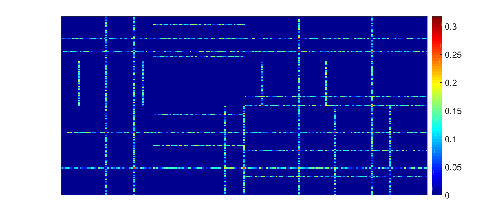
Next, we discuss the use of the SSON as a regularizer for maximum likelihood estimation of the following popular statistical models: (i) members of the Markov Random Field family including the Gaussian graphical model, the Gaussian graphical model with latent variables and the binary Ising model, (ii) the Gaussian covariance graph model and (iii) the classical regression and the vector auto-regression models. For the sake of completeness, we provide a complete, but succinct description of the corresponding models and the proposed regularization.

Let $X$ be a data matrix consisting of $p$-dimensional samples from a zero mean Gaussian distribution,

In order to obtain a sparse and interpretable estimate of the precision matrix $\Sigma^{-1}$ that captures conditional dependence relationships, many authors have considered the well-known graphical lasso problem (Friedman et al., 2008; Rothman et al., 2008) in the form of (2) with loss function

where $\hat{\Sigma}$ is the empirical covariance matrix of $X$; $\Theta_{1}$ is the estimate of the precision matrix $\Sigma^{-1}$; and $\mathcal{S}$ is the set of $p\times p$ symmetric positive definite matrices.

As is well known, the norm penalty in (2) encourages zeros (sparsity) in the solution. However, as previously argued, many biological and social network applications exhibit more complex structures than mere sparsity. Using the proposed SSON, we define the following objective function for the problem at hand:

where $\Theta_{1}$ is the model parameter matrix and $\Omega(\Theta_{1},Z_{1},\dots,Z_{n},E)$ the corresponding SSON defined in (3).

Formulation (6) allows us to obtain more accurate and compact network estimates than conventional methods whenever the network exhibits different structures. Moreover, our formulation does not require a priori knowledge of the underlying network structure (i.e. which nodes in the network form densely connected subgraphs (see, Figure 4)).

In Figure 4, the performance of our proposed approach is illustrated on two simulated data sets exhibiting different structures (sub-figures (4(c)) and (4(f))); it can be seen that the proposed SSON based graphical lasso (sub-figures (4(b)) and (4(e))) can recover the network structure much better than the popular graphical lasso based estimator (Friedman et al., 2008) (subfigures (4(a)) and (4(d))).

Another popular graphical model, suitable for binary or categorical data, is the Ising one (Ising, 1925). It is assumed that observations $x_{1},\dots,x_{m}$ are independent and identically distributed from

where $\mathbb{W}(\Theta_{2})$ is the partition function, which ensures that the density sums to one. Here, $\Theta_{2}$ is a $p\times p$ symmetric matrix that specifies the network structure: $\theta_{jj^{\prime}}=0$ implies that the $j$th and $j^{\prime}$th variables are conditionally independent given the remaining ones.

Several papers proposing estimation procedures for this model have been published. Lee et al. (2007) considered maximizing an $\ell_{1}$-penalized log-likelihood for this model. Due to the difficulty in computing the log-likelihood with the expensive partition function, several authors have considered alternative approaches. For instance, Ravikumar et al. (2011) proposed a neighborhood selection approach. The latter proposal involves solving $p$ logistic regressions separately (one for each node in the network), which leads to an estimated parameter matrix that is in general not symmetric. In contrast, several authors considered maximizing an $\ell_{1}$-penalized pseudo-likelihood with a symmetric constraint on $\Theta_{2}$ (Guo et al., 2011a; Guo et al., 2011b). Under the model (7), the $\log$-pseudo-likelihood for $m$ observations takes the form

We propose instead to impose the SSON on $\Theta_{2}$ in (8) in order to estimate a binary network with different structures. This leads to the following optimization problem

where $\Theta_{2}$ is the model parameter matrix and $\Omega(\Theta_{2},Z_{1},\dots,Z_{n},E)$ the corresponding SSON defined in (3).

An interesting connection can be drawn between our technique and the Ising block model discussed in Berthet et al. (2016), which is a perturbation of the mean field approximation of the Ising model known as the Curie-Weiss model: the sites are partitioned into two blocks of equal size and the interaction between those within the same block is stronger than across blocks, to account for more order within each block. However, one can easily seen that the Ising block model is a special case of (9).

Next, we consider estimation of a covariance matrix under the assumption that

This is of interest because the sparsity pattern of $\Sigma$ specifies the structure of the marginal independence graph (Drton and Richardson, 2002; Drton and Richardson, 2008).

Let $\Theta_{3}$ be a $p\times p$ symmetric matrix containing the parameters of interest. Setting the loss function $\mathcal{G}_{3}(X,\Theta_{3}):=\dfrac{1}{2}\|\Theta_{3}-\hat{\Sigma}\|^{2}_{F}$, Xue et al. (2012) proposed to estimate the positive definite covariance matrix, $\Sigma$ by solving

where $\hat{\Sigma}$ is the empirical covariance matrix, $\mathcal{S}=\{\Theta_{3}:\Theta_{3}\succeq\varepsilon I\text{ and }\Theta_{3}=\Theta^{T}_{3}\}$, and $\varepsilon$ is a small positive constant. We extend (10) to accommodate structures of the covariance graph by imposing the SSON on $\Theta_{3}$. This results in the following optimization problem

where $\Theta_{3}$ is the model parameter matrix and $\Omega(\Theta_{3},Z_{1},\dots,Z_{n},E)$ the corresponding SSON defined in (3).

In many applications throughout science and engineering, it is often the case that some relevant variables are not observed. For the Gaussian Graphical model, Chandrasekaran et al. (2010) proposed a convex optimization problem to estimate it in the presence of latent variables. Let $\Theta_{4}$ be a $p\times p$ symmetric matrix containing the parameters of interest. Setting $\mathcal{G}_{4}(X,\Theta_{4}):=\langle\Theta_{4},\Sigma_{O}\rangle-\log\det\Theta_{4}$, their objective function is given by

where $\Sigma_{O}$ is the sample covariance matrix of the observed variables; $\alpha$ and $\beta$ are positive constants; and the indicator function $\mathbbm{1}_{Z_{n+1}\succeq 0}$ is defined as

This convex optimization problem aims to estimate an inverse covariance matrix that can be decomposed into a sparse matrix $Z_{1}$ minus a low-rank matrix $Z_{n+1}$ based on high-dimensional data.

Next, we extend the SSON to solve the latent variable graphical model selection. Problem (12) can be rewritten in the following equivalent form by introducing new variables $\{Z_{i}\}_{i=1}^{n}$:

where $\Theta_{4}$ is the model parameter matrix and $\Omega(\Theta_{4},Z_{1},\dots,Z_{n},E)$ the corresponding SSON defined in (3).

The proposed SSON is also applicable to structured regression problems. Although this is not the main focus on this paper, nevertheless, we include a brief discussion, especially for lag selection in vector autoregressive models that are of prime interest in the analysis of high-dimensional time series data. The canonical formulation of the regularized regression problem is given by:

where $\{(y_{i},x_{i})\}_{i=1}^{m}$, $y_{i}\in\mathbb{R}$, $x_{i}\in\mathbb{R}^{p}$, with $y=[y_{1},\dots,y_{m}]^{\top}$ being the response variable and $X=[x_{1}^{\top},\dots x_{m}^{\top}]$ a set of $p$-predictors that are assumed to be independently and identically distributed (i.i.d.); $\lambda>0$ is a regularization parameter and $\Psi(\theta)$ is a suitable norm. Specific choices of $\Psi(.)$ lead to popular regularizers including the lasso -$\Psi(\theta)=\|\theta\|_{1}$- and the group lasso.

We propose instead to impose the SSON on $\theta$ in (14) in order to solve structured regression problems. Problem (14) can be rewritten in the following form by introducing new variables $\{z_{i}\}_{i=1}^{n}$ and $e$:

where $\mathcal{G}(X,\theta)=\|y-X\theta\|_{2}$; $\theta$ is the model parameter vector and $\omega(\theta,z_{1},\dots,z_{n},e)$ the corresponding structured norm defined in (4).

Problem (15) can equivalently be thought of as a generalization of subspace clustering (Elhamifar and Vidal, 2009). Indeed, in order to segment the data into their respective subspaces, we need to compute an affinity vector $\theta$ that encodes the pairwise affinities between data vectors.

An interesting application of the SSON for multivariate regression problems is on structured estimation of vector autoregression (VAR) models (Lütkepohl, 2005), a popular model for economic and financial time series data (Tsay, 2005), dynamical systems (Ljung, 1998) and more recently brain function connectivity (Valdés-Sosa et al., 2005). The model captures both temporal and cross-dependencies between stationary time series. Formally, let $\{x_{1},\dots,x_{m}\}$ be a $p$-dimensional time series set of observations that evolve over time according to a lag-$d$ model:

where $\{\Theta\}_{k=1}^{d}\in\mathbb{R}^{p\times p}$ are transition matrices for different lags, and $\{\epsilon_{1},\ldots,\epsilon_{m-1}\}$ independent multivariate Gaussian white noise processes. The VAR process is assumed to be stable and stationary (bounded spectral density), while the noise covariance matrix $\Sigma$ is assumed to be positive definite with bounded largest eigenvalue (Basu and Michailidis, 2015).

Given $m$ observations $\{x_{1},x_{2},\dots,x_{m}\}$ from a stationary VAR process, the lag-$m$ VAR can be written is given by

It can be seen that to estimate $\Theta$ one can solve the following least squares problem

However, as the number of component time series increases, the number of parameters to be estimated grows as $dp^{2}$ ; hence, structural assumptions are imposed to estimate them from limited sample size. A popular choice is the lasso (Basu and Michailidis, 2015), that leads to sparse estimates. However, it does not incorporate the notion of lag selection, which could lead to certain spurious coefficients coming from further lags in the past. To address this problem, Basu et al. (2015) proposed a thresholded lasso estimate. However, our SSON can be used for lag selection, that guarantees that more recent lags are favored over further in the past ones.

Let $\Theta_{5}$ be a $mp\times mp$ symmetric matrix containing the parameters of interest for all $m$ lages of the problem. Setting the loss function $\mathcal{G}_{5}(X,\Theta_{5}):=\|Y-X\Theta_{5}\|$, we propose to estimate the transition matrix, $\Theta$ by solving the following optimization problem:

where $\Theta_{5}$ is the estimate of the covariance matrix and $\Omega(\Theta_{5},Z_{1},\dots,Z_{n},E)$ the corresponding SSON defined in (3).

The next result establishes the global convergence of the standard multi-block ADMM for solving SSON based statistical learning problems, by using the Kurdyka- Lojasiewicz (KL) property of the objective function in (19).

Proof. A detailed exposition is given in Appendix B.

Next, we evaluate the performance of SSONA on ten synthetic graphical model problems, comprising of $p=100$, 500 and 1000 variables. The underlying network structure corresponds to an Erdős-Rényi model graph, a nearest neighbor graph and a scale-free random graph, respectively. The CONTEST ¹¹ 1 CONTEST is available at http://www.mathstat.strath.ac.uk/outreach/contest/ package is used to generate the synthetic graphs, and the UGM ²² 2 UGM is available at http://www.di.ens.fr/ mschmidt/Software/UGM.html package to implement Gibbs sampling for estimating the Ising Model. Based on the generated graph topologies, we consider the following settings for generating synthetic data sets:

• I.

  Gaussian graphical models:
  For a given number of variables $p$, we first create a symmetric matrix $E\in\mathbb{R}^{p\times p}$ by using CONTEST in a MATLAB environment. Given matrix $E$, we set $\Sigma^{-1}$ equal to $E+(0.1-\bar{\Lambda}_{\min}(E))~I$, where $\bar{\Lambda}_{\min}(E)$ is the smallest eigenvalue of $E$ and $I$ denotes the identity matrix. We then draw $N=5p$ i.i.d. vectors $x_{1},\dots,x_{m}$ from the gasserian distribution $\mathcal{N}(0,\Sigma)$ by using the mvnrnd function in MATLAB, and then compute a sample covariance matrix of the variables.

• II.

  Gaussian graphical models with latent variables:
  For a given number of variables $p$, we first create a matrix $\Sigma^{-1}\in\mathbb{R}^{(p+r)\times(p+r)}$ by using CONTEST as described in I. We then choose the sub-matrix $\Theta_{O}=\Sigma^{-1}(1:p,1:p)$ as the ground truth matrix of the matrix $\Theta_{4}$ and chose

  	$\displaystyle\Theta_{U}$	$\displaystyle=$	$\displaystyle\Sigma^{-1}(1:p,~p+1:p+r)\big(\Sigma^{-1}(p+1:p+r,~p+r:p+r)\big)^{-1}$
  			$\displaystyle\Sigma^{-1}(p+1:p+r,~1:p)$

  as the ground truth matrix of the low rank matrix $U$. We then draw $N=5p$ i.i.d. vectors $x_{1},\dots,x_{m}$ from the Gaussian distribution $\mathcal{N}(0,(\Theta_{O}-\Theta_{U})^{-1})$, and compute the sample covariance matrix of the variables $\Sigma_{O}$.

• III.

  The Binary Network:
  To generate the parameter matrix $\Sigma$, we create an adjacency matrix as in Setup I by using CONTEST. Then, each of $N=5p$ observations is generated through Gibbs sampling. We take the first 100000 iterations as our burn-in period, and then collect observations, so that they are nearly independent.

References

- Ataee Tarzanagh et al. (2014) D Ataee Tarzanagh, M Reza Peyghami, and H Mesgarani. A new nonmonotone trust region method for unconstrained optimization equipped by an efficient adaptive radius. Optimization Methods and Software, 29(4):819–836, 2014.
- Barabási and Albert (1999) Albert-László Barabási and Réka Albert. Emergence of scaling in random networks. science, 286(5439):509–512, 1999.
- Barzilai and Borwein (1988) Jonathan Barzilai and Jonathan M Borwein. Two-point step size gradient methods. IMA journal of numerical analysis, 8(1):141–148, 1988.
- Basu and Michailidis (2015) Sumanta Basu and George Michailidis. Regularized estimation in sparse high-dimensional time series models. The Annals of Statistics, 43(4):1535–1567, 2015.
- Basu et al. (2015) Sumanta Basu, Ali Shojaie, and George Michailidis. Network granger causality with inherent grouping structure. The Journal of Machine Learning Research, 16(1):417–453, 2015.
- Berthet et al. (2016) Quentin Berthet, Philippe Rigollet, and Piyush Srivastava. Exact recovery in the Ising block model. arXiv:1612.03880, 2016.
- Blei et al. (2003) David M Blei, Andrew Y Ng, and Michael I Jordan. Latent dirichlet allocation. Journal of machine Learning research, 3(Jan):993–1022, 2003.
- Bolte et al. (2014) Jérôme Bolte, Shoham Sabach, and Marc Teboulle. Proximal alternating linearized minimization for nonconvex and nonsmooth problems. Mathematical Programming, 146(1-2):459–494, 2014.
- Boyd et al. (2011) Stephen Boyd, Neal Parikh, Eric Chu, Borja Peleato, and Jonathan Eckstein. Distributed optimization and statistical learning via the alternating direction method of multipliers. Foundations and Trends® in Machine Learning, 3(1):1–122, 2011.
- Cai and Liu (2011) Tony Cai and Weidong Liu. Adaptive thresholding for sparse covariance matrix estimation. Journal of the American Statistical Association, 106(494):672–684, 2011.
- Chandrasekaran et al. (2010) Venkat Chandrasekaran, Pablo A Parrilo, and Alan S Willsky. Latent variable graphical model selection via convex optimization. In Communication, Control, and Computing (Allerton), 2010 48th Annual Allerton Conference on, pages 1610–1613. IEEE, 2010.
- Chen et al. (2016) Caihua Chen, Bingsheng He, Yinyu Ye, and Xiaoming Yuan. The direct extension of admm for multi-block convex minimization problems is not necessarily convergent. Mathematical Programming, 155(1-2):57–79, 2016.
- Chernozhukov et al. (2017) Victor Chernozhukov, Christian Hansen, and Yuan Liao. A lava attack on the recovery of sums of dense and sparse signals. The Annals of Statistics, 45(1):39–76, 2017.
- Danaher et al. (2014) Patrick Danaher, Pei Wang, and Daniela M Witten. The joint graphical lasso for inverse covariance estimation across multiple classes. Journal of the Royal Statistical Society: Series B (Statistical Methodology), 76(2):373–397, 2014.
- Davis and Yin (2015) Damek Davis and Wotao Yin. A three-operator splitting scheme and its optimization applications. Set-Valued and Variational Analysis, pages 1–30, 2015.
- Dolan and Moré (2002) Elizabeth D Dolan and Jorge J Moré. Benchmarking optimization software with performance profiles. Mathematical programming, 91(2):201–213, 2002.
- Drton and Richardson (2002) Mathias Drton and Thomas S Richardson. A new algorithm for maximum likelihood estimation in gaussian graphical models for marginal independence. In Proceedings of the Nineteenth conference on Uncertainty in Artificial Intelligence, pages 184–191. Morgan Kaufmann Publishers Inc., 2002.
- Drton and Richardson (2008) Mathias Drton and Thomas S Richardson. Graphical methods for efficient likelihood inference in gaussian covariance models. Journal of Machine Learning Research, 9(May):893–914, 2008.
- Elhamifar and Vidal (2009) Ehsan Elhamifar and René Vidal. Sparse subspace clustering. In Computer Vision and Pattern Recognition, 2009. CVPR 2009. IEEE Conference on, pages 2790–2797. IEEE, 2009.
- Fletcher (2005) Roger Fletcher. On the barzilai-borwein method. Optimization and control with applications, pages 235–256, 2005.
- Fortunato (2010) Santo Fortunato. Community detection in graphs. Physics reports, 486(3):75–174, 2010.
- Friedman et al. (2008) Jerome Friedman, Trevor Hastie, and Robert Tibshirani. Sparse inverse covariance estimation with the graphical lasso. Biostatistics, 9(3):432–441, 2008.
- Guimera and Amaral (2005) Roger Guimera and Luis A Nunes Amaral. Functional cartography of complex metabolic networks. Nature, 433(7028):895–900, 2005.
- Guo et al. (2011a) Jian Guo, Elizaveta Levina, George Michailidis, and Ji Zhu. Joint estimation of multiple graphical models. Biometrika, 98(1):1–15, 2011a.
- Guo et al. (2011b) Jian Guo, Elizaveta Levina, George Michailidis, and Ji Zhu. Asymptotic properties of the joint neighborhood selection method for estimating categorical markov networks. arXiv preprint math.PR/0000000, 2011b.
- Guo et al. (2015) Jian Guo, Jie Cheng, Elizaveta Levina, George Michailidis, and Ji Zhu. Estimating heterogeneous graphical models for discrete data with an application to roll call voting. The Annals of Applied Statistics, 9(2):821, 2015.
- Hajinezhad and Hong (2015) Davood Hajinezhad and Mingyi Hong. Nonconvex alternating direction method of multipliers for distributed sparse principal component analysis. In Signal and Information Processing (GlobalSIP), 2015 IEEE Global Conference on, pages 255–259. IEEE, 2015.
- Hajinezhad et al. (2016) Davood Hajinezhad, Mingyi Hong, Tuo Zhao, and Zhaoran Wang. Nestt: A nonconvex primal-dual splitting method for distributed and stochastic optimization. In Advances in Neural Information Processing Systems, pages 3215–3223, 2016.
- Hoerl and Kennard (1970) Arthur E Hoerl and Robert W Kennard. Ridge regression: Biased estimation for nonorthogonal problems. Technometrics, 12(1):55–67, 1970.
- Höfling and Tibshirani (2009) Holger Höfling and Robert Tibshirani. Estimation of sparse binary pairwise markov networks using pseudo-likelihoods. Journal of Machine Learning Research, 10(Apr):883–906, 2009.
- Hong and Luo (2017) Mingyi Hong and Zhi-Quan Luo. On the linear convergence of the alternating direction method of multipliers. Mathematical Programming, 162(1-2):165–199, 2017.
- Ising (1925) Ernst Ising. Beitrag zur theorie des ferromagnetismus. Zeitschrift für Physik A Hadrons and Nuclei, 31(1):253–258, 1925.
- Jacob et al. (2009) Laurent Jacob, Guillaume Obozinski, and Jean-Philippe Vert. Group lasso with overlap and graph lasso. In Proceedings of the 26th annual international conference on machine learning, pages 433–440. ACM, 2009.
- Karoui (2008) Noureddine El Karoui. Operator norm consistent estimation of large-dimensional sparse covariance matrices. The Annals of Statistics, pages 2717–2756, 2008.
- Lee et al. (2007) Su-In Lee, Varun Ganapathi, and Daphne Koller. Efficient structure learning of Markov networks using -regularization. In Advances in neural Information processing systems, pages 817–824, 2007.
- Lewis et al. (2010) Anna CF Lewis, Charlotte M Deane, Mason A Porter, and Nick S Jones. The function of communities in protein interaction networks at multiple scales. BMC systems biology, 4(1):100, 2010.
- Li et al. (2005) Lun Li, David Alderson, John C Doyle, and Walter Willinger. Towards a theory of scale-free graphs: Definition, properties, and implications. Internet Mathematics, 2(4):431–523, 2005.
- Liljeros et al. (2001) Fredrik Liljeros, Christofer R Edling, Luis A Nunes Amaral, H Eugene Stanley, and Yvonne Åberg. The web of human sexual contacts. Nature, 411(6840):907–908, 2001.
- Lin et al. (2015) Tianyi Lin, Shiqian Ma, and Shuzhong Zhang. On the global linear convergence of the ADMM with multiblock variables. SIAM Journal on Optimization, 25(3):1478–1497, 2015.
- Lin et al. (2016) Tianyi Lin, Shiqian Ma, and Shuzhong Zhang. Iteration complexity analysis of multi-block ADMM for a family of convex minimization without strong convexity. Journal of Scientific Computing, 69(1):52–81, 2016.
- Lin et al. (2011) Zhouchen Lin, Risheng Liu, and Zhixun Su. Linearized alternating direction method with adaptive penalty for low-rank representation. In Advances in neural information processing systems, pages 612–620, 2011.
- Liu et al. (2013) Guangcan Liu, Zhouchen Lin, Shuicheng Yan, Ju Sun, Yong Yu, and Yi Ma. Robust recovery of subspace structures by low-rank representation. IEEE Transactions on Pattern Analysis and Machine Intelligence, 35(1):171–184, 2013.
- Liu and Ihler (2011) Qiang Liu and Alexander Ihler. Learning scale free networks by reweighted l1 regularization. In Proceedings of the Fourteenth International Conference on Artificial Intelligence and Statistics, pages 40–48, 2011.
- Liu et al. (2015) Risheng Liu, Zhouchen Lin, and Zhixun Su. Linearized alternating direction method with parallel splitting and adaptive penalty for separable convex programs in machine learning. Machine Learning, 99(2), 2015.
- Ljung (1998) Lennart Ljung. System identification. In Signal analysis and prediction, pages 163–173. Springer, 1998.
- Lütkepohl (2005) Helmut Lütkepohl. New introduction to multiple time series analysis. Springer Science & Business Media, 2005.
- Ma et al. (2013) Shiqian Ma, Lingzhou Xue, and Hui Zou. Alternating direction methods for latent variable gaussian graphical model selection. Neural computation, 25(8):2172–2198, 2013.
- Mohan et al. (2012) Karthik Mohan, Mike Chung, Seungyeop Han, Daniela Witten, Su-In Lee, and Maryam Fazel. Structured learning of Gaussian graphical models. In Advances in neural information processing systems, pages 620–628, 2012.
- Monti et al. (2003) Stefano Monti, Pablo Tamayo, Jill Mesirov, and Todd Golub. Consensus clustering: a resampling-based method for class discovery and visualization of gene expression microarray data. Machine learning, 52(1):91–118, 2003.
- Newman (2001) Mark EJ Newman. The structure of scientific collaboration networks. Proceedings of the National Academy of Sciences, 98(2):404–409, 2001.
- Newman (2012) Mark EJ Newman. Communities, modules and large-scale structure in networks. Nature Physics, 8(1):25–31, 2012.
- Newman and Girvan (2004) Mark EJ Newman and Michelle Girvan. Finding and evaluating community structure in networks. Physical review E, 69(2):026113, 2004.
- Obozinski et al. (2011) Guillaume Obozinski, Laurent Jacob, and Jean-Philippe Vert. Group lasso with overlaps: the latent group lasso approach. arXiv preprint arXiv:1110.0413, 2011.
- Rao et al. (2016) Nikhil Rao, Robert Nowak, Christopher Cox, and Timothy Rogers. Classification with the sparse group lasso. IEEE Transactions on Signal Processing, 64(2):448–463, 2016.
- Ravikumar et al. (2011) Pradeep Ravikumar, Martin J Wainwright, Garvesh Raskutti, and Bin Yu. High-dimensional covariance estimation by minimizing -penalized log-determinant divergence. Electronic Journal of Statistics, 5:935–980, 2011.
- Raydan (1997) Marcos Raydan. The Barzilai and Borwein gradient method for the large scale unconstrained minimization problem. SIAM Journal on Optimization, 7(1):26–33, 1997.
- Robins et al. (2007) Garry Robins, Pip Pattison, Yuval Kalish, and Dean Lusher. An introduction to exponential random graph models for social networks. Social networks, 29(2):173–191, 2007.
- Rothman et al. (2008) Adam J Rothman, Peter J Bickel, Elizaveta Levina, and Ji Zhu. Sparse permutation invariant covariance estimation. Electronic Journal of Statistics, 2:494–515, 2008.
- Scheinberg et al. (2010) Katya Scheinberg, Shiqian Ma, and Donald Goldfarb. Sparse inverse covariance selection via alternating linearization methods. In Advances in Neural Information Processing Systems, pages 2101–2109, 2010.
- Sun et al. (2015) Defeng Sun, Kim-Chuan Toh, and Liuqin Yang. A convergent 3-block semiproximal alternating direction method of multipliers for conic programming with 4-type constraints. SIAM journal on Optimization, 25(2):882–915, 2015.
- Tan et al. (2014) Kean Ming Tan, Palma London, Karthik Mohan, Su-In Lee, Maryam Fazel, and Daniela M Witten. Learning graphical models with hubs. Journal of Machine Learning Research, 15(1):3297–3331, 2014.
- Tibshirani (1996) Robert Tibshirani. Regression shrinkage and selection via the lasso. Journal of the Royal Statistical Society. Series B (Methodological), pages 267–288, 1996.
- Traud et al. (2011) Amanda L Traud, Eric D Kelsic, Peter J Mucha, and Mason A Porter. Comparing community structure to characteristics in online collegiate social networks. SIAM review, 53(3):526–543, 2011.
- Tsay (2005) Ruey S Tsay. Analysis of financial time series, volume 543. John Wiley & Sons, 2005.
- Valdés-Sosa et al. (2005) Pedro A Valdés-Sosa, Jose M Sánchez-Bornot, Agustín Lage-Castellanos, Mayrim Vega-Hernández, Jorge Bosch-Bayard, Lester Melie-García, and Erick Canales-Rodríguez. Estimating brain functional connectivity with sparse multivariate autoregression. Philosophical Transactions of the Royal Society of London B: Biological Sciences, 360(1457):969–981, 2005.
- Wang et al. (2013) Xiangfeng Wang, Mingyi Hong, Shiqian Ma, and Zhi-Quan Luo. Solving multiple-block separable convex minimization problems using two-block alternating direction method of multipliers. arXiv preprint arXiv:1308.5294, 2013.
- Xue et al. (2012) Lingzhou Xue, Shiqian Ma, and Hui Zou. Positive-definite ℓ1-penalized estimation of large covariance matrices. Journal of the American Statistical Association, 107(500):1480–1491, 2012.
- Yang and Yuan (2013) Junfeng Yang and Xiaoming Yuan. Linearized augmented Lagrangian and alternating direction methods for nuclear norm minimization. Mathematics of computation, 82(281):301–329, 2013.
- Yuan and Lin (2007) Ming Yuan and Yi Lin. Model selection and estimation in the gaussian graphical model. Biometrika, 94(1):19–35, 2007.
- Zhao et al. (2014) Changjiu Zhao, Brian Earl Eisinger, Terri M Driessen, and Stephen C Gammie. Addiction and reward-related genes show altered expression in the postpartum nucleus accumbens. Frontiers in behavioral neuroscience, 8, 2014.
- Zou and Hastie (2005) Hui Zou and Trevor Hastie. Regularization and variable selection via the elastic net. Journal of the Royal Statistical Society: Series B (Statistical Methodology), 67(2):301–320, 2005.