Time-Correlated Blip Dynamics of Open Quantum Systems
Abstract
The non-Markovian dynamics of open quantum systems is still a challenging task, particularly in the non-perturbative regime at low temperatures. While the Stochastic Liouville-von Neumann equation (SLN) provides a formally exact tool to tackle this problem for both discrete and continuous degrees of freedom, its performance deteriorates for long times due to an inherently non-unitary propagator. Here we present a scheme which combines the SLN with projector operator techniques based on finite dephasing times, gaining substantial improvements in terms of memory storage and statistics. The approach allows for systematic convergence and is applicable in regions of parameter space where perturbative methods fail, up to the long time domain. Findings are applied to the coherent and incoherent quantum dynamics of two- and three-level systems. In the long time domain sequential and super-exchange transfer rates are extracted and compared to perturbative predictions.
pacs
03.65.Yz, 05.40.-a, 82.20.XrI Introduction
General theories of open quantum dynamics as introduced in [1, 2] provide the mathematical pathway to the characterization of real-world quantum mechanical systems, subject to dissipation and dephasing by environmental interactions. Such effects are crucial across a multitude of fields ranging from solid-state to chemical physics, quantum optics, and mesoscopic physics.
In the context of a classical environment, linear dissipation can be modeled by the Caldeira-Leggett oscillator approach [3], closely linked to Langevin equations [4] which offer a concise formalism based on retarded friction kernels and Gaussian random forces (thermal noise). The quantum analogue of friction, however, needs a much more subtle treatment since it typically creates substantial correlations between system and environment. Moreover, quantum fluctuations of a thermal reservoir are non-zero at any temperature, leading to interesting phenomena and non-trivial ground states.
Within the quantum regime the dynamical properties of the reduced density matrix are paramount. By tracing out reservoir degrees of freedom from the global dynamics, the focus is narrowed towards a relevant subsystem. Any systematic treatment of dynamical features like decoherence of quantum states, dissipation of energy, relaxation to equilibrium or non-equilibrium steady states requires a consistent procedure to distill a dynamical map or an equation of motion for the reduced density matrix from the unitary evolution of system and reservoir.
The Markovian approximation typically generalizes the classical probabilistic technique of a dynamical semigroup in analogy to the differential Chapman-Kolmogorov equation [5]. The finite-dimensional mathematical framework of quantum dynamical semigroups traces back to the seminal work by Gorini, Kossakowski, Sudarshan [6, 7, 8] and simultaneously by Lindblad [9]. While the resulting quantum master equations of Lindblad form provide an easy-to-use set of tools for many applications, their perturbative nature fails in the presence of strong environment coupling, long correlation time scales or entanglement in the initial state. The degree of non-Markovianity which is inherent to the density matrix evolution and which causes pronounced retardation effects in reservoir-mediated self-interactions constitutes an active field of research [13, 14, 10, 11, 12]. Whereas considerable advances have been made in the characterization of dynamical generators as non-Markovian [15], much less attention is paid to the question of how non-Markovian behavior arises from the Hamiltonian description of a system-reservoir model.
Beyond perturbative dynamics of memoryless master equations and related strategies like quantum jumps [16] or quantum state diffusion [17, 18, 19, 20, 21], a pool of numerically exact simulation methods has been developed, each with specific strengths and specific weaknesses. One can distinguish between methods set-up in the full Hilbert space of system and bath degrees of freedom and those considering the dynamics of the reduced density operator of the system alone. The former include approaches based on e.g. the Numerical Renormalization Group (NRG) [22], the Multiconfiguration Hartree (MCTDH) [23], and the Density Matrix Renormalization Group (DMRG) [24]. The latter can all be derived from the path integral formulation pioneered by Feynman and Vernon [25, 26, 2]. They treat the functional integration either directly such as the Path Integral Quantum Monte Carlo (PIMC) [27, 28, 29] and the Quasi-Adiabatic Propagator (QUAPI) [30] or cast it in some form of time evolution equations. This is by no means straightforward due to the bath induced time retardation, a problem that always appears at lower temperatures. Equivalence to the path integral expression is then only guaranteed for a nested hierarchy of those equations [31] or time evolution equations carrying stochastic forces [32, 33, 34] from which the reduced density follows after a proper averaging.
These stochastic approaches exploit the intimate connection between the description of a quantum reservoir in terms of an influence functional and stochastic processes. In fact, influence functionals do not only arise when a partial trace is taken over environmental degrees of freedom, they are also representations of random forces sampled from a classical probability space [25]. This stochastic construction can be reversed, leading to an unraveling of quantum mechanical influence functionals into time-local stochastic action terms [33]; we thus obtain the dynamics of the reduced system through statistical averaging of random state samples generated by numerically solving a single time-local stochastic Liouville-von Neumann equation (SLN [35, 37, 36]). Compared to other methods this provides a very transparent formulation of non-Makrovian quantum dynamics with the particular benefit that the consistent inclusion of external time dependent fields is straightforward [37].
Since the random forces resulting from the exact mapping of the quantum reservoir to a probability space are not purely real, the resulting stochastic propagation is non-unitary. Therefore, the signal-to-noise ratio of empirical statistics based on SLN propagation deteriorates for long-time. This issue is reminiscent of the sign problem in real-time path integrals [38] and represents a major hurdle in solving the most general c-number noise stochastic Liouville-von Neumann equation for time intervals much longer than the timescales of relaxation and dephasing.
Here we modify a strategy, recently presented by one of us [39], which uses a projection operator [40, 41] based finite-memory scheme to solve the complex-noise SLN numerically. Finite-memory stochastic propagation (FMSP) significantly lowers the effect of statistical fluctuations and leads to a much faster convergence of long-time sample trajectories, with a gain in computational efficiency by several orders of magnitude. While the relevant memory timescales used before were reservoir correlation times [39], we use a different projector here, adapted to the case of finite dephasing times. If either the dissipative coupling or the reservoir temperature exceed certain thresholds, this results in a shorter memory time and better statistics.
We apply this framework to two- and three-level systems and compare numerical data with perturbative predictions. Particular emphasis is put on the transition from coherent to incoherent population dynamics. Since the new method allows for converged simulations also in the long time domain, transfer rates for sequential hopping and super-exchange [2] can be extracted which are of relevance for charge or energy transfer in molecular aggregates and arrays of artificial atoms, e.g. quantum dot structures.
The paper is organized as follows: We start in Sec. II with a concise discussion of the SLN and its simplified version for ohmic spectral densities. The new scheme based in projection operator techniques is introduced in Sec. III, before the two-level system in Sec. IV and the three-level structure in Sec. V are analyzed.
II Stochastic Representation Of Open System Dynamics
We consider a distinguished system which is embedded in an environment with a large number of degrees of freedom. The Hamiltonian of such a model comprises a system, a reservoir and an interaction term
| (1) |
For bosonic elementary excitations of the reservoir we assume together with a bilinear coupling part that links the system coordinate to the bath force . From the unitary time evolution of the global density matrix that belongs to the product space , we recover the reduced density matrix by a partial trace over the reservoir’s degrees of freedom
| (2) |
and a factorizing initial condition . We thereby assume the reservoir to be initially in thermal equilibrium, .
While traditional open system techniques focus on a perturbative treatment in the interaction Hamiltonian , we derive our stochastic approach from influence functionals, a path integral concept introduced by Feynman and Vernon [25], applying to reservoirs with Gaussian fluctuations of the force field ,
| (3) |
Here is the probability amplitude for paths governed by the system action alone (a pure phase factor), and
| (4) | |||||
All effects of the dissipative environment on the propagation of the system can thus be expressed in terms of the free fluctuations of the reservoir, characterized by the complex force correlation function
| (5) | |||||
Here we have introduced a spectral density , which can be determined microscopically from the frequencies and couplings of a quasi-continuum of reservoir modes, or, alternatively, from the Fourier transform of the imaginary part of eq. (5) when the correlation function has been obtained by other means. The latter definition is somewhat more general than the model of an oscillator bath. It is to be noted that the thermal timescale must be considered long in a quantum system with thermal energy smaller than the level spacing. In the opposite limit the classical version of the Fluctuation-Dissipation theorem [42] can be recovered from eq. (5).
Due to the non-local nature of the influence functional (4), there is no simple way to recover an equation of motion from eq. (3). However, since is a Gaussian functional of the path variables, it shows great formal similarity to generating functionals of classical Gaussian noise. A classical process formally equivalent to a quantum reservoir can thus be constructed by means of a stochastic decomposition [43, 33]. The resulting stochastic Liouville-von Neumann equation (SLN) contains two stochastic processes and , corresponding to two independent functions of the functional ,
| (6) | |||||
We thus map the reduced system evolution to stochastic propagation in probability space of Gaussian noise forces with zero bias and correlations which match the quantum mechanical correlation function ,
| (7) | |||||
| (8) | |||||
| (9) |
It is obvious that there are no real-valued processes with these correlations, however, complex-valued stochastic processes which obey eqs. (7)–(9) do exist.
Even though eq. (6) contains no term recognizable as a damping term (in a mathematical sense), yet it provides an exact numerical approach to open quantum systems with any type of Gaussian reservoir: Stochastic samples obtained by propagating (6) with specific noise samples have no obvious physical meaning. The physical density matrix, whose evolution is damped, is obtained by averaging the samples, .
There is also a version of the SLN which is designed for reservoirs with ohmic characteristic, i.e. for spectral densities of the form up to a high frequency cutoff being significantly larger than any other frequency of the problem (including the thermal time ). This class of reservoirs is of particular relevance due to numerous realizations ranging from atomic to condensed matter physics. In this case, the imaginary part of the reservoir correlation function can be considered as the time derivative of a Dirac function,
| (10) |
Accordingly, memory effects arise only from the real part , while the imaginary part can be represented by a time-local damping operator acting on the reduced density matrix. This results in the simplified so-called SLED dynamics (stochastic Liouville equation with dissipation) [44] with one real-valued noise force ,
| (11) | |||||
where . Eq. (11) has been derived for potential models with canonical variables and with . In a wider context, it is still valid for moderate dissipative strength [46, 45] with the substitutions and .
Both stochastic formulations for open quantum dynamics eq. (6) and eq. (11) have been successfully used to solve problems in a variety of areas. They apply to systems with discrete Hilbert space as well as continuous degrees of freedom and have the particular benefit that they allow for a natural inclusion of external time dependent fields irrespective of amplitude and frequency. Specific applications comprise spin-boson dynamics [35], optimal control of open systems [37], semiclassical dynamics [47], molecular energy transfer [36], generation of entanglement [48], and heat and work fluctuations [49, 50], to name but a few.
III Time-Correlated Blip Dynamics
However, there is a price to be paid for the generality and simplicity of eqs. (6), (11). The correlation function eq. (9) requires the complex-valued process to have a random phase; hence eq. (6) describes non-unitary propagation. As in the paradigmatic case of multiplicative noise, geometric Brownian motion [5], the stochastic variance of observables [taken with respect to the probability measure of and ] grows rapidly with increasing time , making the computational approach prohibitively expensive in the limit of very long times.
This problem has recently been solved by one of us [39] by formally identifying the stochastic averaging as a projection operation. This allows the identification of relevant and irrelevant projections of the ensemble of state samples, with beneficial simplifications for finite memory times of the reservoir. The finite-memory stochastic propagation (FMSP) approach has solved the problem of deteriorating long-term statistics. However, the finite asymptotic value of the sampling variance can still be high in the case of strong coupling. Here, we address this case using a different projection operator, based on finite decoherence timescales instead of reservoir correlation times. We restrict ourselves to reservoirs with ohmic-type spectral densities for which the SLED in eq. (11) is the appropriate starting point; generalizations will be presented elsewhere.
In this section we first describe the general strategy and will then turn to specific applications in the remainder. Since the latter focus on systems with discrete Hilbert space, for convenience we make use of the language developed within the path integral description of discrete open quantum systems. There, it is customary to label path segments where the path labels and differ as “blips”, contributing to off-diagonal matrix elements (coherences) of and intervening periods with equal labels as “sojourns”, contributing to diagonal elements.
In an open quantum system, dephasing by the environment sets an effective upper limit on the duration of a blip. This observation can be transferred to our stochastic propagation methods using projection operators. The operator
| (12) |
projects on sojourn-type intermediate states, while its complement projects on blip-type states.
With these projectors, eq. (11) can be rewritten as a set of coupled equations of motion for diagonal and off-diagonal elements of ,
| (13) |
with a deterministic Liouvillian superoperator and a stochastic superoperator . The propagation of the SLED equation (11) can now be re-cast in the form of a Nakajima-Zwanzig equation [40, 41]
| (14) |
where now is the projected (diagonal) part of the density matrix, is equal to the r.h.s. of eq. (11), and the symbol “” denotes time ordering.
The time-ordered exponential now represents propagation during “blip” periods. Generally, the lower integration boundary needs to be set to zero if full equivalence to equations of type (13) is required. However, when it is known that dephasing sets an upper limit to blip times, can be raised, provided that remains large compared to the dephasing time.
In order to translate this approach into an algorithm, it is advantageous not to choose constant: The number of different initial conditions for the irrelevant part must be kept manageable.

Fig. 2 provides an illustration of the resulting algorithm, Time-Correlated Blip Dynamics (TCBD). The propagation of coherences is realized in multiple overlapping segments on the time axis. An arbitrary, but fixed number of segments , i.e. with is used throughout the propagation. These segments are initialized with staggered starting times. With an inter-segment spacing chosen larger than the numerical timestep . The individual segments comprise a maximum memory window of . For each propagation step at a given time , the segment with the longest history among all is used in the propagation of . Whenever one segment has “aged” beyond , it is reset and replaced by its next best follower, thus starting a continuous recycling of memory trails.
Formally limiting the maximum blip length leads to improved statistics of our stochastic simulations, since the stochastic part of applies only to blip periods. The choice of a pre-defined number of memory segments (independent of the propagation timestep) reduces the required numerical operations significantly. Compared to a naive solution of eq. (14) with fixed difference , resulting in an unfavorable scaling of complexity with as , we lower the complexity to , typically an order of magnitude lower in absolute terms.
In the remainder of this work, we apply the new non-Markovian propagation method TCBD to both a two-level system (TLS) immersed in a heat bath (spin-boson model) and a quantum system that is effectively restricted by a three-dimensional Hilbert space. In the transparent context of these discrete systems, we compare equilibrium properties to an analytical theory of dissipative two-state evolution, the non-interacting blip approximation (NIBA) and uncover super-exchange phenomena due to virtual particle transfer.
IV Spin-Boson model
The spin-boson model is a generic two-state system coupled linearly to a dissipative environment
| (15) |
The coupling to the environment is conventionally taken as . The ohmic environment is described by a spectral density of the generic form
| (16) |
where the constant denotes a coupling constant, and is a UV cutoff. In the context of the spin-boson problem one conventionally works with the so-called Kondo parameter as a dimensionless coupling parameter. The SLED and the TCBD are then applicable for moderate damping . Subsequently, one sets , and so that the deterministic and stochastic superoperators introduced in eq. (13) read
| (17) |
Parameterizing the reduced density matrix through pseudospin expectation values leads to an intuitive picture of the dynamics
| (18) |
We will later make use of the fact that the diagonal part is determined by the single parameter .
It is instructive to compare our projection technique with the analytic NIBA approach [51]. Path integral techniques were first used to derive the NIBA; with discrete path variables , eq. (3) reads
| (19) |
Since the path functions are piecewise constant, their derivatives are sums of delta functions at isolated points. Eq. (4) can then be integrated by parts; this results in a double sum over “interactions” between discrete “charges” (jumps in path variables), which depend on the twice-integrated reservoir correlation function
| (20) | |||||
The NIBA approach assumes that the resulting form of eq. (4) can be approximated by omitting interactions between “charges” which are not part of the same blip. The Laplace transform of the path sum can then be given in analytic form.
For the present purpose, it is more instructive to note that this result can also be cast in the form of an equation of motion [52]
| (21) |
with integral kernels that depend on the relative time
| (22) | |||||
| (23) |
The function is given by
| (24) | |||||
| (25) |
for large and moderate damping ().
The integro-differential equation (21) has a mathematical structure similar to the Nakajima-Zwanzig equation (14). This is not a coincidence. The dynamical variable of eq. (21) is representative of the entire diagonal part of the density matrix, after averaging over reservoir degrees of freedom (or, in our case, noise representing the reservoir). NIBA thus is related to the application of a different projection operator which sets off-diagonal elements to zero and takes the expectation value of the diagonal elements (the relation is obvious).
However, the integral kernels of NIBA are equivalent to propagating with rather than . Therefore eq. (21) is not quite a Nakajima-Zwanzig equation. The difference between NIBA and TCBD could thus succinctly be stated in the following manner: NIBA tacitly omits the projection from the dynamics.
Apart from providing reference data and being a useful conceptual reference point, the NIBA theory provides us with a quantitative model for the system’s decoherence time based on the reservoir’s dissipative properties. When the function increases with at long times, long blips are suppressed as the dissipative factor in eq. (23) becomes smaller. An estimate for a memory window of the TCBD’s segments can be obtained for and sufficiently strong suppression of intra-blip interactions . Considerably small errors are achieved by memory lengths of the order of
| (26) |
Longer memory time frames reduce potential errors due to a truncation of the off-diagonal trajectories. At the same time, they increase the amount of random noise that accumulates along the stochastic propagation of and smears out the original transfer signal. While the TCBD method allows to manually access intra-blip correlation lengths through , it puts no restrictions on inter-blip interactions, thereby extending the NIBA theory.


The efficiency gain of a numerical spin-boson simulation based on the SLED eq. (11), and the proposed TCBD method, proves to be especially striking in the case of strong dephasing, i.e. for large coupling parameters . Beside the dynamical observables and , Fig. 3 and Fig. 4 compare the variance of the stochastic sample trajectories of a straightforward SLED solution to the TCBD propagation of the reduced system. Apparently, both first and second order statistics confirm substantial faster convergence of the TCBD scheme to the thermal equilibrium as well as a significant reduction in sample noise.
Despite its sound quantitative applicability in a wide range of fields, the NIBA flaws in describing long time dynamics of () correctly at low temperatures and finite energy bias . Considering the equilibrium values for the component [2], the NIBA result comes down to a loss in symmetry and strict localization for zero temperature
| (27) |
This confinement to one of the wells stands in contrast to the weak-damping equilibrium with respect to thermally occupied eigenstates of the TLS
| (28) |
with effective tunneling matrix element
| (29) |
While the equilibrium prediction of the NIBA theory clearly fails in the presence of an even infinitesimal bias energy, the TCBD provides correct equilibration in the scaling limit. Note that due to the finite frequency cutoff in eq. (16), the TCBD approaches a steady state value determined by the effective tunnel splitting for coupling parameters .
Results in Fig. 5 illustrate the relaxation process of for a finite bias and low temperatures.

While both the NIBA and the TCBD provide nearly indistinguishable data up to times , significant deviations appear for longer times. We note in passing the numerical stability of the TCBD which allows to access also typical equilibration time scales. While in the TCBD approach all time-nonlocal correlations induced by the reservoir are consistently taken into account as a vital ingredient for the reduced dynamics, the NIBA neglects long-ranged interactions such as inter-blip correlations. In this sense, the TCBD method constitutes a systematic extension of the NIBA.
V Three-level system
We will now demonstrate the adaptability of the TCBD method for multilevel systems by investigating population transfer in a three-state structure. For this purpose, we consider (cf. Fig. 6) a symmetric donor-bridge-acceptor (DBA) system [53, 28], with degenerate donor state , acceptor state , and a bridge state being energetically lifted by a bias of height . Despite its simplicity the corresponding open quantum dynamics even in presence of an ohmic environment (16) is rather complex and has been explored in depth as a model to access fundamental processes such as coherent/incoherent dynamics and thermally activated sequential hopping versus long-range quantum tunneling (super-exchange).

Within the spin-1 basis the Hamiltonian of the system with site basis eigenvectors , and reads
| (30) | |||||
In eq. (11), the position coordinate is then represented by the , while the momentum operator follows from the respective Heisenberg equation of motion . Accordingly, so that the deterministic and stochastic superoperators in eq. (13) are derived as
| (31) |
As a first result, we show in Fig. 7 - 9 the population dynamics of the site occupations and with for three different bridge energies , and (in units of ). For moderate bridge energies one observes coherent transfer of populations towards thermal equilibrium for the chosen coupling parameter and inverse temperature , while incoherent (monotonous) decay appears for high-lying bridges. The TCBD captures these qualitatively different dynamical regimes accurately and in domains of parameters space which are notoriously challenging, namely, stronger coupling and very low temperatures.


Rate description
For the remainder we will demonstrate how the TCBD approach can be used to extract transfer rates in case the population dynamics appears to be incoherent as in Fig. 9. These rates are of particular relevance for charge and energy transfer in molecular complexes or quantum dot structures, where the three-state system is the simplest model to exhibit sequential hopping from site to site as well as non-local tunneling between donor and acceptor . According to Fig. 6, one has two different transfer channels, a sequential channel with transfer rate and a super-exchange channel . The respective dominance of these transfer mechanisms allows to classify the reduced system evolution as predominantly classical (hopping) or quantum (tunneling). In the classical limit of high temperatures and low bridge state energies , the former channel is expected to prevail, while for lower temperatures and higher energy barriers, quantum non-locality in both the system and the reservoir degrees of freedom become increasingly important.
Assuming that these two rates define the only relevant time scales leads to a simple population dynamics of the form
| (32) |
The eigenvalues of the rate matrix are obtained as , and with eigenvectors
| (33) |
so that the general solution to (32 ) is given by
| (34) |
Note that due to symmetries and detailed balance one has
| (35) |
with Boltzmann distributed equilibrium occupation probabilities and . Asymptotically, the dynamics (32) tends towards , .
The expression (34) constitutes the basis for a numerical extraction of the transfer rates and from simulation data. For this purpose, one introduces auxiliary functions and to cast eq. (34) in the compact form
| (36) |
such that the dynamical behaviour of and expressed by the population differences is obtained as
| (37) | |||||
| (38) |
The numerical transfer rates and are now extracted by linear least square fits to the logarithm of the auxiliary functions and . Choosing two parameter fit functions and , the transition rates can be computed from the fitting parameters as
| (39) | |||||
| (40) |
Comparison with NIBA rates
To compare the benchmark results obtained from the TCBD approach with approximate predictions, we come back to the NIBA discussed already in the previous section. As one of the most powerful perturbative treatments, the NIBA has also been the basis to derive analytic expressions for both sequential as well as super-exchange rates in the the domains and . This way, one arrives at the sequential forward rate
| (41) |
which can also be obtained from a Fermi’s golden rule calculation. Upon expanding the dissipative function in eq. (20) to lowest order in and , a simple analytical expression is gained, i.e.,
| (42) |
valid for coupling strength and with the effective tunneling matrix element eq. (29). Going beyond the second order perturbative treatment to include also fourth order terms in , then leads to an approximate expression for the super-exchange rate
| (43) |
While within the classical, high temperature domain thermally activated processes should be dominant (41) and manifest themselves in the typical Arrhenius behavior , an increase in the bridge energy and lower temperature should lead to decay rates according to (43).

This is indeed seen in Fig. 10, where we depict the rates eq. (41) and (43) for varying bridge energies. The regime of sequential transfer crosses over to a regime where quantum tunneling dominates for sufficiently large , a behaviour that can now be compared to exact numerical results from the TCBD based on the two rate model of eq. (32).
A comparison between the theoretically predicted classical-quantum crossover in Fig. 10 and the numerical results in Fig. 11 reveals at least good qualitative agreement while quantitatively the NIBA rates are not reliable.

In Fig. 12 we compare more specifically numerical results for with the NIBA golden rule predictions. The numerical data are in good agreement with an expected Arrhenius behavior, i.e. , but exceed the NIBA rates quite substantially.
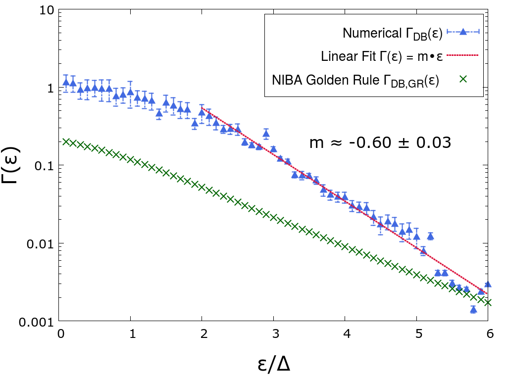
For increasing barrier heights, we expect the super-exchange rate to control the population decay if . The perturbative treatment leads to a characteristic algebraic dependence with , in contrast to the exponential one for sequential hopping. The results in Fig. 13 for moderate to large bridge energies verify the expected power law dependence with an exponent , close to the perturbative expectation.

Comparison with Master Equation Results
In case of weak system-reservoir couplings, the master equations build standard perturbative approaches to open system dynamics [1]. The corresponding time evolution equations for the reduced density matrix are formulated in terms of the eigenstates of the bare systems with the dissipator inducing transitions between these states. While these methods clearly fail for stronger couplings, it is nevertheless instructive to analyze their deficiencies in the context of rate dynamics.
Here, we use a standard master equation (ME) for which the dynamics of the diagonal elements of the reduced density matrix decouples from that of the off-diagonal elements. In the eigenstate representation of the Hamiltonian eq. (30), , one then has
| (44) |
where . The transition rates are obtained as
| (45) |
with and the thermal occupation . The stationary solution of (44) reproduces the Gibbs state distribution with partition function . The dynamics of the off-diagonal elements can simply be solved
| (46) |
with decay rates
| (47) | |||||
Now, the population dynamics in the site representation is obtained from this time evolution by a simple unitary transformation yielding
| (48) |
Note that the site populations are also determined by the dynamics of the off-diagonal elements in the eigenstate representation; the respective timescales are entirely determined through eqs. (45), (47).


We start in Fig. 14 with the population dynamics in the coherent regime (weak coupling). While the master results capture the transient oscillatory pattern qualitatively correctly, quantitatively deviations are clearly apparent. The time scales for relaxation towards thermal equilibrium are quite different with the master results approaching a steady state on a much faster time scale than the TCBD data. This may be attributed to the relatively low temperature which is beyond the validity of the Born-Markov approximation on which the master equation is based. The steady state values for the populations are basically identical though. Discrepancies in the relaxation dynamics substantially increase for stronger system bath couplings, see Fig. 15, when the dynamics tends to become a simple decay in time. Based on the rate extraction method presented before, we can now also extract respective rates from the master equation dynamics providing us with corresponding rates and super-exchange tunneling . The sequential transfer rate in Fig. 16 reveals indeed an exponential decay , however, with substantial deviations from the thermal value . The situation for the super-exchange rates is even worse as the extracted rates lack a physical interpretation, see Fig. 17: The numerical saturate for growing bridge energies to eventually become independent of at all, in contradiction to an algebraic decay.


This result is not so astonishing since, as already mentioned above, the parameter domain where incoherent population dynamics exhibits substantial quantum effects lies at the very edge or even beyond the range of validity of master equations. What is interesting nevertheless, is the fact that the explicit time scales appearing in eq. (48) can be directly related to the extracted super-exchange rate . This is shown in Fig. 18. It turns out that indeed non-local processes in the site representation (super-exchange) correspond to the decay rate of off-diagonal elements of the density matrix in the energy representation implying that already for moderate bridge energies .

VI Conclusion
In this work we combined a stochastic description of open quantum dynamics with projection operator techniques to improve convergence properties. While the general strategy has been outlined recently by one of us [39], we here restricted ourselves to a broad class of systems for which the dephasing time is finite. For the dynamics of the coherences of the reduced density one then keeps track of bath induced retardation effects only within a time window which must be tuned until convergence is achieved. While for with being the full propagation time one recovers the full stochastic description, the new TCBD is superior if is sufficiently shorter than . In parameter space this applies to the non-perturbative regime beyond weak coupling, a domain which is notoriously difficult to tackle, particularly at low temperatures.
The new TCBD scheme captures systems with continuous degree of freedom for arbitrary coupling strengths and to those with discrete Hilbert space up to moderate couplings. It allows to approach also the long time domain, where equilibration sets in. For two- and three-level systems we have shown explicitly that the new scheme covers both coherent as well as incoherent dynamics. In this latter regime the method is sufficiently accurate to extract quantum relaxation rates in the long time limit. It now allows for a variety of applications, for example, the dynamics of nonlinear quantum oscillators also in presence of external time dependent driving, the heat transfer through spin chains, or the quantum dynamics under optimal control protocols.
Acknowledgements.
This work was supported by the federal state of Baden-Wuerttemberg through a doctoral scholarship under the postgraduate scholarships act (LGFG) and by the DFG through the SFB/TRR 21.References
- [1] H. -P. Breuer and F. Petruccione, The Theory of Open Quantum Systems, Oxford University Press, Oxford, 2002.
- [2] U. Weiss, Quantum dissipative systems, 4th ed., World Scientific, Singapore, 2012.
- [3] A. O. Caldeira and A. J. Leggett, Phys. Rev. Lett. 46, 211 (1981); Ann. Phys. (N.Y.) 149, 374 (1983).
- [4] R. Zwanzig, Nonequilibrium Statistical Mechanics, Oxford University Press, Oxford, UK, 2001.
- [5] C. Gardiner, Stochastic Methods: A Handbook for the Natural and Social Sciences, 4th ed., Springer Series In Synergetics, Berlin, 2009.
- [6] A. Kossakowski, Rep. Math. Phys. 3, 247 (1972).
- [7] A. Kossakowski, Bull. Acad. Pol. Sci., Ser. Math. Astron. Phys. 20, 1021 (1972).
- [8] V. Gorini, A. Kossakowski and E. C. G. Sudarshan, J. Math. Phys. 17, 821 (1976).
- [9] G. Lindblad, Commun. Math. Phys. 48, 119 (1976).
- [10] J. Piilo, S. Maniscalco, K. Härkönen and K. -A. Suominen, Phys. Rev. Lett 100, 180402 (2008).
- [11] R. Vasile, S. Maniscalco, M. G. A. Paris, H. -P. Breuer and J. Piilo, Phys. Rev. A 84, 052118 (2011).
- [12] M. M. Wolf, J. Eisert, T. S. Cubitt, and J. I. Cirac Phys. Rev. Lett. 101, 150402 (2008).
- [13] H. -P. Breuer, E. -M. Laine and J. Piilo, Phys. Rev. Lett. 103, 210401 (2009).
- [14] D. Chruscinski and S. Maniscalco, Phys. Rev. Lett. 112, 120404 (2014).
- [15] A. Rivas, S. F. Huelga and M. B. Plenio, Rep. Prog. Phys. 77, 9 (2014).
- [16] F. W. J. Hekking and J. P. Pekola, Phys. Rev. Lett. 111, 093602 (2013).
- [17] J. Dalibard, Y. Castin and K. Mølmer, Phys. Rev. Lett. 68, 580 (1992).
- [18] R. Dum, P. Zoller and H. Ritsch, Phys. Rev. A 45, 4879 (1992).
- [19] H. -P. Breuer and F. Petruccione, Phys. Rev. E 52, 428 (1995).
- [20] N. Gisin and I. C. Percival, J. Phys. A 25, 5677 (1992).
- [21] I. Percival, Quantum State Diffusion, Cambridge University Press, Cambridge, 1998.
- [22] See e.g.: F. B. Anders, R. Bulla, and M. Vojta, Phys. Rev. Lett. 98, 210402 (2007).
- [23] See e.g.: H. Wang and M. Thoss, Chem. Phys. 370, 78 (2010).
- [24] See e.g.: J. Prior, A. W. Chin, S. F. Huelga and M. B. Plenio, Phys. Rev. Lett. 105, 050404 (2010).
- [25] R. P. Feynman and F. L. Vernon, Ann. Phys. 24, 118 (1963).
- [26] H. Grabert, P. Schramm and G. -L. Ingold, Phys. Rep. 168, 115 (1988).
- [27] R. Egger and C. H. Mak, Phys. Rev. B 50, 15210 (1994).
- [28] L. Mühlbacher and J. Ankerhold, J. Chem. Phys. 122, 184715 (2005).
- [29] D. Kast and J. Ankerhold, Phys. Rev. Lett. 110, 010402 (2013).
- [30] D. E. Makarov and N. Makri, Chem. Phys. Lett. 221, 482 (1994).
- [31] A. Ishizaki and Y. Tanimura, J. Phys. Soc. Jpn. 74, 3131 (2005).
- [32] L. Diosi and W. T. Strunz, Phys. Rev. Lett. A 235, 569 (1997).
- [33] J. T. Stockburger and H. Grabert, Phys. Rev. Lett. 88, 170407 (2002).
- [34] J. Shao, J. Chem. Phys. 120, 5053 (2004).
- [35] J. T. Stockburger, J. Chem. Phys. 296, 159169 (2004).
- [36] H. Imai, Y. Ohtsuki, H. Kono, J. Chem. Phys. 446, 134141 (2015).
- [37] R. Schmidt, A. Negretti, J. Ankerhold, T. Calarco and J. T. Stockburger, Phys. Rev. Lett. 107, 130404 (2011).
- [38] C. H. Mak and D. Chandler, Phys. Rev. A 41, 5709(R) (1990).
- [39] J. T. Stockburger, Europhys. Lett. 115, 40010 (2016).
- [40] S. Nakajima, Progr. Theor. Phys. 20, (1958).
- [41] R. Zwanzig, J. Chem. Phys. 33, (1960).
- [42] H. B. Callen, T. A. Welton, Phys. Rev. 83, 34 (1951).
- [43] A. O. Caldeira and A. J. Leggett, Physica A 121, 587616 (1983).
- [44] J. T. Stockburger and C.-H. Mak, J. Chem. Phys. 110, 4983 (1999).
- [45] J. T. Stockburger, Stochastic methods for the dynamics of open quantum systems, Habilitationsschrift, unpublished, Stuttgart, 2006.
- [46] J. T. Stockburger, Phys. Rev. E 59, R4709 (1999).
- [47] W. Koch, F. Großmann, J. T. Stockburger and J. Ankerhold, Phys. Rev. Lett. 100, 230402 (2008).
- [48] R. Schmidt, J. T. Stockburger and J. Ankerhold, Phys. Rev. A 88, 052321 (2013).
- [49] R. Schmidt, M. F. Carusela, J. P. Pekola, S. Suomela and J. Ankerhold, Phys. Rev. B 91, 224303 (2015).
- [50] J. T. Stockburger and T. Motz, Thermodynamic deficiencies of some simple Lindblad operators, arXiv: 1606.04326v1 (2016).
- [51] A. J. Leggett, S. Chakravarty, A. T. Dorsey, Matthew P. A. Fisher, Anupam Garg and W. Zwerger, Rev. Mod. Phys. 59, 1 (1987); ibid. 67, 725 (1995).
- [52] H. Dekker, Phys. Rev. A 35, 1436 (1987).
- [53] L. Mühlbacher, J. Ankerhold and C. Escher, J. Chem. Phys. 121, 12696 (2004).