Leptoquark Flavor Patterns & $B$ Decay Anomalies

Preprint: DO-TH 16/17

Gudrun Hiller Email: ghiller@physik.uni-dortmund.de Affiliation: Fakultät Physik, TU Dortmund, Otto-Hahn-Str.4, D-44221 Dortmund, Germany Dennis Loose Email: dennis.loose@udo.edu Affiliation: Fakultät Physik, TU Dortmund, Otto-Hahn-Str.4, D-44221 Dortmund, Germany Kay Schönwald Email: kay.schoenwald@udo.edu Affiliation: Fakultät Physik, TU Dortmund, Otto-Hahn-Str.4, D-44221 Dortmund, Germany

Abstract

Flavor symmetries that explain masses and mixings of the standard model fermions dictate flavor patterns for the couplings of scalar and vector leptoquarks to the standard model fermions. A generic feature is that couplings to $SU(2)$ -doublet leptons are suppressed at least by one spurion of the discrete non-abelian symmetry breaking, responsible for neutrino mixing, while couplings to charged lepton singlets can be order one. We obtain testable patterns including those that predominantly couple to a single lepton flavor, or two, or in a skewed way. They induce lepton non-universality, which we contrast to current anomalies in $B$ -decays. We find maximal effects in $R_{D}$ and $R_{D^{*}}$ at the level of $\sim$ 10 percent and few percent, respectively, while leptoquark effects in $R_{K^{(*)}}$ can reach order few $\times 10$ percent. Predictions for charm and kaon decays and $\mu-e$ conversion are worked out.

I Introduction

Generational structure and its manifestation through fermion masses and mixings is one of the key ingredients of the Standard Model (SM), however, the origin of flavor remains a puzzle. While quark flavor solely resides in the Yukawa couplings to the Higgs, flavor breaking in the lepton sector is even less clear-cut as neutrino masses could stem from a different mechanism.

Flavor symmetries explain the observed masses and mixings of the SM fermions, however, viable solutions are not unambiguous. Physics beyond the SM provides opportunities for new insights, as new couplings allow for different combinations of flavor symmetry breaking. A well-known example is the minimal supersymmetric SM. Here masses and mixings of scalar quarks and leptons are present which allow to probe also non-chiral combinations of matter bilinears [1].

Here we consider scalar and vector leptoquark extensions of the SM [2, 3]. Representations for $SU(3)_{C}\times SU(2)_{L}\times U(1)_{Y}$ and renormalizable couplings to SM fermions are given in Appendix A. We assume that proton decay is safe, note, however, to ensure this requires further model-building for some of the leptoquarks [4]. There are in total twelve different types of flavor-matrices that appear in leptoquark models with couplings to $SU(2)_{L}$ doublet quarks $Q$ and leptons $L$ , and $SU(2)_{L}$ singlet quarks $U,D$ and charged leptons $E$ , schematically,

\displaystyle Y_{AB},Y_{\bar{A}B}\,,\quad A=Q,U,D\,,\penalty\ \penalty\ B=L,E\,,

(1)

where rows and columns correspond to quarks and leptons, respectively. To simplify the discussion, in the following these couplings are denoted Yukawa matrices for both scalar and vector leptoquarks.

Table 1 shows for which leptoquark scenario which type of yukawa is present. Also indicated is by a checkmark which yukawa contributes at tree level to (semi-)leptonic flavor changing neutral current (FCNC) transitions in the down and up-quark sector. Contributions to charged currents, e.g., $b\to c\ell\nu$ in chirality-preserving four-fermion interactions, $\bar{Q}\gamma_{\mu}(\sigma^{a})Q\bar{L}\gamma^{\mu}(\sigma^{a})L$ [5] arise from $Y_{QL}$ , $Y_{\bar{Q}L}$ only. $\sigma^{a}$ denote the Pauli-matrices. $S_{1,2}$ and $V_{1,2}$ induce charged currents through a combination of their two couplings present, resulting in chirality-flipping operators.

$AB$	$QL$	$\bar{Q}L$	$UL$	$\bar{U}L$	$DL$	$\bar{D}L$	$QE$	$\bar{Q}E$	$UE$	$\bar{U}E$	$DE$	$\bar{D}E$
model	$S_{1,3}$	$V_{1,3}$	$\tilde{V}_{2}$	$S_{2}$	$V_{2}$	$\tilde{S}_{2}$	$V_{2}$	$S_{2}$	$S_{1}$	$\tilde{V}_{1}$	$\tilde{S}_{1}$	$V_{1}$
down-type FCNC	✓	✓	–	–	✓	✓	✓	✓	–	–	✓	✓
up-type FCNC	✓	✓	✓	✓	–	–	✓	✓	✓	✓	–	–

Table 1: Leptoquark couplings

Y_{AB}

and

Y_{\bar{A}B}

as they appear in various leptoquark models as well as in tree level down-type quark FCNCs and up-type quark FCNCs. Models

S_{1,2}

and

V_{1,2}

have two yukawas each.

Patterns based on a $U(1)_{\text{FN}}$ -Froggatt–Nielsen (FN) symmetry [6], combined with a non-abelian discrete symmetry, $A_{4}$ , have been worked out previously for leptoquarks coupling to lepton doublets [7, 8]. Here we provide further details and flavor patterns involving singlet leptons. The $U(1)_{\text{FN}}$ explains hierarchies in the quark sector and for the charged lepton masses, while non-abelian discrete subgroups of $SU(3)$ can accommodate neutrino mixing [9]. We stress that leptoquark extensions of the SM are special as they can access both quark and lepton flavor.

Leptoquark models have been considered recently in the context of lepton non-universality (LNU) and lepton flavor violating (LFV) observables in semileptonic $b\to s$ and $b\to c$ decays. While there is vast literature on leptoquark models addressing LNU in $B\to D^{(*)}\ell\nu$ decays, the leptonic flavor structure in these studies is either of an assumed, simple type such as third generation only, of within minimal flavor violation and variants thereof, or parametrical amended by experimental constraints [10, 11, 12, 13, 14, 15, 16, 17, 18, 19], and references therein. Our aim is here to close this gap and work out leptoquark effects based on flavor symmetries. For previous leptoquark studies regarding LNU in $B\to K\ell\ell$ decays, see, for instance, [21, 16, 22, 7, 12, 23, 24, 17, 15, 20, 18].

The plan of the paper is as follows: In Sections II and III we summarize the main model-building tools for obtaining flavor patterns for Yukawa matrices, and present patterns in Section III. In Section IV we work out phenomenological implications for $B\to D^{(*)}\ell\nu$ , $B\to K^{(*)}\ell\ell$ , rare charm and $K$ decays and $\mu-e$ conversion. We conclude in Section V. Auxiliary formulae and tables are given in Appendices A-D.

II Flavor Hierarchies

We discuss the hierarchical structure of the leptoquark couplings due to an $U(1)_{\text{FN}}$ which explains flavor in the quark sector and the masses of the charged leptons. To obtain mixing in the lepton sector we additionally invoke a discrete non-abelian symmetry, $A_{4}$ [25], discussed in Section III.

FN-charges $q$ for quarks and leptons are obtained in [26]; for instance, a realistic set is given by

\displaystyle q(\bar{Q})

\displaystyle=q(U)=(4,2,0)\,,\quad q(D)=(3,2,2)\,,\quad q(E)=(4,2,0)\,,\quad q(L)=0\,.

(2)

By choosing this as our benchmark, we assumed that the Higgs vacuum expectation values (VEVs) responsible for up- and down-quark masses are similar in size to cover a SM-like situation in which they are identical. In supersymmetric variants or multi-Higgs models with larger values of $\tan\beta$ , the Higgs VEV ratio, smaller values of $q(D)$ are possible. Corresponding effects in the lepton sector can be taken into account by adjusting the VEV of the non-abelian flavor symmetry breaking responsible for charged lepton masses.

The parametric suppression of the leptoquark yukawas in terms of powers of $\lambda\sim 0.2$ is then determined as

\displaystyle\left(Y_{AB}\right)_{ij}\sim\lambda^{|q(A_{i})+q(B_{j})|}\,,\quad\left(Y_{\bar{A}B}\right)_{ij}\sim\lambda^{|-q(A_{i})+q(B_{j})|}\,,

(3)

where we assumed that the leptoquarks are uncharged under the FN-symmetry. Allowing for a finite charge would rescale the overall size of the yukawas.

From Eq. (3) it is apparent that, unlike in the SM, charges from the quark sector can interfere with the ones from the lepton sector. In particular, with assignments Eq. (2) cancellations can arise for $QE,\bar{D}E$ and $\bar{U}E$ corresponding to the vector leptoquark scenarios $V_{2},V_{1}$ and $\tilde{V}_{1}$ , respectively. This causes the hierarchy expected from the quark masses to be inverted in these scenarios. For $\bar{Q}E,DE$ and $UE$ corresponding to the scalar leptoquark scenarios $S_{2},\tilde{S}_{1}$ and $S_{1}$ , respectively, the hierarchies will be stronger than from the quarks alone. If instead the singlet-lepton charges would be chosen with opposite sign to the quark ones, the effects would swap, that is, an inversion of hierarchies would occur for scalar and an increase of hierarchies for vector leptoquarks. Lepton-doublet scenarios would also be affected in models with $q(L)\neq 0$ . For $q(L)=0$ , $Y_{AL}=Y_{\bar{A}L}$ .

The breaking of the $U(1)_{\text{FN}}$ can lead to BSM scalars (flavons) in reach of present or future colliders, with corresponding phenomenology driven by the FN-charges, e.g., [27, 28]. Such analysis is interesting, however, beyond the scope of our paper, which focusses on leptoquark-induced BSM effects.

III Flavor selection with discrete symmetries

We employ the discrete symmetry $A_{4}\times Z_{3}$ to model the lepton mixing based on a modification [29] of the original model [25], which introduces an additional field to account for a non-vanishing value of $\theta_{13}$ . Table 2 summarizes the charge assignments of the leptons and the flavon fields, adopted from [7]. The FN-spurion is uncharged under $A_{4}\times Z_{3}$ .

	$L$	$e_{\text{R}}$	$\mu_{\text{R}}$	$\tau_{\text{R}}$	$\phi_{\ell}$	$\phi_{\nu}$	$\xi$	$\xi^{\prime}$
$A_{4}$	3	1	$1^{\prime}$	$1^{\prime\prime}$	3	3	1	$1^{\prime}$
$Z_{3}$	1	1	1	1	0	2	2	2

Table 2: Non-trivial

A_{4}\times Z_{3}

charge assignments. For leptoquarks, see text.

The VEVs of the flavons are given as $\langle\phi_{\ell}\rangle/\Lambda=c_{\ell}(1,0,0)$ , $\langle\phi_{\nu}\rangle/\Lambda=c_{\nu}(1,1,1)$ and $\langle\xi^{(\prime)}\rangle/\Lambda=\kappa^{(\prime)}$ , where $\Lambda$ denotes a new physics scale related to $A_{4}$ -breaking. The values of the VEVs are, in general, model-dependent. Typically, $c_{\ell,\nu},\kappa^{(\prime)}\lesssim\lambda^{\rm few}$ to explain charged lepton and neutrino parameters. Here and in the following we use the term “VEV” for $c_{\ell,\nu},\kappa^{(\prime)}$ as well. While the latter are dimensionless numbers it should be clear that they do not correspond to renormalizable couplings of the full Lagrangian.

For completeness, we briefly summarize the multiplication rules for $A_{4}$ . For further information on the basis and group theory of $A_{4}$ see [30]. The group has three singlet representations $1$ , $1^{\prime}$ , and $1^{\prime\prime}$ which form a $Z_{3}$ subgroup with the usual multiplication rules. Additionally, $A_{4}$ has a triplet representation. Denoting two triplets as $A=(a_{1},a_{2},a_{3})$ and $B=(b_{1},b_{2},b_{3})$ the product reads

$\displaystyle\left(AB\right)_{1\phantom{{}^{\prime\prime}}}$	$\displaystyle=a_{1}b_{1}+a_{2}b_{3}+a_{3}b_{2}\sim 1,$	(4)
$\displaystyle\left(AB\right)_{1^{\prime}\phantom{{}^{\prime}}}$	$\displaystyle=a_{1}b_{2}+a_{2}b_{1}+a_{3}b_{3}\sim 1^{\prime},$	(5)
$\displaystyle\left(AB\right)_{1^{\prime\prime}}$	$\displaystyle=a_{1}b_{3}+a_{2}b_{2}+a_{3}b_{1}\sim 1^{\prime\prime}$	(6)

and

\displaystyle\left(AB\right)_{s}

\displaystyle=\frac{1}{3}\begin{pmatrix}2a_{1}b_{1}-a_{2}b_{3}-a_{3}b_{2}\\ 2a_{3}b_{3}-a_{1}b_{2}-a_{2}b_{1}\\ 2a_{2}b_{2}-a_{3}b_{1}-a_{1}b_{3}\end{pmatrix},

\displaystyle\left(AB\right)_{a}

\displaystyle=\frac{1}{2}\begin{pmatrix}a_{2}b_{3}-a_{3}b_{2}\\ a_{1}b_{2}-a_{2}b_{1}\\ a_{3}b_{1}-a_{1}b_{3}\end{pmatrix},

(7)

with a symmetric ( $s$ ) and an antisymmetric ( $a$ ) triplet.

Firstly, all quarks are considered $A_{4}$ singlets (Section III.1). In Section III.2 we discuss patterns for individual quark generations in non-trivial singlet-representations of $A_{4}$ .

III.1 Quarks trivial under $A_{4}$

III.1.1 Flavor patterns

If all quarks have a trivial $A_{4}$ -charge and identical $Z_{3}$ -charges, one needs to distinguish only between the couplings to right-handed leptons $Y_{AE}(Y_{\bar{A}E})$ and to left-handed leptons $Y_{AL}(Y_{\bar{A}L})$ . The column structure of the patterns is governed by the $A_{4}$ and $Z_{3}$ -charges of the leptoquark. The $A_{4}$ -charge determines to which lepton generation(s) the leptoquark can couple, while the $Z_{3}$ -charge selects the flavon field that mediates the coupling. We denote the leptoquarks $S_{i}^{\dagger},V_{i}^{\dagger}$ generically by $\Delta$ and the charge assignments by $[\Delta]_{A_{4}}$ etc.

For the left-handed couplings the crucial flavons are the $A_{4}$ -triplets $\phi_{\ell}$ and $\phi_{\nu}$ , which produce patterns that either isolate a single lepton generation or couple equally to all generations [7].

For the right-handed leptons, terms of the form $A\Delta E$ are $Z_{3}$ -invariant without any additional flavon insertion for $[\Delta]_{Z_{3}}=2$ . (Here and in the following, as in Eq. (1), $A$ ( $B$ ) generically denotes quark (lepton) fields.) In this case one isolates a single lepton generation, depending on the leptoquark’s $A_{4}$ -representation. Additionally, and in contrast to the respective pattern for the left-handed coupling, the isolated column is suppressed by powers of $\lambda$ due to the FN-charges of the right-handed leptons. For $[\Delta]_{Z_{3}}=0$ one additional flavon, $\xi$ or $\xi^{\prime}$ , is needed. Since the latter have identical $Z_{3}$ -charge but transform under different singlet representations of $A_{4}$ , two lepton generations are isolated.

To summarize these findings we introduce the following lepton flavor isolation textures

\displaystyle k_{e}=\begin{pmatrix}*&0&0\\ *&0&0\\ *&0&0\end{pmatrix},\quad k_{\mu}=\begin{pmatrix}0&*&0\\ 0&*&0\\ 0&*&0\end{pmatrix},\quad k_{\tau}=\begin{pmatrix}0&0&*\\ 0&0&*\\ 0&0&*\end{pmatrix}\,,

(8)

from which all patterns can be constructed. Here, “ $*$ ” denote non-zero entries whose parametric flavor dependence is given by the $U(1)_{\text{FN}}$ . Table 3 shows the resulting patterns for the Yukawa matrices $Y_{AL}(Y_{\bar{A}L})$ and $Y_{AE}(Y_{\bar{A}E})$ as linear combinations of the $k_{\ell}$ -matrices, $\ell=e,\mu,\tau$ .

	$k_{e}$	$k_{\mu}$	$k_{\tau}$	$\left[\Delta\right]_{A_{4}}$	$\left[A\Delta B\right]_{Z_{3}}$	name
$Y_{AL}(Y_{\bar{A}L})$	$c_{\ell}$	$0$	$0$	$1\phantom{{}^{\prime\prime}}$	$0$	$L_{e}$
	$0$	$c_{\ell}$	$0$	$1^{\prime\prime}$		$L_{\mu}$
	$0$	$0$	$c_{\ell}$	$1^{\prime}\phantom{{}^{\prime}}$		$L_{\tau}$
	$c_{\nu}$	$c_{\nu}$	$c_{\nu}$	$1$ , $1^{\prime}$ , $1^{\prime\prime}$	$1$	$L_{d}$
	$c_{\nu}\kappa$	$c_{\nu}\kappa$	$c_{\nu}\kappa$	$1$ , $1^{\prime}$ , $1^{\prime\prime}$	$2$	$L_{d^{\prime}}$
$Y_{AE}(Y_{\bar{A}E})$	$1$	$0$	$0$	$1\phantom{{}^{\prime\prime}}$	$0$	$R_{e}$
	$0$	$1$	$0$	$1^{\prime\prime}$		$R_{\mu}$
	$0$	$0$	1	$1^{\prime}\phantom{{}^{\prime}}$		$R_{\tau}$
	$\kappa$	$0$	$\kappa^{\prime}$	$1\phantom{{}^{\prime\prime}}$	$1$	$R_{e\tau}$
	$\kappa^{\prime}$	$\kappa$	$0$	$1^{\prime\prime}$		$R_{e\mu}$
	$0$	$\kappa^{\prime}$	$\kappa$	$1^{\prime}\phantom{{}^{\prime}}$		$R_{\mu\tau}$
	$\kappa^{\prime 2}$	$\kappa^{\prime 2}$	$\kappa^{\prime 2}$	$1$ , $1^{\prime}$ , $1^{\prime\prime}$	$2$	$R_{d}$

Table 3: Patterns for the Yukawa matrices of left-handed (upper part) and right-handed (lower part) leptons for leptoquarks in singlet representations of

A_{4}

. Additional FN-factors apply and are given in Eq. (3).

For instance, the $R_{e\mu}$ pattern corresponds to $\kappa^{\prime}k_{e}+\kappa k_{\mu}$ amended by FN-factors that depend on the leptoquark scenario and can be taken from Eqs. (3) and (2)

\displaystyle R_{e\mu}(UE)=\begin{pmatrix}\kappa^{\prime}\lambda^{8}&\kappa\lambda^{6}&0\\ \kappa^{\prime}\lambda^{6}&\kappa\lambda^{4}&0\\ \kappa^{\prime}\lambda^{4}&\kappa\lambda^{2}&0\end{pmatrix}\,,\penalty\ R_{e\mu}(\bar{U}E)=\begin{pmatrix}\kappa^{\prime}\lambda^{0}&\kappa\lambda^{2}&0\\ \kappa^{\prime}\lambda^{2}&\kappa\lambda^{0}&0\\ \kappa^{\prime}\lambda^{4}&\kappa\lambda^{2}&0\end{pmatrix}\,.

(9)

It is manifest from these patterns that generational hierarchies can be inverted relative to the ones of the fermion mass terms. Neglecting terms of order $\lambda^{2}$ the pattern $R_{e\mu}(\bar{U}E)$ , which can appear in the $\tilde{V}_{1}$ scenario, closely resembles patterns leading to sizable LFV in rare charm decays [8]. Contributions with $\left[A\Delta B\right]_{Z_{3}}=2$ arise at second order in the $A_{4}$ -flavon expansion, and yield democratic patterns, $L_{d^{\prime}}$ and $R_{d}$ , see Table 3.

For the leptoquarks $S_{1},S_{2},V_{1}$ and $V_{2}$ both left- and right-handed couplings can be present simultaneously. Since the lepton and quark mass terms must be $Z_{3}$ -invariant, both interaction terms of the respective leptoquark must have identical $Z_{3}$ -charge

[QL\Delta]_{Z_{3}}=[UE\Delta]_{Z_{3}},\ [\bar{U}L\Delta]_{Z_{3}}=[\bar{Q}E\Delta]_{Z_{3}},\ [\bar{Q}L\Delta]_{Z_{3}}=[\bar{D}E\Delta]_{Z_{3}},\ [DL\Delta]_{Z_{3}}=[QE\Delta]_{Z_{3}}

(10)

and identical $A_{4}$ -charge of the $\Delta$ . Possible correlations can be read-off from Table 3. For instance, $\left[A\Delta B\right]_{Z_{3}}=0$ gives $L_{\ell}$ and $R_{\ell}$ , with the joint lepton flavor $\ell$ fixed by $\left[\Delta\right]_{A_{4}}$ . Note, that there is an overall hierarchy between the left-handed couplings, which go with $c_{\ell}$ , and the right-handed ones, which are order one. Another possibility is $\left[A\Delta B\right]_{Z_{3}}=1$ , which induces $L_{d}$ together with one of the $R_{\ell\ell^{\prime}}$ ones, where the selection of leptons is again fixed by $\left[\Delta\right]_{A_{4}}$ . For $c_{\nu}\ll\kappa,\kappa^{\prime}$ the democratic and phenomenologically dangerous pattern can be suppressed relative to the lepton singlet couplings.

Quite generally, and beyond the explicit $A_{4}\times Z_{3}$ model, the flavon VEV suppression in leptoquark couplings to lepton doublets cannot be avoided, once the three generations of doublets are in a triplet representation of the non-abelian group in order to give the Pontecorvo-Maki-Nakagawa-Sakata (PMNS)-matrix. This feature is of course manifest [7] in the $A_{4}\times Z_{4}$ model [31, 29]. Requiring invariance of the term $A\Delta L$ one therefore needs an insertion of a triplet flavon VEV. The other alternative would be to make the leptoquark a triplet, which leads to a democratic pattern and does not give rise to LNU. Note, in see-saw models, terms with right-handed neutrinos, which are triplets of $A_{4}$ and carry $Z_{2}=2$ [31] result in VEV-suppressed, democratic patterns.

III.1.2 Mass basis rotation

We consider modifications of the patterns derived in the flavor basis from changing to the mass basis. The corresponding transformations of the fermion fields by the unitary matrices $U,V$ read

$\displaystyle u_{\text{L}}$	$\displaystyle\to V_{u}u_{\text{L}}\,,$	$\displaystyle d_{\text{L}}$	$\displaystyle\to V_{d}d_{\text{L}}\,,$	(11)
$\displaystyle u_{\text{R}}$	$\displaystyle\to U_{U}u_{\text{R}}\,,$	$\displaystyle d_{\text{R}}$	$\displaystyle\to U_{D}d_{\text{R}}\,,$	(12)
$\displaystyle\ell_{\text{L}}$	$\displaystyle\to U_{L}\ell_{\text{L}}\,,$	$\displaystyle\nu_{\text{L}}$	$\displaystyle\to U_{\nu}\nu_{\text{L}}\,,$	(13)
$\displaystyle\ell_{\text{R}}$	$\displaystyle\to U_{E}\ell_{\text{R}}\,,$			(14)

from which the Cabibbo-Kobayashi-Maskawa (CKM) and PMNS mixing matrices are obtained as

\displaystyle V_{\text{CKM}}=V_{u}^{\dagger}V_{d}\,,\quad V_{\text{PMNS}}=U_{L}^{\dagger}U_{\nu}\,.

(15)

In leptoquark models also other combinations become physical. In particular, the leptoquark yukawas transform as

\displaystyle Y_{AB}\to U_{A}^{T}Y_{AB}U_{B}\,,\quad Y_{\bar{A}B}\to U_{A}^{\dagger}Y_{\bar{A}B}U_{B}\,.

(16)

Quark rotations therefore only mix rows, whereas lepton rotations only mix columns.

The parametric dependence of the rotation matrices in the quark sector can be obtained by perturbative diagonalization [32] as ¹¹ 1 For the charges given in Eq. (2) some tuning has to be done to recover $V_{us}$ .

$\displaystyle\left(V_{u}\right)_{ij}\sim\left(V_{d}\right)_{ij}$	$\displaystyle\sim\lambda^{\|q(Q_{i})_{-}q(Q_{j})\|}\,,$
$\displaystyle\left(U_{U}\right)_{ij}$	$\displaystyle\sim\lambda^{\|q(U_{i})-q(U_{j})\|}\,,$	(17)
$\displaystyle\left(U_{D}\right)_{ij}$	$\displaystyle\sim\lambda^{\|q(D_{i})-q(D_{j})\|}\,.$

The resulting mixing of the rows does not spoil the patterns as the hierarchical suppression of the leptoquark yukawas stays parametrically intact. Note, that this does not hold true anymore for quarks charged non-trivially under $A_{4}$ , as discussed in Section III.2.

Since the transformations $U,V$ are unitary and neutrinos are inclusively reconstructed in collider experiments, the rotation $V_{\nu}$ has no impact on such observables. Furthermore, in the $A_{4}\times Z_{3}$ framework considered in this work, the charged lepton Yukawa matrix $Y_{\ell}$ is already diagonal at leading order. However, higher order flavon insertions can induce non-diagonal entries in $Y_{\ell}$ [33]. We discuss this in the next section together with other higher order effects.

III.1.3 Higher order flavon corrections

It is easy to compute $Y_{\ell}$ including next-to leading order corrections

Y_{\ell}\sim c_{\ell}\left[\begin{pmatrix}\lambda^{4}&0&0\\ 0&\lambda^{2}&0\\ 0&0&1\end{pmatrix}+\delta\begin{pmatrix}\lambda^{4}&\lambda^{2}&1\\ \lambda^{4}&\lambda^{2}&1\\ \lambda^{4}&\lambda^{2}&1\end{pmatrix}\right]\sim c_{\ell}\begin{pmatrix}\lambda^{4}&\delta\lambda^{2}&\delta\\ \delta\lambda^{4}&\lambda^{2}&\delta\\ \delta\lambda^{4}&\delta\lambda^{2}&1\end{pmatrix}\,,

(18)

from which the rotation matrices follow as, using perturbative diagonalization [32],

\displaystyle U_{L}\sim\begin{pmatrix}1&\delta&\delta\\ \delta&1&\delta\\ \delta&\delta&1\end{pmatrix}\,,\quad U_{E}\sim\begin{pmatrix}1&\delta\lambda^{2}&\delta\lambda^{4}\\ \delta\lambda^{2}&1&\delta\lambda^{2}\\ \delta\lambda^{4}&\delta\lambda^{2}&1\end{pmatrix}\,.

(19)

Here, we introduced a parameter $\delta<1$ , of the order $({\rm VEV})^{2}$ ,

\delta\sim\text{max}\left(\frac{c_{\nu}^{3}}{c_{\ell}},\frac{c_{\nu}\kappa^{2}}{c_{\ell}},\frac{c_{\nu}\kappa\kappa^{\prime}}{c_{\ell}},\frac{c_{\nu}\kappa^{\prime 2}}{c_{\ell}}\right)\,.

(20)

The effect of transforming the left-handed charged leptons is therefore ${\cal{O}}(\delta)$ , at second relative order in the flavon expansion and modifies $Y_{AL,\bar{A}L}$ . This implies, for instance, for the tau-isolation pattern

\displaystyle L_{\tau}(UL,\bar{U}L,QL,\bar{Q}L)\to c_{\ell}\begin{pmatrix}\delta\lambda^{4}&\delta\lambda^{4}&\lambda^{4}\\ \delta\lambda^{2}&\delta\lambda^{2}&\lambda^{2}\\ \delta&\delta&\lambda^{0}\end{pmatrix}\,.

(21)

Rotations stemming from the right-handed leptons contribute at higher orders in $\lambda$ . E.g., this effect modifies single and double lepton isolation patterns in $Y_{AE,\bar{A}E}$ such as those given in Eq. (9)

\displaystyle R_{e\mu}(\bar{U}E)\to\begin{pmatrix}\kappa^{\prime}\lambda^{0}&\kappa\lambda^{2}&\delta\lambda^{4}(\kappa+\kappa^{\prime})\\ \kappa^{\prime}\lambda^{2}&\kappa\lambda^{0}&\delta\lambda^{2}\kappa\\ \kappa^{\prime}\lambda^{4}&\kappa\lambda^{2}&\delta\lambda^{4}\kappa\end{pmatrix}\,.

(22)

For the $R_{\tau}$ -pattern mass rotation effects amount to

\displaystyle R_{\tau}(UE,\bar{U}E,QE,\bar{Q}E)\to\begin{pmatrix}\delta\lambda^{8}&\delta\lambda^{6}&\lambda^{4}\\ \delta\lambda^{6}&\delta\lambda^{4}&\lambda^{2}\\ \delta\lambda^{4}&\delta\lambda^{2}&\lambda^{0}\end{pmatrix}\,,\quad R_{\tau}(DE,\bar{D}E)\to\begin{pmatrix}\delta\lambda^{7}&\delta\lambda^{5}&\lambda^{3}\\ \delta\lambda^{6}&\delta\lambda^{4}&\lambda^{2}\\ \delta\lambda^{6}&\delta\lambda^{4}&\lambda^{2}\end{pmatrix}\,.

(23)

The patterns given in Table 3 receive in addition direct contributions from higher order flavon insertions. The single lepton generation isolating patterns with coupling to left-handed fermions, $L_{\ell}$ , receive corrections from replacing $\phi_{\ell}$ with $\phi_{\nu}$ plus two additional $A_{4}$ -singlet flavons or two insertions of $\phi_{\nu}$ . These contributions are $\mathcal{O}(c_{\nu}^{3}/c_{\ell})$ and $\mathcal{O}(c_{\nu}\kappa^{(\prime)2}/c_{\ell})$ , respectively, and universal for all entries modulo the FN-charges [7]. In terms of $\delta$ introduced before these higher order effects amount to the same as what we got from the mass basis rotation, Eq. (21). The democratic pattern $L_{d}$ is subject to next-to leading order corrections from $\phi_{\nu}\to\phi_{\ell}$ plus one additional $A_{4}$ -singlet. However, because of the unknown $\mathcal{O}(1)$ coefficients, these corrections are immaterial.

The explicit higher order flavon corrections to the patterns of right-handed leptons arise universally for each entry at third order: two times $\phi_{\nu}$ plus one singlet flavon or three singlet flavons. Denoting $\delta^{\prime}={\cal{O}}{(\rm VEV}^{3})$ , for $R_{\tau}$ ,

\displaystyle R_{\tau}(UE,\bar{Q}E)\!\to\!\!\begin{pmatrix}\delta^{\prime}\lambda^{8}&\delta^{\prime}\lambda^{6}&\lambda^{4}\\ \delta^{\prime}\lambda^{6}&\delta^{\prime}\lambda^{4}&\lambda^{2}\\ \delta^{\prime}\lambda^{4}&\delta^{\prime}\lambda^{2}&\lambda^{0}\end{pmatrix}\!,R_{\tau}(\bar{U}E,QE)\!\to\!\!\begin{pmatrix}\delta^{\prime}\lambda^{0}&\delta^{\prime}\lambda^{2}&\lambda^{4}\\ \delta^{\prime}\lambda^{2}&\delta^{\prime}\lambda^{0}&\lambda^{2}\\ \delta^{\prime}\lambda^{4}&\delta^{\prime}\lambda^{2}&\lambda^{0}\end{pmatrix}\!,R_{\tau}(\bar{D}E)\!\to\!\!\begin{pmatrix}\delta^{\prime}\lambda&\delta^{\prime}\lambda&\lambda^{3}\\ \delta^{\prime}\lambda^{2}&\delta^{\prime}\lambda^{0}&\lambda^{2}\\ \delta^{\prime}\lambda^{2}&\delta^{\prime}\lambda^{0}&\lambda^{2}\end{pmatrix}\!.

(24)

If there are cancellations between the FN charges of the quarks and leptons, these corrections can be larger than the mass rotation effect Eq. (23). For phenomenology one therefore has to take the maximum of each entry of Eq. (23) and (24). Similarly, for the double lepton isolation patterns

\displaystyle R_{e\mu}(\bar{U}E,\bar{Q}E)\to\begin{pmatrix}\kappa^{\prime}\lambda^{0}&\kappa\lambda^{2}&\delta^{\prime\prime}\lambda^{4}\\ \kappa^{\prime}\lambda^{2}&\kappa\lambda^{0}&\delta^{\prime\prime}\lambda^{2}\\ \kappa^{\prime}\lambda^{4}&\kappa\lambda^{2}&\delta^{\prime\prime}\lambda^{0}\end{pmatrix}\,,

(25)

where $\delta^{\prime\prime}={\cal{O}}{(\rm VEV}^{4})$ .

III.2 Quarks non-trivial under $A_{4}$

Single quarks in a non-trivial $A_{4}\times Z_{3}$ -representation allows to construct further flavor patterns for the leptoquarks. In Ref. [7] this has been discussed for $A_{4}\times Z_{4}$ models. Here, to formally restore $A_{4}\times Z_{3}$ -invariance of the SM yukawa terms of the quarks insertions of $\xi^{\prime}$ are necessary. In order to not destroy the quark masses and mixings, the $A_{4}$ -VEV suppression $\kappa^{\prime}\sim\lambda^{m}$ needs to be compensated by a corresponding change in FN-charge. Additionally, the $Z_{3}$ charge of the inserted flavon fields has to be cancelled. The following choices leave the SM Yukawa matrices of the quarks intact:

\displaystyle\left[A_{i}\right]_{A_{4}}

\displaystyle\to 1^{\prime\prime},\quad\left[A_{i}\right]_{Z_{3}}\to 1,\quad q(A_{i})\to q(A_{i})-m\,,

(26)

or, with two insertions,

\displaystyle\left[A_{i}\right]_{A_{4}}

\displaystyle\to 1^{\prime},\quad\left[A_{i}\right]_{Z_{3}}\to 2,\quad q(A_{i})\to q(A_{i})-2m\,.

(27)

Here, $A$ can be any of the quark fields $\bar{Q},U,D$ of first or second generation, $i=1,2$ . For the third generation this leads to a suppression of third generation yukawas.

The different charges for one generation of quarks lead to a mixing of rows between patterns characterized by different $\left[A\Delta B\right]_{Z_{3}}$ and $\left[\Delta\right]_{A_{4}}$ and a modified hierarchy in the entries “ $*$ ” of the lepton flavor isolating textures, $k_{\ell}$ . If the quark generations $j\neq i$ are trivially charged and couple to the pattern characterized by

\displaystyle\left[A\Delta B\right]_{Z_{3}}

\displaystyle=a\,,\quad[\Delta]_{A_{4}}\,,

(28)

see also Table 3, then the $i$ th row corresponding to the non-trivially charged quark is given by the pattern with

\displaystyle\left[A\Delta B\right]_{Z_{3}}

\displaystyle=\begin{cases}(a+1)\text{mod}\ 3\text{\quad for one insertion}\\ (a+2)\text{mod}\ 3\text{\quad for two insertions}\end{cases},

(29)

and the total $A_{4}$ -charge $[A\Delta]_{A_{4}}$ of the quark and the leptoquark. Note that since the FN-charge of quarks has been changed, corresponding mass basis rotations Eq. (17) do matter.

Choosing $\left[\bar{Q}_{2}\right]_{A_{4}}=\left[\Delta\right]_{A_{4}}=1^{\prime\prime}$ , that is, $a=0$ and $m=2$ gives a modification of the $\mu$ -isolation pattern, as

\displaystyle\tilde{L}_{\mu}(QL)

\displaystyle=\begin{pmatrix}0&c_{\ell}\lambda^{4}&0\\ c_{\nu}\kappa&c_{\nu}\kappa&c_{\nu}\kappa\\ 0&c_{\ell}\lambda^{0}&0\end{pmatrix},\quad\tilde{L}_{\mu}(\bar{Q}L)=\begin{pmatrix}0&c_{\ell}\lambda^{4}&0\\ c_{\nu}&c_{\nu}&c_{\nu}\\ 0&c_{\ell}\lambda^{0}&0\end{pmatrix},

(30)

where for $QL$ the second row has $\left[A\Delta B\right]_{Z_{3}}=2$ and correspondingly couples to $L_{d^{\prime}}$ and for $\bar{Q}L$ the second row has $\left[A\Delta B\right]_{Z_{3}}=1$ and correspondingly couples to $L_{d}$ . Including mass basis corrections

\displaystyle\tilde{L}_{\mu}(QL)\!\!\to\!\!\begin{pmatrix}c_{\nu}\kappa\lambda^{2}&c_{\ell}\lambda^{4}+c_{\nu}\kappa\lambda^{2}&c_{\nu}\kappa\lambda^{2}\\ c_{\nu}\kappa&c_{\ell}\lambda^{2}+c_{\nu}\kappa&c_{\nu}\kappa\\ c_{\ell}\delta+c_{\nu}\kappa\lambda^{2}&c_{\ell}&c_{\ell}\delta+c_{\nu}\kappa\lambda^{2}\end{pmatrix}\,,\tilde{L}_{\mu}(\bar{Q}L)\!\!\to\!\!\begin{pmatrix}c_{\nu}\lambda^{2}&c_{\nu}\lambda^{2}&c_{\nu}\lambda^{2}\\ c_{\nu}&c_{\ell}\lambda^{2}+c_{\nu}&c_{\nu}\\ \ c_{\ell}\delta+c_{\nu}\lambda^{2}&c_{\ell}&c_{\ell}\delta+c_{\nu}\lambda^{2}\end{pmatrix}\,,

(31)

where we note that due to Eq. (2) the FN-suppression of the first row is $\lambda^{2}$ . The FN-suppression of the second row present in $L_{\mu}$ is in $\tilde{L}_{\mu}$ turned into a VEV-suppression. The $\tilde{L}_{\mu}$ - patterns are relevant for $b\to s\mu\mu$ processes. Similarly, modifications of $\tau$ -isolation patterns can be obtained for $\left[\bar{Q}_{2}\right]_{A_{4}}=1^{\prime\prime}$ , $\left[\bar{Q}_{2}\right]_{Z_{3}}=1$ , $\left[\Delta\right]_{A_{4}}=1^{\prime}$ , that is, $a=0$ and $m=2$ , as

\displaystyle\tilde{L}_{\tau}(\bar{Q}L)

\displaystyle=\begin{pmatrix}0&0&c_{\ell}\lambda^{4}\\ c_{\nu}&c_{\nu}&c_{\nu}\\ 0&0&c_{\ell}\ \end{pmatrix},

(32)

which is an example for a pattern that potentially maximizes the effect from doublet quarks and leptons in $R_{D},R_{D*}$ . Relevant leptoquarks are $V_{1}$ and $V_{3}$ . After mass basis rotations

\displaystyle\tilde{L}_{\tau}(\bar{Q}L)

\displaystyle\to\begin{pmatrix}\lambda^{2}c_{\nu}&\lambda^{2}c_{\nu}&\lambda^{2}c_{\nu}\\ c_{\nu}&c_{\nu}&c_{\nu}\\ \lambda^{2}c_{\nu}+\delta c_{\ell}&\lambda^{2}c_{\nu}+\delta c_{\ell}&c_{\ell}\end{pmatrix}\,.

(33)

For $V_{1}$ and $V_{3}$ constraints from $\mu-e$ -conversion data apply as $\lambda^{4}c_{\nu}^{2}\lesssim 7\cdot 10^{-7}(M/{\rm TeV})^{2}$ and $\lambda^{4}c_{\nu}^{2}\lesssim 3.5\cdot 10^{-7}(M/{\rm TeV})^{2}$ , respectively [8], therefore, $c_{\nu}\lesssim 0.02(M/{\rm TeV})$ . $M$ denotes the mass of the leptoquark. Both $V_{1}$ and $V_{3}$ are also constrained by LFV kaon processes $s\to de\mu$ [34] $c_{\nu}^{2}\lambda^{2}\lesssim 5\cdot 10^{-6}(M/{\rm TeV})^{2}$ , that is, $c_{\nu}\lesssim 0.01(M/{\rm TeV})$ , somewhat stronger than $\mu-e$ -conversion. This prohibits noticeable effects in $b\to s\mu\mu$ transitions, which are induced at parametrically the same order of magnitude as the kaon decay. Constraints on scalar Wilson coefficients, which involve $\tilde{L}_{\tau}\cdot R_{\tau}$ , exist from the $B_{s}\to\mu\mu$ branching ratio. They read $\delta c_{\nu}<2\cdot 10^{-3}(M/{\rm TeV})^{2}$ and can be evaded naturally for $\delta\lesssim 0.1$ .

A similar pattern can be obtained for $\bar{U}L$ -couplings, by charging up-quark singlets non-trivially, however, with an additional suppression of the second row by $\kappa$ relative to Eq. (32). $\tilde{L}_{\tau}(\bar{U}L)$ is relevant for model $S_{2}$ . Including mass basis corrections,

\displaystyle\tilde{L}_{\tau}(\bar{U}L)

\displaystyle\to\begin{pmatrix}\lambda^{2}\kappa c_{\nu}&\lambda^{2}\kappa c_{\nu}&\lambda^{2}\kappa c_{\nu}\\ \kappa c_{\nu}&\kappa c_{\nu}&\kappa c_{\nu}\\ \lambda^{2}\kappa c_{\nu}+\delta c_{\ell}&\lambda^{2}\kappa c_{\nu}+\delta c_{\ell}&c_{\ell}\end{pmatrix}\,.

(34)

There are no kaon bounds on $\tilde{L}_{\tau}(\bar{U}L)$ . The branching ratios of $D\to\mu\mu$ and similarly $D\to\pi\mu\mu$ decays imply [8] $\kappa^{2}c_{\nu}^{2}\lambda^{2}\lesssim 0.06(M/{\rm TeV})^{2}$ , that is effectively no constraint, $\kappa c_{\nu}\lesssim 1$ . $\mu-e$ -conversion data [8] impose $\kappa c_{\nu}\lesssim 0.02(M/{\rm TeV})$ .

IV Flavor Phenomenology

The flavor patterns obtained in Section III can be used directly for predictions in flavor physics. Contributions to dimension six operators induced by tree level leptoquark exchange can be read-off from Tables 5 and 6 for scalar and vector leptoquarks, respectively, updating [2] with signs and tensor operators. To discuss LNU in the $B$ -system and explore possible signatures in charm we additionally provide the Wilson coefficients for the semileptonic transitions $b\to c\tau\nu$ in Table 11, for $b\to s\ell\ell,\nu\bar{\nu}$ in Table 12 and for $c\to u\ell\ell,\nu\bar{\nu}$ in Table 13. We discuss in Section IV.1 leptoquark effects in $B\to D^{(*)}\ell\nu$ decays and in Section IV.2 LNU signals in $b\to s\ell\ell$ processes within flavor models. In Section IV.3 we work out signatures for charm and kaon decays and $\mu-e$ conversion.

IV.1 Leptoquark effects in $B\to D^{(*)}(e,\mu,\tau)\nu$ decays

Charged current-induced decays $B\to D^{(*)}(e,\mu,\tau)\nu$ have reached a lot of attention due to the anomalies in the observables $R_{D}$ and $R_{D^{*}}$

\displaystyle R_{D^{(*)}}=\frac{\mathcal{B}(B\to D^{(*)}\tau\nu_{\tau})}{\mathcal{B}(B\to D^{(*)}\ell\nu_{\ell})}\,,

(35)

where in the denominator $\ell=\mu$ at LHCb and $\ell=e,\mu$ at Belle and BaBar. In Table 4 experimental findings and SM predictions for $R_{D},R_{D^{*}}$ and the $\tau$ -polarization $P_{\tau}$ , as measured in the rest frame of the $B$ -meson,

\displaystyle P_{\tau}=\frac{\mathcal{B}^{+}-\mathcal{B}^{-}}{\mathcal{B}^{+}+\mathcal{B}^{-}}\,,

(36)

are given. Formulae for the branching ratios involving left- and right-polarized $\tau$ -leptons, $\mathcal{B}^{-}$ and $\mathcal{B}^{+}$ , respectively, are given in Appendix B. SM predictions for $P_{\tau}(D^{*})$ and $P_{\tau}(D)$ are obtained by using the form factors of Refs. [10] and [35], respectively. Our SM value of $P_{\tau}(D^{*})$ is in very good agreement with the one quoted in [36], $P_{\tau}(D)$ has larger uncertainties due to the lattice form factors. We define $\hat{R}_{D^{(*)}}\equiv R_{D^{(*)}}/R_{D^{(*)}}^{\rm SM}$ , $\hat{P}_{\tau}\equiv P_{\tau}/P_{\tau}^{\rm SM}$ , and use in our analyses

\displaystyle\hat{R}_{D}^{\rm exp}=1.35\pm 0.17\,,\quad\quad\hat{R}_{D^{*}}^{\rm exp}=1.23\pm 0.07\,\,,\quad\quad\hat{P}_{\tau}(D^{*})^{\rm exp}=0.75\pm 1.09\,.

(37)

Note, $\hat{R}_{D^{*}}^{\rm exp}=1.26\pm 0.07$ without [36].

		$R_{D}$	$R_{D^{*}}$	$P_{\tau}(D^{*})$	$P_{\tau}(D)$
BaBar	[37]	$0.440\pm 0.058\pm 0.042$	$0.332\pm 0.024\pm 0.018$	-	-
Belle	[38]	$0.375\pm 0.064\pm 0.026$	$0.293\pm 0.038\pm 0.015$	-	-
Belle	[39]	-	$0.302\pm 0.030\pm 0.011$	-	-
Belle	[36]	-	$0.270\pm 0.035^{+0.028}_{-0.025}$	$-0.38\pm 0.51^{+0.21}_{-0.16}$	-
LHCb	[40]	-	$0.336\pm 0.027\pm 0.030$	-	-
average^†		$0.406\pm 0.050$	$0.311\pm 0.016$
SM		$0.300\pm 0.008$ [35]	$0.252\pm 0.003$ [41]	$-0.497\pm 0.011$	$0.330\pm 0.023$

Table 4: Experimental results and SM predictions for

R_{D}^{(*)}

and the

\tau

-polarization. ^†Error weighted average; we added statistical and systematical uncertainties in quadrature. For

R_{D^{*}}^{\text{ave}}

we used [37, 38, 39, 40, 36]. Without [36],

R_{D^{*}}^{\text{ave}}=0.317\pm 0.017

IV.1.1 Vector-like contributions

We begin with some general considerations on the order of magnitude of leptoquark effects induced by a dimension six operator with doublet quarks and leptons, $\mathcal{O}_{V_{1}}$ , see Appendix B for details. Such a vector-type operator is induced for the representations $V_{3},S_{3}$ , and, together with a scalar one, $\mathcal{O}_{S_{1}}$ , for $V_{1}$ . Leptoquark $S_{1}$ also induces $\mathcal{O}_{V_{1}}$ , but at the same time scalar and tensor contributions; their effects are discussed in Section IV.1.2. Employing the expressions in Appendix B and taking only linear BSM effects into account, one obtains, schematically,

	$\displaystyle\hat{R}_{D^{*}}-1$	$\displaystyle\simeq 2{\rm Re}(C_{V_{1}}^{\tau}-C_{V_{1}}^{\ell})=2\,n(\Delta)\,{\rm Re}\left(YY^{}\|_{\tau}-YY^{}\|_{\ell}\right)\frac{\sqrt{2}}{4G_{F}V_{cb}M^{2}}$
		$\displaystyle\simeq 1.5\,n(\Delta)\,{\rm Re}\left(YY^{}\|_{\tau}-YY^{}\|_{\ell}\right)\ \left(\frac{\mbox{TeV}}{M}\right)^{2}\,.$		(38)

Here $n(\Delta)=-1/2,+1,-1$ are Fierz factors for $S_{3},V_{1},V_{3}$ , respectively. In $\hat{R}_{D^{*}}$ contributions from $\mathcal{O}_{S_{1}}$ are $O(10\%)$ , and the expression holds for $V_{1}$ at this level. For $S_{3},V_{3}$ holds exactly $\hat{R}_{D}=\hat{R}_{D^{*}}$ .

Confronting Eq. (38) to data (37), one obtains

\displaystyle{\rm Re}\left(YY^{*}|_{\tau}-YY^{*}|_{\ell}\right)\simeq\frac{0.2\pm 0.05}{n(\Delta)}\left(\frac{M}{\mbox{TeV}}\right)^{2}\,.

(39)

We learn that, model-independently, i) $M\lesssim 3$ TeV or perturbativity breaks down and ii) to avoid collider search limits for “third generation leptoquarks” decaying to $t\tau$ $M>685$ GeV [42] the yukawa couplings need to be not too suppressed, ${\rm Re}\left(YY^{*}|_{\tau}-YY^{*}|_{\ell}\right)>0.07$ . The $V_{1}$ leptoquark does not couple to $t\tau$ , but rather to $t\nu$ . Corresponding mass limits are similar [15]. For scalar leptoquarks decaying 100 % into a muon (an electron) and a jet, the limits are $M>1160$ GeV [43] ( $M>1755$ GeV [44]), implying ${\rm Re}\left(YY^{*}|_{\tau}-YY^{*}|_{\ell}\right)>0.2$ ( $>0.5$ ). Limits for vector leptoquarks are model-dependent and read $M>1200-1720$ GeV ( $M>1150-1660$ GeV) for 100 % decays to muon plus jet (electron plus jet) [45].

A maximal prediction from flavor models is

\displaystyle YY^{*}|_{\tau}-YY^{*}|_{\ell}\sim{\rm VEV}^{2}\,.

(40)

The suppression at second order in the flavon VEV is unavoidable in couplings to lepton doublets which are triplets of the non-abelian discrete group, and holds beyond the $A_{4}\times Z_{3}$ model considered here, see Section III.1. An explicit realization is given by the model with non-trivially charged quarks, $\tilde{L}_{\tau}(\bar{Q}L)$ , Eq. (32), in which the FN-symmetry suppression can be evaded and instead the suppression is given by the VEVs $c_{\ell}c_{\nu}$ . The latter is bounded directly by $B\to K\nu\bar{\nu}$ -data for leptoquark $V_{3}$ as $c_{\ell}c_{\nu}\lesssim 0.02(M/{\rm TeV})^{2}$ , see Appendix C for details. In simpler flavor models, generically, there is both $({\rm VEV})^{2}$ and FN-suppression,

\displaystyle\ YY^{*}|_{\tau}-YY^{*}|_{\ell}\sim c_{\ell}^{2}\lambda^{2}\lesssim 10^{-3}\,,

(41)

as, for instance, for the $\tau$ -isolation patterns, $L_{\tau}$ , given in Eq. (21).

We are therefore led to conclude that flavor models cannot explain the few $\times 0.1$ enhancement in $R_{D^{(*)}}$ relative to the SM as in present days data with vector-type operators, that is, within the models $S_{3},V_{3}$ . $V_{1}$ is discussed separately in Section IV.1.3. On the other hand, the possible effects can show up at the level few percent for “maximal” and few permille for the generic case. The $\tau$ -polarization for BSM in the operator $\mathcal{O}_{V_{1}}$ only is SM-like, and $\hat{R}_{D}=\hat{R}_{D^{*}}$ .

IV.1.2 Chirality-flipping contributions

We consider now the leptoquarks $S_{1},S_{2}$ , which induce scalar and tensor operators, $\mathcal{O}_{S_{2}}$ and $\mathcal{O}_{T}$ , respectively. Their Wilson coefficients are related as $C_{S_{2}}^{\tau\nu_{\tau}}=\mp r\,C_{T}^{\tau\nu_{\tau}}$ , $r=7.8$ , where the upper sign (lower sign) corresponds to $S_{1}$ ( $S_{2}$ ) at renormalization scale around $m_{b}$ , see Appendix B for details.

As in Eq. (38) for the vector-type operators, we linearize the LNU-sensitive observables,

$\displaystyle\hat{R}_{D^{*}}-1$	$\displaystyle\simeq-{\rm Re}(C_{S_{2}}^{\tau})(\hat{B}_{VS}^{\tau}\pm\hat{B}^{\tau}_{VT}/r)-[\tau\to\ell]={\rm Re}(C_{S_{2}}^{\tau})(-0.12\pm 0.59)-[\tau\to\ell]$
	$\displaystyle\simeq(\mp 0.22+0.045)\,{\rm Re}\left(YY^{*}\|_{\tau}\right)\ \left(\frac{\mbox{TeV}}{M}\right)^{2}\,,$	(42)
$\displaystyle\hat{R}_{D}-1$	$\displaystyle\simeq{\rm Re}(C_{S_{2}}^{\tau})(\hat{A}_{VS}^{\tau}\mp\hat{A}^{\tau}_{VT}/r)-[\tau\to\ell]={\rm Re}(C_{S_{2}}^{\tau})(1.73\mp 0.09)-[\tau\to\ell]$
	$\displaystyle\simeq(-0.65\pm 0.03)\,{\rm Re}\left(YY^{*}\|_{\tau}\right)\ \left(\frac{\mbox{TeV}}{M}\right)^{2}\,.$	(43)

In both last rows of Eqs. (42) and (43) we neglected the contributions from $\ell=e$ or $\mu$ as they enter with mass suppression relative to the $\tau$ -contribution. A Fierz factor of $-1/2$ is included. In general $\hat{R}_{D}\neq\hat{R}_{D^{*}}$ and in particular for $S_{2}$ , corresponding to the bottom sign, $\hat{R}_{D}$ and $\hat{R}_{D^{*}}$ cannot be both simultaneously enhanced. To fit the data (37) in this leptoquark model, one has to go beyond the linear approximation and introduce imaginary parts [11, 10]. This is illustrated in Fig. 1, where we show the $1\,\sigma$ allowed regions for $R_{D}$ and $R_{D^{*}}$ for $S_{1}$ (plot to the left) and $S_{2}$ (plot to the right). In $S_{1}$ also contributions to $\mathcal{O}_{V_{1}}$ are induced. They have not been given in Eqs. (42) and (43), however, to improve the fit, which is based on the full expressions, these contributions have been fixed to the conservative, upper bound on $|C_{\rm L}^{\nu_{\tau}\nu_{\tau}}|$ allowed by the $B\to K\nu\bar{\nu}$ branching ratio, see Appendix C,

\displaystyle\left|Y_{QL}^{b\nu_{\tau}}\left(Y_{QL}^{c\tau}\right)^{*}\right|\lesssim 0.05\left(\frac{M}{\mbox{TeV}}\right)^{2}\,(\mbox{for}\penalty\ S_{1})\,.

(44)

The best fit points read

\displaystyle Y_{QL}^{b\nu_{\tau}}\left(Y_{UE}^{c\tau}\right)^{*}

\displaystyle=-0.6\,\left(\frac{M}{\mbox{TeV}}\right)^{2}\,(\mbox{for}\penalty\ S_{1})\,,\quad\quad Y_{\bar{U}L}^{c\nu_{\tau}}\left(Y_{\bar{Q}E}^{b\tau}\right)^{*}=\left(0.5\pm 1.8i\right)\left(\frac{M}{\mbox{TeV}}\right)^{2}\,(\mbox{for}\penalty\ S_{2})\,.

(45)

The hierarchy required for $S_{1}$

\displaystyle\frac{Y_{QL}^{s\nu_{\tau}}}{Y_{UE}^{c\tau}}=0.08

(46)

can be explained naturally with the flavon VEVs. In $L_{\tau}(QL),R_{\tau}(UE)$ the ratio is $\sim c_{\ell}$ .

Figure 1: Preferred regions for the coupling

YY^{*}|_{\tau}

in leptoquark model

S_{1}

(plot to the left) and

S_{2}

(plot to the right). In the fit to

S_{1}

we fixed

Y_{QL}Y^{*}_{QL}|_{\tau}

to its conservative, upper limit given by Eq. (44). The red and green bands show the

1\,\sigma

allowed regions by

R_{D}

and

R_{D^{*}}

, respectively. Also shown is the induced Wilson coefficient

C_{S_{2}}^{\tau\nu_{\tau}}

. Dark and light blue bands correspond to the best fit regions at 1 and 2

\sigma

, respectively.

In contrast to the lepton doublets, the leptoquark yukawas to the lepton singlets do not require a flavon VEV insertion and can be order one. The resulting flavor model prediction for chirality-flipping operators is therefore subject to a single VEV suppression from the doublets only,

\displaystyle YY^{*}|_{\tau}\sim{\rm VEV}\,.

(47)

This is realized in the scalar contribution of leptoquark $V_{1}$ by $\tilde{L}_{\tau}(\bar{Q}L)$ , Eq. (32), and the $\tau$ -isolation patterns, $R_{\tau}(\bar{D}E)$ , the maximum of Eq. (23) and (24). The corresponding VEV is $c_{\nu}$ . We discuss this further in Section IV.1.3.

A maximal, pure chirality-flipping model is given by leptoquark $S_{2}$ with $\tilde{L}_{\tau}(\bar{U}L)$ , Eq. (34), and $R_{\tau}(\bar{Q}E)$ , given by the maximum of Eq. (23), (24). This model predicts $YY^{*}|_{\tau}\sim\kappa c_{\nu}$ , which is constrained by $\mu-e$ -conversion data as $\kappa c_{\nu}\lesssim 0.02(M/{\rm TeV})$ . While $YY^{*}|_{\tau}$ formally is of second order in the VEVs, in practice this has no effect on our analysis as we constrain $\kappa c_{\nu}$ experimentally rather than employing model-specific values. Kaon bounds are not effective in $S_{2}$ since only lepton singlets couple to the down quarks and the first and second generation block of $R_{\tau}$ is highly FN-suppressed. For the former reason $b\to s\ell\ell$ processes are SM-like.

The leptoquarks $S_{1}$ and $S_{2}$ could in principle be responsible for the magnetic moment of the muon, as $\tilde{L}_{\tau}\cdot R_{\tau}$ patterns give rise to chirally enhanced contributions by the top mass in the loop. However, saturating $\Delta a_{\mu}\sim(2-3)\cdot 10^{-9}$ [46] requires yukawa contributions of few permille for $M\gtrsim 1$ TeV [3, 8], while corresponding flavor model predictions are much smaller, $c_{\nu}\delta\lambda^{4},c_{\nu}\kappa\delta\lambda^{4}\lesssim 4\cdot 10^{-6}\delta\,(M/{\rm TeV})$ , respectively.

Generic predictions for chirality-flipping contributions in flavor models are given by

\displaystyle YY^{*}|_{\tau}\sim c_{\ell}\lambda^{2}\lesssim 10^{-2}\,,

(48)

for instance, with the patterns $L_{\tau}$ and $R_{\tau}$ , given in Eq. (21) and the maximum of Eq. (23), (24), respectively. For leptoquark $V_{2}$ the contributions are induced by $L_{\tau}(DL)$ (or $\tilde{L}_{\tau}(DL)$ ) and $R_{\tau}(QE)$ and of the order $YY^{*}|_{\tau}\sim c_{\ell}\lambda^{4}$ , further FN-suppressed than the generic case.

Maximal effects in $\hat{R}_{D}$ and $\hat{R}_{D^{*}}$ from chirality-flipping operators are therefore possible at the level of a few percent ( $D^{*}$ ) and reaching 0.1 ( $D$ ) (for $S_{2}$ ), and one order of magnitude lower for the generic case. In $S_{2}$ an enhanced $\hat{R}_{D}$ implies a suppressed $\hat{R}_{D^{*}}$ and vice versa.

For the $\tau$ -polarization, we find

$\displaystyle\hat{P}_{\tau}(D^{*})-1$	$\displaystyle\simeq-\mathrm{Re}(C_{S_{2}}^{\tau})\left[(\hat{B}_{VS}^{+}-\hat{B}_{VS}^{-}-\hat{B}_{VS}^{\tau})\pm(\hat{B}_{V_{1}T}^{+}-\hat{B}_{V_{1}T}^{-}-\hat{B}_{V_{1}T}^{\tau})/r\right]$	(49)
	$\displaystyle\simeq-\mathrm{Re}(C_{S_{2}}^{\tau})(-0.36\pm 0.19)$
	$\displaystyle\simeq(0.13\mp 0.07)\mathrm{Re}\left(YY^{*}\middle\|_{\tau}\right)\left(\frac{$\mathrm{T}\mathrm{e}\mathrm{V}$}{M}\right)^{2}\,,$

$\displaystyle\hat{P}_{\tau}(D)-1$	$\displaystyle\simeq\mathrm{Re}(C_{S_{2}}^{\tau})\left[(\hat{A}_{VS}^{+}-\hat{A}_{VS}^{-}-\hat{A}_{VS}^{\tau})\mp(\hat{A}_{VT}^{+}-\hat{A}_{VT}^{-}-\hat{A}_{VT}^{\tau})/r\right]$	(50)
	$\displaystyle\simeq\mathrm{Re}(C_{S_{2}}^{\tau})(3.50\pm 0.18)$
	$\displaystyle\simeq(1.30\pm 0.07)\mathrm{Re}\left(YY^{*}\middle\|_{\tau}\right)\left(\frac{$\mathrm{T}\mathrm{e}\mathrm{V}$}{M}\right)^{2}\,,$

where the upper (lower) sign corresponds to leptoquark $S_{1}$ ( $S_{2}$ ).

IV.1.3 Leptoquark $V_{1}$

For $V_{1}$ with $\tilde{L}_{\tau}(\bar{Q}L)$ and $R_{\tau}(\bar{D}E)$ ²² 2 To maximize the impact on $R_{D^{(*)}}$ we allow here for FN-charges as in multi-Higgs models such that $R_{\tau}(\bar{D}E)_{33}\sim\lambda^{0}$ . exist both vector-like and chirality-flipping operators

$\displaystyle\hat{R}_{D^{*}}-1$	$\displaystyle\simeq 2{\rm Re}(C_{V_{1}}^{\tau})+{\rm Re}(C_{S_{1}}^{\tau})\hat{B}_{VS}^{\tau}-[\tau\to\ell]\simeq 1.5c_{\nu}\left(c_{\ell}-0.12\right)\left(\frac{\mbox{TeV}}{M}\right)^{2}$
	$\displaystyle\lesssim 0.02\left(c_{\ell}-0.12\right)\left(\frac{\mbox{TeV}}{M}\right)\,,$	(51)
$\displaystyle\hat{R}_{D}-1$	$\displaystyle\simeq 2{\rm Re}(C_{V_{1}}^{\tau})+{\rm Re}(C_{S_{1}}^{\tau})\hat{A}_{VS}^{\tau}-[\tau\to\ell]\simeq 1.5c_{\nu}\left(c_{\ell}-1.73\right)\left(\frac{\mbox{TeV}}{M}\right)^{2}$
	$\displaystyle\lesssim 0.03\left(\frac{\mbox{TeV}}{M}\right)\,.$	(52)

If the chirality-flipping contribution dominates, both $\hat{R}_{D}$ and $\hat{R}_{D^{*}}$ can be enhanced, and at the same time differ as the deviation from the SM is larger in $\hat{R}_{D}$ . Kaon decay constrains $c_{\nu}\lesssim 0.01(M/{\rm TeV})$ , which has been taken into account above. Corresponding $\mu-e$ conversion bounds are very close, $c_{\nu}\lesssim 0.02(M/{\rm TeV})$ . It would therefore require the tuning of both the first and the second quark generation coefficients to ease these constraints. While $B\to K\nu\nu$ constraints do not apply to $V_{1}$ at the matching scale $\mu\sim M$ , a contribution is induced by renormaliztion group running from $M$ to the weak scale [47]. Corresponding constraints are, however, weaker than the ones from kaon decays and $\mu-e$ conversion.

For the $\tau$ -polarization, we find

	$\displaystyle\begin{split}\hat{P}_{\tau}(D^{*})-1&\simeq\mathrm{Re}(C_{S_{1}}^{\tau})(\hat{B}_{VS}^{+}-\hat{B}_{VS}^{-}-\hat{B}_{VS}^{\tau})\\ &\simeq-0.36\penalty\ \mathrm{Re}(C_{S_{1}}^{\tau})\lesssim 0.005\left(\frac{$\mathrm{T}\mathrm{e}\mathrm{V}$}{M}\right)\,,\end{split}$			(53)
	$\displaystyle\begin{split}\hat{P}_{\tau}(D)-1&\simeq\mathrm{Re}(C_{S_{1}}^{\tau})(\hat{A}_{VS}^{+}-\hat{A}_{VS}^{-}-\hat{A}_{VS}^{\tau})\\ &\simeq 3.50\penalty\ \mathrm{Re}(C_{S_{1}}^{\tau})\lesssim 0.05\left(\frac{$\mathrm{T}\mathrm{e}\mathrm{V}$}{M}\right)\,,\end{split}$			(54)

where in the last steps we imposed kaon constraints.

IV.1.4 Synopsis of leptoquark models for $R_{D^{(*)}}$ and the $\tau$ -polarization

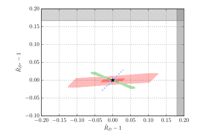
Maximal predictions for $\hat{R}_{D^{(*)}}-1$ from leptoquarks $V_{1},V_{3}$ and $S_{2}$ in flavor models are shown in Fig. 2. Not shown are predictions for $S_{1,3}$ , which are further suppressed as they either involve three powers of flavon VEVs or FN-suppression, as given by (41). The chirality-flipping contribution in $S_{1}$ is constrained by kaon decays, whereas, effectively, $S_{2}$ is not. The maximal predictions are obtained with single quarks being charged non-trivially under the non-abelian flavor symmetry.

Refer to caption — Figure 2: Maximal reach of leptoquarks $V_{1}$ (red), $V_{3}$ (blue) and $S_{2}$ (green) in $\hat{R}_{D^{*}}-1$ versus $\hat{R}_{D}-1$ in flavor models. Darker and lighter shaded areas correspond to FN-coefficients of $\pm 1$ and within $\pm(1/\sqrt{2};\sqrt{2})$ , respectively. The SM is denoted by the black star. Experimental $1\sigma$ regions (37) (grey) are shown only in the axes’ ranges displayed.

For each leptoquark, we show two ranges, one in which the $O(1)$ coefficients from the FN-mechanism have modulus 1 (darker shaded regions), and another one in which we allow for factors of $\sqrt{2}$ enhancement and suppression (lighter shaded regions). The latter results effectively in enlarging $YY^{*}$ by a factor 4, where a factor of 2 comes in directly and another one because the low energy constraints can be eased. For $V_{3}$ , shown in blue, we impose the kaon constraint on $c_{\nu}$ and require $c_{\ell}\lesssim 0.2$ . For $S_{2}$ (green) we employ the $\mu-e$ -conversion bounds on $\kappa c_{\nu}$ . For $V_{1}$ , shown in red, we employ the kaon bounds on $c_{\nu}$ and require $c_{\ell}\lesssim 0.2$ . For $V_{3}$ we also illustrate in dashing the region which would become accessible additionally if only the direct bound on $c_{\ell}c_{\nu}$ from $B\to K\nu\nu$ would be used. It shows that one is still $3\sigma$ away from the experimental $\hat{R}_{D^{*}}$ -band.

We learn that present data on $\hat{R}_{D}$ and $\hat{R}_{D^{*}}$ cannot be explained within $1.6\sigma$ and $3.1\sigma$ , respectively. Difficulties in explaining sizable BSM in $R_{D^{*}}$ have also been encountered within the context of Two-Higgs doublet models once conditions on the flavor structure are imposed [48].

The Belle II projection for the uncertainty on $R_{D}$ is $5.6\%\,(3.4\%)$ with $5\,{\rm ab}^{-1}\,(50\,{\rm ab}^{-1})$ and for $R_{D^{*}}$ is $3.2\%\,(2.1\%)$ for $5\,{\rm ab}^{-1}\,(50\,{\rm ab}^{-1})$ [49]. This suffices to probe all leptoquark models on the basis of branching ratio measurements even close to SM values.

The predictions for the $\tau$ -polarization are similar to the ones for $R_{D^{(*)}}$ with contributions from vector-like operators removed. $P_{\tau}(D^{*})$ can differ from the SM by at most a percent. Deviations from the SM in $P_{\tau}(D)$ can reach up to several percent. Present data on the $\tau$ -polarization, given in (37), are in agreement with the SM and are not sensitive to leptoquark flavor models yet.

IV.2 Leptoquark effects in $b\to s\ell\ell$

We analyze tree level leptoquark effects in $b\to s\ell\ell$ within the representations $S_{3},V_{1,2,3}$ and $\tilde{S}_{2}$ . We do not consider $S_{2}$ and $\tilde{S}_{1}$ because they induce only contributions onto operators $\bar{s}\gamma_{\mu}b\ell\gamma^{\mu}(1+\gamma_{5})\ell$ , whose impact on $B\to K^{(*)}\ell\ell$ branching ratios is very small. We focus on explaining the measurement of $R_{K}$ [50] by LHCb for dilepton masses squared between 1 and 6 $\mbox{GeV}^{2}$ [51]

\displaystyle R_{K}|_{[1,6]}=\frac{\mathcal{B}(B\to K\mu\mu)}{\mathcal{B}(B\to Kee)}=0.745\pm^{0.090}_{0.074}\pm 0.036\,.

(55)

A model-independent analysis points, at $1\sigma$ , to modifications to the vector-type operators $O_{9,10}^{(\prime)\ell}$ with couplings to $\ell=e,\mu$ as [21],

0.7\lesssim-\mathrm{Re}\left[C_{9}^{\text{NP}\mu}-C_{10}^{\text{NP}\mu}+C_{9}^{\prime\mu}-C_{10}^{\prime\mu}-\left(\mu\to e\right)\right]\lesssim 1.5\,,

(56)

where the operators are defined in Appendix C. Eq. (56) can be satisfied with $C_{9}^{\text{NP}\mu}=-C_{10}^{\text{NP}\mu}\sim Y^{b\mu}_{QL}\left(Y^{s\mu}_{QL}\right)^{*}$ or $Y^{s\mu}_{\bar{Q}L}\left(Y^{b\mu}_{\bar{Q}L}\right)^{*}$ with the leptoquarks $S_{3}$ , or $V_{1,3}$ , respectively, and

Y^{b\mu}_{QL}\left(Y^{s\mu}_{QL}\right)^{*}\text{ or }Y^{s\mu}_{\bar{Q}L}\left(Y^{b\mu}_{\bar{Q}L}\right)^{*}\simeq[0.001-0.002]\left(\frac{M}{\rm TeV}\right)^{2}\,.

(57)

Simple flavor patterns such as the $\mu$ -isolation one $L_{\mu}$ [7] can accommodate this

Y^{b\mu}_{QL}\left(Y^{s\mu}_{QL}\right)^{*}\text{ or }Y^{s\mu}_{\bar{Q}L}\left(Y^{b\mu}_{\bar{Q}L}\right)^{*}\sim c_{\ell}^{2}\lambda^{2}\,,

(58)

where $c_{\ell}\sim 0.2(M/\mbox{TeV})$ . Considering a natural value for the VEV this points to leptoquark masses below a few TeV. This is a stronger bound on $M$ than the one obtained in [21] by using $B_{s}-\bar{B}_{s}$ -mixing. $K\to\mu\mu$ decays, induced at order $c_{\ell}^{2}\lambda^{6}$ , and $\mu-e$ -conversion, after including mass basis corrections, arising at $O(c_{\ell}^{2}\delta\lambda^{8})$ , are both below their current limits.

With the second quark generation transforming non-trivially under $A_{4}$ the FN-suppression can be evaded. The corresponding patterns $\tilde{L}_{\mu}(QL,\bar{Q}L)$ are given in Eq. (31) and yield

Y^{b\mu}_{QL}\left(Y^{s\mu}_{QL}\right)^{*}\sim c_{\ell}c_{\nu}\kappa\,,\quad Y^{s\mu}_{\bar{Q}L}\left(Y^{b\mu}_{\bar{Q}L}\right)^{*}\sim c_{\ell}c_{\nu}\,,

(59)

for $S_{3}$ and $V_{1,3}$ , respectively. Eq. (57) can be accommodated with $c_{\ell}\sim 0.2(M/\mbox{TeV})$ and $c_{\nu}\kappa\sim 0.01(M/\mbox{TeV})$ ( $S_{3}$ ) and $c_{\nu}\sim 0.01(M/\mbox{TeV})$ ( $V_{1,3}$ ). The values of $\kappa c_{\nu}$ and $c_{\nu}$ are set to the upper limit allowed by kaon decays, induced at order $c_{\nu}^{2}\kappa^{2}\lambda^{2}$ and $c_{\nu}^{2}\lambda^{2}$ , respectively. As $c_{\ell}$ cannot be much larger a value of $R_{K}$ around (55) implies that the next round of LFV kaon and $\mu-e$ -experiments should see a signal.

BSM effects as in Eq. (56) can therefore be accommodated naturally with $S_{3},V_{3}$ with both $L_{\mu}$ and $\tilde{L}_{\mu}$ -patterns. Both leptoquark models induce also LFV in charm, however, due to the constraints from the kaon sector, effects in charm are very small. In $V_{1}$ both left- and right-handed couplings are present. The latter, $R_{\mu}(\bar{D}E)$ , moreover exhibits inverted flavor hierarchies, such that kaon decays are induced at order $\lambda$ , which seem to rule out $V_{1}$ with $\mu$ -isolation patterns. However, as discussed in Section II, it is viable to flip the sign of the charges $q(E)$ . In this case the hierarchies in $R_{\mu}(\bar{D}E)$ would increase. Contributions to kaon decays arise at $O(\lambda^{9})$ , which can be safely neglected. One-loop contributions to $\mu\to e\gamma$ arise in $V_{1}$ from $L_{\mu}\cdot R_{\mu}$ and $\tilde{L}_{\mu}\cdot R_{\mu}$ , which are enhanced by the top mass. Corresponding constraints from ${\cal{B}}(\mu\to e\gamma)<5.7\cdot 10^{-13}$ [46] read $c_{\ell}\delta\lambda^{4},c_{\nu}\lambda^{6}\lesssim 4\cdot 10^{-4}(M/\mbox{TeV})^{4}$ [3], which are always satisfied in our flavor models. Therefore, after adjusting lepton singlet charges, $V_{1}$ provides another viable scenario for explaining sizable $R_{K}$ .

One may employ the $\tau$ –isolation patterns of model $V_{3}$ discussed in the context of $R_{D^{(*)}}$ in Section IV.1.1 to predict $b\to s\mu\mu$ processes. The resulting effects are very small, further VEV-suppressed for $L_{\tau}(\bar{Q}L)$ as $\sim\delta^{2}c_{\ell}^{2}\lambda^{2}$ or constrained by $b\to s\nu\nu$ and low energy physics in $\tilde{L}_{\tau}(\bar{Q}L)$ as $\sim\delta c_{\ell}c_{\nu}+c_{\nu}^{2}\lambda^{2}$ . In either case, the effects are by orders of magnitude too small to match Eq. (56).

We consider now leptoquarks $\tilde{S}_{2}$ and $V_{2}$ , which induce right-handed currents $C_{9}^{\prime\mu}=-C_{10}^{\prime\mu}$ in $b\to s\ell\ell$ transitions. This is disfavored by global fits to data (excluding $R_{K}$ ) on $b\to s$ transitions, which suggests predominantly BSM in SM-type operators [52]. Let us nevertheless entertain this possibility as this line of research has not reached final conclusions yet. Right-handed currents would be signaled by $R_{K}\neq R_{K^{*}}$ [53], where $R_{K^{*}}$ denotes the ratio of branching fractions of $B\to K^{*}\mu\mu$ over the one into electrons. This part of our work is sensitive to the FN-charges of the down quark singlets, $q(D)$ . Let us therefore be here more general than the benchmark Eq. (2) and introduce $q_{i}\equiv q(D_{i})$ . Within the $L_{\mu}$ -pattern, where first (second) choice corresponds to $V_{2}$ ( $\tilde{S}_{2}$ ),

	$\displaystyle Y^{b\mu}_{DL}\left(Y^{s\mu}_{DL}\right)^{*}$	$\displaystyle\text{ or }Y^{s\mu}_{\bar{D}L}\left(Y^{b\mu}_{\bar{D}L}\right)^{*}\sim c_{\ell}^{2}\lambda^{q_{3}+q_{2}}\simeq[0.001-0.002]\penalty\ \mbox{or}\penalty\ [0.002-0.004]\left(\frac{M}{\rm TeV}\right)^{2}\,,$		(60)
	$\displaystyle Y^{s\mu}_{DL}\left(Y^{d\mu}_{DL}\right)^{*}$	$\displaystyle\text{ or }Y^{s\mu}_{\bar{D}L}\left(Y^{d\mu}_{\bar{D}L}\right)^{*}\sim c_{\ell}^{2}\lambda^{q_{2}+q_{1}}\lesssim 1.3\cdot 10^{-4}\penalty\ \mbox{or}\penalty\ 2.6\cdot 10^{-4}\left(\frac{M}{\rm TeV}\right)^{2}\,.$		(61)

Explaining $R_{K}$ (first row) while obeying limits from $K\to\mu\mu$ [34] (second row) strongly constrains the allowed values for the $q_{i}$ :

\displaystyle\lambda^{q_{1}-q_{3}}\lesssim 0.13\,,

(62)

which prefers $q_{1}\geq q_{3}+2$ . By perturbativity and lower limits on $M$ , $q_{2}+q_{3}=0,1,2,3$ . This is violated by the benchmark $q(D)=(3,2,2)$ , which requires $c_{\ell}\sim[0.8-1.2](M/\mbox{TeV})$ ( $V_{2}$ ) and $c_{\ell}\sim[1.2-1.7](M/\mbox{TeV})$ ( $\tilde{S}_{2}$ ). Both are not compatible with the flavor symmetry and mass bounds.

In supersymmetric or multi-Higgs extensions, a viable set reads $q(D)=(q_{3}+1,q_{3},q_{3})$ , where $q_{3}=0,1,2,3$ , all of which are in mild conflict with Eq. (62). When the charges of the quark doublets and up-type quarks are also changed, two viable solutions are $q(Q)=q(U)=(3,2,0)$ and $q(D)=(2,0,0)$ or $q(D)=(3,1,1)$ [26]. Smaller charges generically give smaller VEVs. Choosing $q(D)=(3,1,1)$ leads to

Y^{b\mu}_{DL}\left(Y^{s\mu}_{DL}\right)^{*}\text{ or }Y^{s\mu}_{\bar{D}L}\left(Y^{b\mu}_{\bar{D}L}\right)^{*}\sim c_{\ell}^{2}\lambda^{2}\,,

(63)

the same FN-hierarchy as for $S_{3},V_{1,3}$ obtained in Eq. (58). Therefore, $c_{\ell}\sim 0.2(M/\mbox{TeV})$ ( $V_{2}$ ) and $c_{\ell}\sim[0.2-0.3](M/\mbox{TeV})$ ( $\tilde{S}_{2}$ ), and, consequently, leptoquark masses should be within the few TeV-range. $\mu-e$ -conversion $\sim\delta c_{\ell}^{2}\lambda^{6}$ is below experimental limits. $\tilde{S}_{2}$ does not induce charm FCNCs at tree level.

Similar to the situation for $V_{1}$ discussed previously, in $V_{2}$ rapid kaon decays arise through $R_{\mu}(QE)$ . This can be avoided once the sign of $q(E)$ is flipped. In this case the constraint from $\mu\to e\gamma$ reads $c_{\ell}\delta\lambda^{3}\lesssim 10^{-4}(M/\mbox{TeV})^{4}$ [3], which is always satisfied for perturbative $\delta.$

We learn that improved bounds on kaon decays together with $b\to s\mu\mu$ data can strongly constrain or rule out BSM models with flavor patterns. If solutions with down quark singlets can be ruled out, this leads to testable predictions, the equality of LNU ratios $R_{K}$ and $R_{K^{*}}$ , as well as those of other $b\to s$ induced decay modes [53]. We checked that the impact of leptoquark models explaining $R_{K}$ at tree level on the observable ${\cal{B}}(B\to D^{(*)}\mu\nu)/{\cal{B}}(B\to D^{(*)}e\nu)$ [54] is at permille level. We further recall that $R_{K}$ -explaining leptoquarks can induce percent-level contributions to $b\to s\gamma$ and subsequently $b\to s\ell\ell$ spectra [21], which can be accessed at a future high luminosity facility (with 75 $\mbox{ab}^{-1}$ ) [55].

LFV in $b\to s\ell\ell^{\prime}$ transitions related to $R_{K}$ [56, 7, 57, 54] arises in the patterns studied in Eqs. (58) -(61). Relative to $b\to s\mu\mu$ the effects on the amplitudes read

	$\displaystyle b\to s\mu\mu$	$\displaystyle\penalty\ :\penalty\ b\to s\mu\,(e,\tau)\penalty\ :\penalty\ b\to se\tau\quad\mbox{as}\quad 1\penalty\ :\penalty\ \delta\penalty\ :\penalty\ \delta^{2}\quad\quad(L_{\mu})\,,$		(64)
	$\displaystyle b\to s\mu\mu$	$\displaystyle\penalty\ :\penalty\ b\to s\mu\,(e,\tau)\penalty\ :\penalty\ b\to se\tau\quad\mbox{as}\quad 1\penalty\ :\penalty\ 1\penalty\ :\penalty\ 1\quad\quad\penalty\ (\tilde{L}_{\mu})\,.$		(65)

The $\tilde{L}_{\mu}$ pattern predicts sizable LFV rates for leptonic and semileptonic $B_{(s)}$ -decays which can be searched for at future hadron colliders and $e^{+}e^{-}$ -machines, see [7] for details,

	$\displaystyle{\cal{B}}(B\to K\mu^{\pm}e^{\mp})$	$\displaystyle\sim 3\cdot 10^{-8}\left(\frac{1-R_{K}}{0.23}\right)^{2},\penalty\ {\cal{B}}(B\to K(e^{\pm},\mu^{\pm})\tau^{\mp})\sim 2\cdot 10^{-8}\left(\frac{1-R_{K}}{0.23}\right)^{2}\,,$		(66)
	$\displaystyle\frac{{\cal{B}}(B_{s}\to\mu^{+}e^{-})}{{\cal{B}}(B_{s}\to\mu^{+}\mu^{-})_{\rm SM}}$	$\displaystyle\sim 0.01\left(\frac{1-R_{K}}{0.23}\right)^{2}\,,\quad\frac{{\cal{B}}(B_{s}\to\tau^{+}(e^{-},\mu^{-}))}{{\cal{B}}(B_{s}\to\mu^{+}\mu^{-})_{\rm SM}}\sim 4\left(\frac{1-R_{K}}{0.23}\right)^{2}\,.$		(67)

IV.3 Leptoquark effects in rare charm and kaon decays and $\mu-e$ conversion

We investigate the implications of the flavor patterns studied in the previous sections for rare charm decays, $K$ decays and $\mu-e$ -conversion.

Using [8] we find the following maximal upper limits, where the corresponding scenario and pattern is indicated in parentheses: $\mathcal{B}(D\to\pi\nu\nu)\lesssim$3\text{⋅}{10}^{-10}$$ ( $(S_{3},V_{3})$ , $L_{\mu}$ ), $\mathcal{B}(D\to\pi e\mu)\lesssim$3\text{⋅}{10}^{-13}$$ ( $V_{3}$ , $L_{\mu}$ ), $\mathcal{B}(D\to e\mu)\lesssim$5\text{⋅}{10}^{-15}$$ ( $V_{3}$ , $\tilde{L}_{\mu}$ ) and $\mathcal{B}(D\to e\tau)\lesssim$7\text{⋅}{10}^{-17}$$ ( $S_{2}$ , $\tilde{L}_{\tau}$ ). $\mathcal{B}(D\to\mu\mu)$ and $\mathcal{B}(D\to\pi\mu\mu)$ are SM-like. Note, $\mathcal{B}^{\text{SM}}(D\to\mu\mu)\sim 10^{-13}$ and $\mathcal{B}^{\text{SM}}(D\to\pi\mu\mu)\sim 10^{-12}$ (non-resonant). These BSM effects in charm are below present experimental limits by many orders of magnitude. The reason is the presence of the kaon constraints, which are unavoidable once doublet quarks are involved. These are, however, not the largest possible signatures in charm accociated with leptoquarks in flavor models, but the largest associated with models addressing $R_{D^{(*)}}$ and $R_{K}$ .

In scenario $\tilde{V}_{1}$ with the skewed pattern $R_{\mu e}(\bar{U}E)$ , which could have a large impact on rare charm decays, the FN-suppression of the $(1,2)$ element is not strong enough to effectively evade the $\mu-e$ conversion constraint, while, at the same time, keep the diagonal ones sizable. Similarly, effects in rare charm processes from $S_{1}$ with $R_{\tau}(UE)$ are $Y^{c\ell}_{UE}Y_{UE}^{u\ell*}\sim\delta^{(\prime)}\lambda^{10}$ , and negligible compared to the foreseeable experimental sensitivity. With the skewed pattern $R_{e\tau}$ and leptoquark $\tilde{V}_{1}$ $\mu-e$ conversion constraints can be evaded and $c\to ue\tau$ transitions can be induced at order $\kappa\kappa^{\prime}\lambda^{2}\lesssim$1\text{⋅}{10}^{-3}$$ . This leads to $\mathcal{B}(D\to e\tau)\lesssim$1\text{⋅}{10}^{-13}$$ .

The leptoquarks $S_{3}$ and $V_{3}$ are constrained by LFV kaon decays, therefore large contributions near the experimental bound $\mathcal{B}(K_{L}\to e\mu)<$4.7\text{⋅}{10}^{-12}$$ [58] are expected. The model ( $S_{2}$ , $(\tilde{L}_{\tau},R_{\tau})$ ) is bound by $\mu-e$ conversion and contributes less to rare kaon decays. We find $\mathcal{B}(K_{L}\to e\mu)\lesssim$4\text{⋅}{10}^{-19}$$ .

Future $\mu-e$ -conversion experiments such as COMET [59] and Mu2e [60] with sensitivity below $10^{-16}$ , that is 2-3 orders of magnitude better than the existing bounds, are sensitive to the leptoquarks $S_{3}$ and $V_{3}$ with $\tilde{L}_{\mu}$ discussed here. We find $\frac{\sigma(\mu^{-}\text{Au}\to e^{-}\text{Au})}{\sigma(\mu^{-}\text{Au}\to\text{capture})}\lesssim$2\text{⋅}{10}^{-13}$($5\text{⋅}{10}^{-14}$)$ for $V_{3}$ (for $S_{3}$ ).

V Conclusions

We obtain patterns for leptoquark couplings to SM fermions based on flavor symmetries. In addition to those for lepton doublets [7], we find lepton isolation patterns for charged lepton singlets. These are particularly relevant for contributions to $R_{D^{(*)}}$ involving both chiralities. We argue on general terms that chirality-flipping contributions are generically larger than the ones based on SM-like operators involving doublet lepton couplings.

The flavor symmetry puts strong constraints on the leptoquark reach in flavor observables. We find that it is not possible to explain the present data on $R_{D}$ and $R_{D}^{*}$ from tree level leptoquark exchange. The reason is that these BSM effects of few $\times 0.1$ are too large given lower mass bounds on the leptoquarks, perturbativity of the flavor symmetry breaking and flavor constraints, importantly, $b\to s\nu\bar{\nu}$ , rare kaon decays and $\mu-e$ -conversion. We give predictions for $R_{D}$ , $R_{D^{*}}$ and the $\tau$ -polarization, which are summarized in Section IV.1.4. At least the maximal leptoquark models, shown in Fig. 2, can be tested at Belle II with $50{\rm ab}^{-1}$ [61].

On the other hand, $R_{K}$ together with the preferred global fit in $b\to s$ observables can be explained naturally using muon isolation patterns and $S_{3},V_{3}$ . If one abandons the constraints from the global fit, which prefers predominantly $V-A$ -structure, model $\tilde{S}_{2}$ accommodates as well a few $\times 0.1$ BSM effect in semileptonic $b\to s\mu\mu$ processes. $\tilde{S}_{2}$ also predicts $R_{K}\neq R_{K^{*}}$ .

In our analysis we require the non-abelian flavon VEVs to remain perturbative, or we constrain them experimentally. As we do not rely on model-dependent values our findings are more general than the explicit $U(1)_{\text{FN}}\times A_{4}\times Z_{3}$ model under consideration.

Since the current LNU hints in $R_{D}$ and in particular $R_{D^{*}}$ are too large to be accommodated with leptoquark flavor patterns, there are also no joint explanations with $R_{K}$ . If both anomalies persist at the current level, additional BSM-physics would be required. To have in both $R_{K}$ and $R_{D^{(*)}}$ LNU effects maximized from leptoquark flavor patterns requires two types of leptoquarks, with masses of at most at the level of several TeV. LFV signatures can be searched for with kaon decays and $\mu-e$ conversion.

Acknowledgements.

We are happy to thank Stefan de Boer, Nejc Kosnik, Ivo de Medeiros Varzielas, Ivan Nisandzic and Erik Schumacher for useful discussions. GH is grateful to the Aspen Center for Physics where this project was finalized for its hospitality and stimulating environment. The Aspen Center for Physics is supported by National Science Foundation grant PHY-1066293. This work is supported by the Bundesministerium für Bildung und Forschung (BMBF).

Appendix A Leptoquark couplings to SM fermions

$\subset\mathcal{L}_{\text{LQ}}$	$(SU(3)_{C},SU(2)_{L},Y)$	effective vertices
$\left(Y_{QL}\bar{Q}_{\text{L}}^{c}i\sigma_{2}L_{\text{L}}+Y_{UE}\bar{u}_{\text{R}}^{c}e_{\text{R}}\right)S_{1}^{\dagger}$	(3,1,-1/3)	$\frac{Y_{QL}^{ij}\left(Y_{QL}^{mn}\right)^{*}}{2M^{2}}(\bar{u}_{\text{L}m}\gamma_{\mu}u_{\text{L}i})(\bar{\ell}_{\text{L}n}\gamma^{\mu}\ell_{\text{L}j})$
		$-\frac{Y_{QL}^{ij}\left(Y_{QL}^{mn}\right)^{*}}{2M^{2}}(\bar{u}_{\text{L}m}\gamma_{\mu}d_{\text{L}i})(\bar{\ell}_{\text{L}n}\gamma^{\mu}\nu_{\text{L}j})$
		$\frac{Y_{QL}^{ij}\left(Y_{QL}^{mn}\right)^{*}}{2M^{2}}(\bar{d}_{\text{L}m}\gamma_{\mu}d_{\text{L}i})(\bar{\nu}_{\text{L}n}\gamma^{\mu}\nu_{\text{L}j})$
		$\frac{Y_{UE}^{ij}\left(Y_{UE}^{mn}\right)^{*}}{2M^{2}}(\bar{u}_{\text{R}m}\gamma_{\mu}u_{\text{R}i})(\bar{\ell}_{\text{R}n}\gamma^{\mu}\ell_{\text{R}j})$
		$-\frac{Y_{QL}^{ij}\left(Y_{UE}^{mn}\right)^{*}}{2M^{2}}(\bar{u}_{\text{R}m}u_{\text{L}i})(\bar{\ell}_{\text{R}n}\ell_{\text{L}j})$
		$\frac{Y_{QL}^{ij}\left(Y_{UE}^{mn}\right)^{*}}{8M^{2}}(\bar{u}_{\text{R}m}\sigma_{\mu\nu}u_{\text{L}i})(\bar{\ell}_{\text{R}n}\sigma^{\mu\nu}\ell_{\text{L}j})$
		$\frac{Y_{QL}^{ij}\left(Y_{UE}^{mn}\right)^{*}}{2M^{2}}(\bar{u}_{\text{R}m}d_{\text{L}i})(\bar{\ell}_{\text{R}n}\nu_{\text{L}j})$
		$-\frac{Y_{QL}^{ij}\left(Y_{UE}^{mn}\right)^{*}}{8M^{2}}(\bar{u}_{\text{R}m}\sigma_{\mu\nu}d_{\text{L}i})(\bar{\ell}_{\text{R}n}\sigma^{\mu\nu}\nu_{\text{L}j})$
$Y_{DE}\bar{d}_{\text{R}}^{c}e_{\text{R}}\tilde{S_{1}}^{\dagger}$	(3,1,-4/3)	$\frac{Y_{DE}^{ij}\left(Y_{DE}^{mn}\right)^{*}}{2M^{2}}(\bar{d}_{\text{R}m}\gamma_{\mu}d_{\text{R}i})(\bar{e}_{\text{R}n}\gamma^{\mu}e_{\text{R}j})$
$\left(Y_{\bar{U}L}\bar{u}_{\text{R}}L_{\text{L}}+Y_{\bar{Q}E}\bar{Q}_{\text{L}}i\sigma_{2}e_{\text{R}}\right)S_{2}^{\dagger}$	(3,2,-7/6)	$-\frac{Y_{\bar{U}L}^{ij}\left(Y_{\bar{U}L}^{mn}\right)^{*}}{2M^{2}}(\bar{u}_{\text{R}i}\gamma_{\mu}u_{\text{R}m})(\bar{\nu}_{\text{L}n}\gamma^{\mu}\nu_{\text{L}j})$
		$-\frac{Y_{\bar{U}L}^{ij}\left(Y_{\bar{U}L}^{mn}\right)^{*}}{2M^{2}}(\bar{u}_{\text{R}i}\gamma_{\mu}u_{\text{R}m})(\bar{\ell}_{\text{L}n}\gamma^{\mu}\ell_{\text{L}j})$
		$-\frac{Y_{\bar{Q}E}^{ij}\left(Y_{\bar{Q}E}^{mn}\right)^{*}}{2M^{2}}(\bar{u}_{\text{L}i}\gamma_{\mu}u_{\text{L}m})(\bar{\ell}_{\text{R}n}\gamma^{\mu}\ell_{\text{R}j})$
		$-\frac{Y_{\bar{Q}E}^{ij}\left(Y_{\bar{Q}E}^{mn}\right)^{*}}{2M^{2}}(\bar{d}_{\text{L}i}\gamma_{\mu}d_{\text{L}m})(\bar{\ell}_{\text{R}n}\gamma^{\mu}\ell_{\text{R}j})$
		$\frac{Y_{\bar{U}L}^{ij}\left(Y_{\bar{Q}E}^{mn}\right)^{*}}{2M^{2}}(\bar{u}_{\text{R}i}d_{\text{L}m})(\bar{\ell}_{\text{R}n}\nu_{\text{L}j})$
		$\frac{Y_{\bar{U}L}^{ij}\left(Y_{\bar{Q}E}^{mn}\right)^{*}}{8M^{2}}(\bar{u}_{\text{R}i}\sigma_{\mu\nu}d_{\text{L}m})(\bar{\ell}_{\text{R}n}\sigma^{\mu\nu}\nu_{\text{L}j})$
		$-\frac{Y_{\bar{U}L}^{ij}\left(Y_{\bar{Q}E}^{mn}\right)^{*}}{2M^{2}}(\bar{u}_{\text{R}i}u_{\text{L}m})(\bar{\ell}_{\text{R}n}\ell_{\text{L}j})$
		$-\frac{Y_{\bar{U}L}^{ij}\left(Y_{\bar{Q}E}^{mn}\right)^{*}}{8M^{2}}(\bar{u}_{\text{R}i}\sigma_{\mu\nu}u_{\text{L}m})(\bar{\ell}_{\text{R}n}\sigma^{\mu\nu}\ell_{\text{L}j})$
$Y_{\bar{D}L}\bar{d}_{\text{R}}L_{\text{L}}\tilde{S}_{2}^{\dagger}$	(3,2,1/6)	$-\frac{Y_{\bar{D}L}^{ij}\left(Y_{\bar{D}L}^{mn}\right)^{*}}{2M^{2}}(\bar{d}_{\text{R}i}\gamma_{\mu}d_{\text{R}m})(\bar{\nu}_{\text{L}n}\gamma^{\mu}\nu_{\text{L}j})$
		$-\frac{Y_{\bar{D}L}^{ij}\left(Y_{\bar{D}L}^{mn}\right)^{*}}{2M^{2}}(\bar{d}_{\text{R}i}\gamma_{\mu}d_{\text{R}m})(\bar{\ell}_{\text{L}n}\gamma^{\mu}\ell_{\text{L}j})$
$Y_{QL}\bar{Q}_{\text{L}}^{c}i\sigma_{2}\vec{\sigma}L_{\text{L}}\vec{S}_{3}^{\dagger}$	(3,3,-1/3)	$\frac{Y_{QL}^{ij}\left(Y_{QL}^{mn}\right)^{*}}{M^{2}}(\bar{u}_{\text{L}m}\gamma_{\mu}u_{\text{L}i})(\bar{\nu}_{\text{L}n}\gamma^{\mu}\nu_{\text{L}j})$
		$\frac{Y_{QL}^{ij}\left(Y_{QL}^{mn}\right)^{*}}{M^{2}}(\bar{d}_{\text{L}m}\gamma_{\mu}d_{\text{L}i})(\bar{\ell}_{\text{L}n}\gamma^{\mu}\ell_{\text{L}j})$
		$\frac{Y_{QL}^{ij}\left(Y_{QL}^{mn}\right)^{*}}{2M^{2}}(\bar{u}_{\text{L}m}\gamma_{\mu}u_{\text{L}i})(\bar{\ell}_{\text{L}n}\gamma^{\mu}\ell_{\text{L}j})$
		$\frac{Y_{QL}^{ij}\left(Y_{QL}^{mn}\right)^{*}}{2M^{2}}(\bar{u}_{\text{L}m}\gamma_{\mu}d_{\text{L}i})(\bar{\ell}_{\text{L}n}\gamma^{\mu}\nu_{\text{L}j})$
		$\frac{Y_{QL}^{ij}\left(Y_{QL}^{mn}\right)^{*}}{2M^{2}}(\bar{d}_{\text{L}m}\gamma_{\mu}d_{\text{L}i})(\bar{\nu}_{\text{L}n}\gamma^{\mu}\nu_{\text{L}j})$

Table 5: Scalar leptoquark models and their respective effective vertices at tree level.

Q

denotes the

SU(2)_{L}

doublet

(u_{L}\ d_{L})

, with

u=u,c,t

;

d=d,s,b

;

\ell=e,\mu,\tau

and

\nu=\nu_{e},\nu_{\mu},\nu_{\tau}

. Small roman indices are generation indices and are supressed in the first column.

Y=Q_{e}-I_{3}

is the hypercharge,

Q_{e}

the electric charge and

I_{3}

the third component of the weak isospin.

$\subset\mathcal{L}_{\text{LQ}}$	$(SU(3)_{C},SU(2)_{L},Y)$	effective vertices
$\left(Y_{\bar{Q}L}\bar{Q}_{\text{L}}\gamma_{\mu}L_{\text{L}}+Y_{\bar{D}E}\bar{d}_{\text{R}}\gamma_{\mu}e_{\text{R}}\right)V_{1}^{\mu\dagger}$	(3,1,-1/6)	$-\frac{Y_{\bar{Q}L}^{ij}\left(Y_{\bar{Q}L}^{mn}\right)^{*}}{M^{2}}(\bar{u}_{\text{L}i}\gamma_{\mu}u_{\text{L}m})(\bar{\nu}_{\text{L}n}\gamma^{\mu}\nu_{\text{L}j})$
		$-\frac{Y_{\bar{Q}L}^{ij}\left(Y_{\bar{Q}L}^{mn}\right)^{*}}{M^{2}}(\bar{u}_{\text{L}i}\gamma_{\mu}d_{\text{L}m})(\bar{\ell}_{\text{L}n}\gamma^{\mu}\nu_{\text{L}j})$
		$-\frac{Y_{\bar{Q}L}^{ij}\left(Y_{\bar{Q}L}^{mn}\right)^{*}}{M^{2}}(\bar{d}_{\text{L}i}\gamma_{\mu}d_{\text{L}m})(\bar{\ell}_{\text{L}n}\gamma^{\mu}\ell_{\text{L}j})$
		$-\frac{Y_{\bar{D}E}^{ij}\left(Y_{\bar{D}E}^{mn}\right)^{*}}{M^{2}}(\bar{d}_{\text{R}i}\gamma_{\mu}d_{\text{R}m})(\bar{\ell}_{\text{R}n}\gamma^{\mu}\ell_{\text{R}j})$
		$\frac{2Y_{\bar{Q}L}^{ij}\left(Y_{\bar{D}E}^{mn}\right)^{*}}{M^{2}}(\bar{u}_{\text{L}i}d_{\text{R}m})(\bar{\ell}_{\text{R}n}\nu_{\text{L}j})$
		$\frac{2Y_{\bar{Q}L}^{ij}\left(Y_{\bar{D}E}^{mn}\right)^{*}}{M^{2}}(\bar{d}_{\text{L}i}d_{\text{R}m})(\bar{\ell}_{\text{R}n}\ell_{\text{L}j})$
$Y_{\bar{U}E}\bar{u}_{\text{R}}\gamma_{\mu}e_{\text{R}}\tilde{V}_{1}^{\mu\dagger}$	(3,1,5/3)	$-\frac{Y_{\bar{U}E}^{ij}\left(Y_{\bar{U}E}^{mn}\right)^{*}}{M^{2}}(\bar{u}_{\text{R}i}\gamma_{\mu}u_{\text{R}m})(\bar{\ell}_{\text{R}n}\gamma^{\mu}\ell_{\text{R}j})$
$\left(Y_{DL}\bar{d}_{\text{R}}^{c}\gamma_{\mu}L_{\text{L}}+Y_{QE}\bar{Q}_{\text{L}}^{c}\gamma_{\mu}e_{\text{R}}\right)i\sigma_{2}V_{2}^{\mu\dagger}$	(3,2,-5/6)	$\frac{Y_{DL}^{ij}\left(Y_{DL}^{mn}\right)^{*}}{M^{2}}(\bar{d}_{\text{R}m}\gamma_{\mu}d_{\text{R}i})(\bar{\nu}_{\text{L}n}\gamma^{\mu}\nu_{\text{L}j})$
		$\frac{Y_{DL}^{ij}\left(Y_{DL}^{mn}\right)^{*}}{M^{2}}(\bar{d}_{\text{R}m}\gamma_{\mu}d_{\text{R}i})(\bar{\ell}_{\text{L}n}\gamma^{\mu}\ell_{\text{L}j})$
		$\frac{Y_{QE}^{ij}\left(Y_{QE}^{mn}\right)^{*}}{M^{2}}(\bar{u}_{\text{L}m}\gamma_{\mu}u_{\text{L}i})(\bar{\ell}_{\text{R}n}\gamma^{\mu}\ell_{\text{R}j})$
		$\frac{Y_{QE}^{ij}\left(Y_{QE}^{mn}\right)^{*}}{M^{2}}(\bar{d}_{\text{L}m}\gamma_{\mu}d_{\text{L}i})(\bar{\ell}_{\text{R}n}\gamma^{\mu}\ell_{\text{R}j})$
		$\frac{2Y_{DL}^{ij}\left(Y_{QE}^{mn}\right)^{*}}{M^{2}}(\bar{u}_{\text{L}m}d_{\text{R}i})(\bar{\ell}_{\text{R}n}\nu_{\text{L}j})$
		$\frac{2Y_{DL}^{ij}\left(Y_{QE}^{mn}\right)^{*}}{M^{2}}(\bar{d}_{\text{L}m}d_{\text{R}i})(\bar{\ell}_{\text{R}n}\ell_{\text{L}j})$
$Y_{UL}\bar{u}_{\text{R}}^{c}\gamma_{\mu}L_{L}\tilde{V}_{2}^{\mu\dagger}$	(3,2,1/6)	$\frac{Y_{UL}^{ij}\left(Y_{UL}^{mn}\right)^{*}}{M^{2}}(\bar{u}_{\text{R}m}\gamma_{\mu}u_{\text{R}i})(\bar{\nu}_{\text{L}n}\gamma^{\mu}\nu_{\text{L}j})$
		$\frac{Y_{UL}^{ij}\left(Y_{UL}^{mn}\right)^{*}}{M^{2}}(\bar{u}_{\text{R}m}\gamma_{\mu}u_{\text{R}i})(\bar{\ell}_{\text{L}n}\gamma^{\mu}\ell_{\text{L}j})$
$Y_{\bar{Q}L}\bar{Q}_{\text{L}}\gamma_{\mu}\vec{\sigma}L_{\text{L}}\vec{V}_{3}^{\mu\dagger}$	(3,3,-2/3)	$-\frac{2Y_{\bar{Q}L}^{ij}\left(Y_{\bar{Q}L}^{mn}\right)^{*}}{M^{2}}(\bar{u}_{\text{L}i}\gamma_{\mu}u_{\text{L}m})(\bar{\ell}_{\text{L}n}\gamma^{\mu}\ell_{\text{L}j})$
		$-\frac{2Y_{\bar{Q}L}^{ij}\left(Y_{\bar{Q}L}^{mn}\right)^{*}}{M^{2}}(\bar{d}_{\text{L}i}\gamma_{\mu}d_{\text{L}m})(\bar{\nu}_{\text{L}n}\gamma^{\mu}\nu_{\text{L}j})$
		$-\frac{Y_{\bar{Q}L}^{ij}\left(Y_{\bar{Q}L}^{mn}\right)^{*}}{M^{2}}(\bar{u}_{\text{L}i}\gamma_{\mu}u_{\text{L}m})(\bar{\nu}_{\text{L}n}\gamma^{\mu}\nu_{\text{L}j})$
		$\frac{Y_{\bar{Q}L}^{ij}\left(Y_{\bar{Q}L}^{mn}\right)^{*}}{M^{2}}(\bar{u}_{\text{L}i}\gamma_{\mu}d_{\text{L}m})(\bar{\ell}_{\text{L}n}\gamma^{\mu}\nu_{\text{L}j})$
		$-\frac{Y_{\bar{Q}L}^{ij}\left(Y_{\bar{Q}L}^{mn}\right)^{*}}{M^{2}}(\bar{d}_{\text{L}i}\gamma_{\mu}d_{\text{L}m})(\bar{\ell}_{\text{L}n}\gamma^{\mu}\ell_{\text{L}j})$

Table 6: Same as Table 5 but for vector leptoquark models.

Appendix B $b\to c\ell\nu$

The effective Hamiltonian for $b\to c\ell\nu$ transitions can be written as

\mathcal{H}_{\text{eff}}^{b\to c\ell\nu}=\frac{4G_{\text{F}}}{\sqrt{2}}V_{cb}\left(\delta_{\ell\nu}\mathcal{O}_{V_{1}}^{\ell\nu}+\sum_{i}C_{i}^{\ell\nu}\mathcal{O}_{i}^{\ell\nu}\right)\,,

(68)

where

$\displaystyle\mathcal{O}_{V_{1(2)}}^{\ell\nu}$	$\displaystyle=\left[\bar{c}_{\text{L(R)}}\gamma^{\mu}b_{\text{L(R)}}\right]\left[\bar{\ell}_{\text{L}}\gamma_{\mu}\nu_{\text{L}}\right]\,,$	(69)
$\displaystyle\mathcal{O}_{S_{1(2)}}^{\ell\nu}$	$\displaystyle=\left[\bar{c}_{\text{L(R)}}b_{\text{R(L)}}\right]\left[\bar{\ell}_{\text{R}}\nu_{\text{L}}\right]\,,$
$\displaystyle\mathcal{O}_{T}^{\ell\nu}$	$\displaystyle=\left[\bar{c}_{\text{R}}\sigma^{\mu\nu}b_{\text{L}\vphantom{(}}\right]\left[\bar{\ell}_{\text{R}}\sigma_{\mu\nu}\nu_{\text{L}}\right]\,.$

In the SM, all Wilson coefficients $C_{i}^{\ell\nu}$ vanish. Tree level contributions from leptoquarks are given in Table 11, where $\tilde{C}\equiv\frac{4G_{\text{F}}}{\sqrt{2}}V_{cb}M^{2}C$ is used for brevity ³³ 3 The chirality-flipping contribution given in Table 3 of [62] for $S=0$ misses an overall sign. We thank Nejc Kosnik for clarification.. Contributions to $\mathcal{O}_{V_{2}}^{\ell\nu}$ are not induced at leading order.

The energy scale dependence of the Wilson coefficients is governed by renormalization group equations. At leading logarithmic order holds [63, 64]

	$\displaystyle C_{S}(\mu_{b})$	$\displaystyle=\left[\frac{\alpha_{s}(m_{t})}{\alpha_{s}(\mu_{b})}\right]^{\frac{\gamma_{S}}{2\beta_{0}^{(5)}}}\left[\frac{\alpha_{s}(M)}{\alpha_{s}(m_{t})}\right]^{\frac{\gamma_{S}}{2\beta_{0}^{(6)}}}C_{S}(M)\,,$	$\displaystyle C_{S}(\mu_{c})$	$\displaystyle=\left[\frac{\alpha_{s}(\mu_{b})}{\alpha_{s}(\mu_{c})}\right]^{\frac{\gamma_{S}}{2\beta_{0}^{(4)}}}C_{S}(\mu_{b})\,,$		(70)
	$\displaystyle C_{T}(\mu_{b})$	$\displaystyle=\left[\frac{\alpha_{s}(m_{t})}{\alpha_{s}(\mu_{b})}\right]^{\frac{\gamma_{T}}{2\beta_{0}^{(5)}}}\left[\frac{\alpha_{s}(M)}{\alpha_{s}(m_{t})}\right]^{\frac{\gamma_{T}}{2\beta_{0}^{(6)}}}C_{T}(M)\,,$	$\displaystyle C_{T}(\mu_{c})$	$\displaystyle=\left[\frac{\alpha_{s}(\mu_{b})}{\alpha_{s}(\mu_{c})}\right]^{\frac{\gamma_{T}}{2\beta_{0}^{(4)}}}C_{T}(\mu_{b})$		(71)

with

\displaystyle\gamma_{S}

\displaystyle=-8\,,

\displaystyle\gamma_{T}

\displaystyle=\frac{8}{3}\,,\quad

\displaystyle\beta_{0}^{(n_{f})}=11-\frac{2n_{f}}{3}\,.

(72)

We use the CRunDec package [65] to evaluate $\alpha_{s}$ . Assuming $M\sim 1\text{TeV}$ we find a modification of the Fierz relations between scalar and tensor operators, $C_{S}(M)=\mp 4C_{T}(M)$ , at the $b$ - and $c$ -quark mass scale, $\mu_{b}$ and $\mu_{c}$ , respectively,

	$\displaystyle C_{S}(\mu_{b})$	$\displaystyle=\mp\begin{cases}7.8C_{T}(\mu_{b})\ M=$1\text{\,}\mathrm{T}\mathrm{e}\mathrm{V}$\\ 8.2C_{T}(\mu_{b})\ M=$2\text{\,}\mathrm{T}\mathrm{e}\mathrm{V}$\\ 8.4C_{T}(\mu_{b})\ M=$3\text{\,}\mathrm{T}\mathrm{e}\mathrm{V}$\end{cases},$		(73)
	$\displaystyle C_{S}(\mu_{c})$	$\displaystyle=\mp\begin{cases}11.0C_{T}(\mu_{c})\ M=$1\text{\,}\mathrm{T}\mathrm{e}\mathrm{V}$\\ 11.6C_{T}(\mu_{c})\ M=$2\text{\,}\mathrm{T}\mathrm{e}\mathrm{V}$\\ 12.0C_{T}(\mu_{c})\ M=$3\text{\,}\mathrm{T}\mathrm{e}\mathrm{V}$\end{cases}\,,$		(74)

where the minus sign (plus sign) refers to scenario $S_{1}$ ( $S_{2}$ ). The overall running of $C_{S}$ and $C_{T}$ is negligible compared to the unknown $\mathcal{O}(1)$ coefficients of the flavor patterns and will not be considered further.

The branching fractions of $B\to D^{(*)}\ell\nu$ decays can be written as

\begin{split}\mathcal{B}(B\to D\ell\nu)=&\sum\limits_{\nu}\mathcal{B}^{\text{SM}}(B\to D\ell\nu)|\delta_{\ell\nu}+C_{V_{1}}^{\ell\nu}+C_{V_{2}}^{\ell\nu}|^{2}+A_{S}|C_{S_{1}}^{\ell\nu}+C_{S_{2}}^{\ell\nu}|^{2}\\ &+A_{T}|C_{T}^{\ell\nu}|^{2}+A_{VS}\text{Re}\left[(\delta_{\ell\nu}+C_{V_{1}}^{\ell\nu}+C_{V_{2}}^{\ell\nu})(C_{S_{1}}^{\ell\nu}+C_{S_{2}}^{\ell\nu})^{*}\right]\\ &+A_{VT}\text{Re}\left[(\delta_{\ell\nu}+C_{V_{1}}^{\ell\nu}+C_{V_{2}}^{\ell\nu})C_{T}^{\ell\nu*}\right]\,,\end{split}

(75)

\begin{split}\mathcal{B}(B\to D^{*}\ell\nu)=&\sum\limits_{\nu}\mathcal{B}^{\text{SM}}(B\to D^{*}\ell\nu)\left[|\delta_{\ell\nu}+C_{V_{1}}^{\ell\nu}|^{2}+|C_{V_{2}}^{\ell\nu}|^{2}\right]\\ &+B_{V_{1}V_{2}}\text{Re}\left[(\delta_{\ell\nu}+C_{V_{1}}^{\ell\nu})C_{V_{2}}^{\ell\nu*}\right]+B_{S}|C_{S_{1}}^{\ell\nu}-C_{S_{2}}^{\ell\nu}|^{2}+B_{T}|C_{T}^{\ell\nu}|^{2}\\ &+B_{VS}\text{Re}\left[(\delta_{\ell\nu}+C_{V_{1}}^{\ell\nu}-C_{V_{2}}^{\ell\nu})(C_{S_{1}}^{\ell\nu}-C_{S_{2}}^{\ell\nu})^{*}\right]\\ &+B_{V_{1}T}\text{Re}\left[(\delta_{\ell\nu}+C_{V_{1}}^{\ell\nu})C_{T}^{\ell\nu*}\right]+B_{V_{2}T}\text{Re}\left[C_{V_{2}}^{\ell\nu}C_{T}^{\ell\nu*}\right]\,,\end{split}

(76)

where the coefficients $A_{i}$ and $B_{i}$ generally depend on the lepton and its polarization. Corresponding indices are suppressed in Eqs. (75), (76) to avoid clutter. The coefficients can be expressed in terms of hadronic matrix elements provided in Ref. [10]. Using lattice data from [35] for the $B\to D$ form factors and the HQET form factors from [10] for $B\to D^{*}$ , we find the numerical values given in Tables 7 and 8 by integrating over the whole $q^{2}$ -range, summing over the lepton-polarization and normalizing to the SM branching ratios. For the latter we obtain $\mathcal{B}^{\text{SM}}(B^{0}\to D^{+}\tau\nu)=$6.66\pm\pm 0.67\text{⋅}{10}^{-3}$$ , $\mathcal{B}^{\text{SM}}(B^{0}\to D^{+}(e,\mu)\nu)=$2.23\pm\pm 0.24\text{⋅}{10}^{-2}$$ and $\mathcal{B}^{\text{SM}}(B^{0}\to D^{+*}\tau\nu)=$1.35\pm\pm 0.10\text{⋅}{10}^{-2}$$ , $\mathcal{B}^{\text{SM}}(B^{0}\to D^{+*}(e,\mu)\nu)=$5.34\pm\pm 0.40\text{⋅}{10}^{-2}$$ . Here we use the lifetime $\tau_{B^{0}}=$1.520\pm\pm 0.004\text{⋅}{10}^{-12}\text{\,}\mathrm{s}$$ of the $B^{0}$ meson [46]. In order to estimate the uncertainties, we draw ${10}^{5}$ random samples of the form factor parameters provided in the respective references and calculate the coefficients $A_{i}$ and $B_{i}$ for each sample. The mean and standard deviation of the resulting distributions are then considered as the central value and uncertainty. We assume that the form factor parameters are normally distributed and incorperate all correlations provided by [35, 10].

Additionally, we provide the coefficients for given $\tau$ -polarizations in Tables 9 and 10, where we normalize to the difference $\mathcal{B}^{\text{SM}}_{k=+}-\mathcal{B}^{\text{SM}}_{k=-}$ of the SM values of the polarized branching fractions. For the latter we obtain $\mathcal{B}^{\text{SM}}_{k=+}(B^{0}\to D^{+}\tau\nu)=$4.43\pm\pm 0.47\text{⋅}{10}^{-3}$$ , $\mathcal{B}^{\text{SM}}_{k=-}(B^{0}\to D^{+}\tau\nu)=$2.22\pm\pm 0.22\text{⋅}{10}^{-3}$$ , and $\mathcal{B}^{\text{SM}}_{k=+}(B^{0}\to D^{+*}\tau\nu)=$3.40\pm\pm 0.27\text{⋅}{10}^{-3}$$ , $\mathcal{B}^{\text{SM}}_{k=-}(B^{0}\to D^{+*}\tau\nu)=$1.01\pm\pm 0.07\text{⋅}{10}^{-2}$$ . Scalar operators do not contribute to the case where $k=-$ .

$\ \ell\$	$\hat{A}_{S}^{\ell}$	$\hat{A}_{T}^{\ell}$	$\hat{A}_{VS}^{\ell}$	$\hat{A}_{VT}^{\ell}$
$e$	$1.45$ 0.16	$0.38$ 0.20	$0.00$ 0.00	$0.00$ 0.00
$\mu$	$1.45$ 0.16	$0.36$ 0.17	$0.17$ 0.02	$0.13$ 0.09
$\tau$	$1.36$ 0.15	$0.35$ 0.13	$1.73$ 0.19	$0.69$ 0.15

Table 7: The normalized

B\to D\ell\nu

coefficients

\hat{A}_{i}^{\ell}=A_{i}^{\ell}/\mathcal{B}^{\text{SM}}

$\ \ell\$	$\hat{B}_{V_{1}V_{2}}^{\ell}$	$\hat{B}_{S}^{\ell}$	$\hat{B}_{T}^{\ell}$	$\hat{B}_{VS}^{\ell}$	$\hat{B}_{V_{1}T}^{\ell}$	$\hat{B}_{V_{2}T}^{\ell}$
$e$	$-1.72$ 0.13	$0.06$ 0.01	$12.98$ 0.98	$0.00$ 0.00	$0.00$ 0.00	$0.00$ 0.00
$\mu$	$-1.72$ 0.13	$0.06$ 0.01	$12.98$ 0.98	$0.02$ 0.00	$-0.43$ 0.03	$0.70$ 0.05
$\tau$	$-1.78$ 0.13	$0.04$ 0.01	$13.35$ 1.00	$0.12$ 0.01	$-4.58$ 0.34	$6.14$ 0.45

Table 8: The normalized

B\to D^{*}\ell\nu

coefficients

\hat{B}_{i}^{\ell}=B_{i}^{\ell}/\mathcal{B}^{\text{SM}}

$\ k\$	$\hat{A}_{S}^{k}$	$\hat{A}_{T}^{k}$	$\hat{A}_{VS}^{k}$	$\hat{A}_{VT}^{k}$
$+$	$4.12$ 0.45	$0.56$ 0.20	$5.23$ 0.57	$0.70$ 0.15
$-$	-	$0.50$ 0.19	-	$1.39$ 0.30

Table 9: The normalized

B\to D\tau\nu

coefficients

\hat{A}_{i}^{k}=A_{i}^{k}/\left(\mathcal{B}^{\text{SM}}_{k=+}\penalty\ -\penalty\ \mathcal{B}^{\text{SM}}_{k=-}\right)

for a given polarization

k

of the

\tau

lepton.

$\ k\$	$\hat{B}_{V_{1}V_{2}}^{k}$	$\hat{B}_{S}^{k}$	$\hat{B}_{T}^{k}$	$\hat{B}_{VS}^{k}$	$\hat{B}_{V_{1}T}^{k}$	$\hat{B}_{V_{2}T}^{k}$
$+$	$0.62$ 0.06	$0.04$ 0.00	$-14.15$ 1.06	$-0.24$ 0.03	$3.08$ 0.23	$-4.12$ 0.30
$-$	$1.26$ 0.10	-	$-12.72$ 0.95	-	$6.15$ 0.46	$-8.24$ 0.61

Table 10: The normalized

B\to D^{*}\tau\nu

coefficients

\hat{B}_{i}^{k}=B_{i}^{k}/\left(\mathcal{B}^{\text{SM}}_{k=+}\penalty\ -\penalty\ \mathcal{B}^{\text{SM}}_{k=-}\right)

for a given polarization

k

of the

\tau

lepton.

	$\tilde{C}_{V_{1}}$	$\tilde{C}_{S_{1}}$	$\tilde{C}_{S_{2}}$	$\tilde{C}_{T}$
$S_{1}$	$\frac{1}{2}Y_{QL}^{b\nu}\left(Y_{QL}^{c\ell}\right)^{*}$	-	$-\frac{1}{2}Y_{QL}^{b\nu}\left(Y_{UE}^{c\ell}\right)^{*}$	$\frac{1}{8}Y_{QL}^{b\nu}\left(Y_{UE}^{c\ell}\right)^{*}$
$\tilde{S}_{1}$	-	-	-	-
$S_{2}$	-	-	$-\frac{1}{2}Y_{\bar{U}L}^{c\nu}\left(Y_{\bar{Q}E}^{b\ell}\right)^{*}$	$-\frac{1}{8}Y_{\bar{U}L}^{c\nu}\left(Y_{\bar{Q}E}^{b\ell}\right)^{*}$
$\tilde{S}_{2}$	-	-	-	-
$S_{3}$	$-\frac{1}{2}Y_{QL}^{b\nu}\left(Y_{QL}^{c\ell}\right)^{*}$	-	-	-
$V_{1}$	$Y_{\bar{Q}L}^{c\nu}\left(Y_{\bar{Q}L}^{b\ell}\right)^{*}$	$-2Y_{\bar{Q}L}^{c\nu}\left(Y_{\bar{D}E}^{b\ell}\right)^{*}$	-	-
$\tilde{V}_{1}$	-	-	-	-
$V_{2}$	-	$-2Y_{DL}^{b\nu}\left(Y_{QE}^{c\ell}\right)^{*}$	-	-
$\tilde{V}_{2}$	-	-	-	-
$V_{3}$	$-Y_{\bar{Q}L}^{c\nu}\left(Y_{\bar{Q}L}^{b\ell}\right)^{*}$	-	-	-

Table 11: Contributions from leptoquarks to

b\to c\ell\nu

transitions at matching scale.

Appendix C $b\to s\ell\ell^{\prime}$ and $b\to s\nu\nu^{\prime}$

The $b\to s\ell\ell^{\prime}$ and $b\to s\nu\nu^{\prime}$ processes can be described by the effective Hamiltionian

\mathcal{H}_{\text{eff}}^{b\to s\ell\ell^{\prime}(\nu\nu^{\prime})}=-\frac{4G_{\text{F}}}{\sqrt{2}}V_{tb}V_{ts}^{*}\frac{\alpha}{4\pi}\sum_{i}C_{i}\mathcal{O}_{i}\,,

(77)

with the effective operators

$\displaystyle\mathcal{O}_{9}^{(\prime)\ell\ell^{\prime}}$	$\displaystyle=\left[\bar{s}\gamma_{\mu}P_{\text{L(R)}}b\right]\left[\bar{\ell}^{\prime}\gamma^{\mu}\ell\right]\,,$	$\displaystyle\mathcal{O}_{10}^{(\prime)\ell\ell^{\prime}}$	$\displaystyle=\left[\bar{s}\gamma_{\mu}P_{\text{L(R)}}b\right]\left[\bar{\ell}^{\prime}\gamma^{\mu}\gamma_{5}\ell\right]\,,$	(78)
$\displaystyle\mathcal{O}_{\text{S}}^{(\prime)\ell\ell^{\prime}}$	$\displaystyle=[\bar{s}P_{\text{R(L)}}b][\bar{\ell}^{\prime}\ell]\,,$	$\displaystyle\mathcal{O}_{\text{P}}^{(\prime)\ell\ell^{\prime}}$	$\displaystyle=[\bar{s}P_{\text{R(L)}}b][\bar{\ell}^{\prime}\gamma_{5}\ell]\,,$
$\displaystyle\mathcal{O}_{\text{L(R)}}^{\nu\nu^{\prime}}$	$\displaystyle=\left[\bar{s}\gamma_{\mu}P_{\text{L(R)}}b\right]\left[\bar{\nu}^{\prime}\gamma^{\mu}P_{\text{L}}\nu\right]\,,$

which, in general, depend on the flavor of the leptons. In the SM, the relevant Wilson coefficients for $b\to s\ell\ell$ transitions are $C_{9}^{\text{SM}}\simeq-C_{10}^{\text{SM}}\simeq 4.2$ at the $m_{b}$ scale, universally for all leptons, while contributions to the scalar operators are negligible. Table 12 shows the leptoquark tree level contributions to the Wilson coefficients, where we use $\tilde{C}\equiv\frac{4G_{\text{F}}}{\sqrt{2}}V_{tb}V_{ts}^{*}\frac{\alpha}{4\pi}M^{2}C$ for brevity. For $b\to s\nu\nu$ , $C_{\text{L}}^{\text{SM}}=-\frac{2X_{t}}{\sin^{2}\theta_{\text{W}}}\simeq-13$ and $C_{\text{R}}^{\text{SM}}$ is negligible. The strongest bound on new physics (NP) in $b\to s\nu\nu$ transitions is provided by $\mathcal{B}(B^{+}\to K^{+}\nu\nu)<$1.7\text{⋅}{10}^{-5}$\text{ at }$90\text{\,}\mathrm{\%}$\text{\,CL}$ [66], which, using [67], implies an enhancement over the SM of at most a factor of $4.3$ . Therefore,

\sqrt{\sum_{\nu}|C_{\text{L}}^{\rm SM}+C_{\text{L}}^{{\rm NP}\nu\nu}+C^{\nu\nu}_{\text{R}}|^{2}+\sum_{\nu\neq\nu^{\prime}}|C^{\nu\nu^{\prime}}_{\text{L}}+C^{\nu\nu^{\prime}}_{\text{R}}|^{2}}\leq|C_{\text{L}}^{\rm SM}|\sqrt{4.3\cdot 3}\simeq 47\,.

(79)

Solving this for a single, dominant diagonal coupling $C_{\text{L}}^{{\rm NP}\nu\nu}$ gives $-30\leq C_{\text{L}}^{{\rm NP}\nu\nu}\leq 56$ . This implies constraints on leptoquark yukawas to third generation lepton in models $S_{1},V_{3}$ with Fierz factors $m(\Delta)=1/2,-2$ , respectively, through the relation

\displaystyle YY^{*}|_{\tau}=\frac{1}{m(\Delta)}\frac{4G_{F}}{\sqrt{2}}V_{tb}V_{ts}^{*}\frac{\alpha}{4\pi}C_{\text{L}}^{{\rm NP}\nu_{\tau}\nu_{\tau}}M^{2}\simeq 7.9\cdot 10^{-4}\,\frac{C_{\text{L}}^{{\rm NP}\nu_{\tau}\nu_{\tau}}}{m(\Delta)}\left(\frac{M}{\mbox{TeV}}\right)^{2}\,.

(80)

For $V_{3}$ , $YY^{*}|_{\tau}\lesssim 0.02(M/{\rm TeV})^{2}$ .

	$\tilde{C}_{9}$	$\tilde{C}_{10}$	$\tilde{C}_{9}^{\prime}$	$\tilde{C}_{10}^{\prime}$	$\tilde{C}_{\text{S}}$	$\tilde{C}_{\text{P}}$	$\tilde{C}_{\text{S}}^{\prime}$	$\tilde{C}_{\text{P}}^{\prime}$	$\tilde{C}_{\text{L}}$	$\tilde{C}_{\text{R}}$
$S_{1}$	-	-	-	-	-	-	-	-	$\frac{1}{2}Y_{QL}^{b\ell}\left(Y_{QL}^{s\ell^{\prime}}\right)^{*}$	-
$\tilde{S}_{1}$	-	-	$\frac{1}{4}Y_{DE}^{b\ell}\left(Y_{DE}^{s\ell^{\prime}}\right)^{*}$	$+\tilde{C}_{9}^{\prime}$	-	-	-	-	-	-
$S_{2}$	$-\frac{1}{4}Y_{\bar{Q}E}^{s\ell}\left(Y_{\bar{Q}E}^{b\ell^{\prime}}\right)^{*}$	$+\tilde{C}_{9}$	-	-	-	-	-	-	-	-
$\tilde{S}_{2}$	-	-	$-\frac{1}{4}Y_{\bar{D}L}^{s\ell}\left(Y_{\bar{D}L}^{b\ell^{\prime}}\right)^{*}$	$-\tilde{C}_{9}^{\prime}$	-	-	-	-	-	$-\frac{1}{2}Y_{\bar{D}L}^{s\ell}\left(Y_{\bar{D}L}^{b\ell^{\prime}}\right)^{*}$
$S_{3}$	$\frac{1}{2}Y_{QL}^{b\ell}\left(Y_{QL}^{s\ell^{\prime}}\right)^{*}$	$-\tilde{C}_{9}$	-	-	-	-	-	-	$\frac{1}{2}Y_{QL}^{b\ell}\left(Y_{QL}^{s\ell^{\prime}}\right)^{*}$	-
$V_{1}$	$-\frac{1}{2}Y_{\bar{Q}L}^{s\ell}\left(Y_{\bar{Q}L}^{b\ell^{\prime}}\right)^{*}$	$-\tilde{C}_{9}$	$-\frac{1}{2}Y_{\bar{D}E}^{s\ell}\left(Y_{\bar{D}E}^{b\ell^{\prime}}\right)^{*}$	$+\tilde{C}_{9}^{\prime}$	$Y_{\bar{Q}L}^{s\ell}\left(Y_{\bar{D}E}^{b\ell^{\prime}}\right)^{*}$	$\tilde{C}_{\text{S}}$	$Y_{\bar{D}E}^{s\ell}\left(Y_{\bar{Q}L}^{b\ell^{\prime}}\right)^{*}$	$+\tilde{C}_{\text{S}}^{\prime}$	-	-
$\tilde{V}_{1}$	-	-	-	-	-	-	-	-	-	-
$V_{2}$	-	-	$\frac{1}{2}Y_{DL}^{b\ell}\left(Y_{DL}^{s\ell^{\prime}}\right)^{*}$	$-\tilde{C}_{9}^{\prime}$	$Y_{DL}^{b\ell}\left(Y_{QE}^{s\ell^{\prime}}\right)^{*}$	$-\tilde{C}_{\text{S}}$	$Y_{QE}^{b\ell}\left(Y_{DL}^{s\ell^{\prime}}\right)^{*}$	$+\tilde{C}_{\text{S}}^{\prime}$	-	$Y_{DL}^{b\ell}\left(Y_{DL}^{s\ell^{\prime}}\right)^{*}$
$\tilde{V}_{2}$	-	-	-	-	-	-	-	-	-	-
$V_{3}$	$-\frac{1}{2}Y_{\bar{Q}L}^{s\ell}\left(Y_{\bar{Q}L}^{b\ell^{\prime}}\right)^{*}$	$-\tilde{C}_{9}$	-	-	-	-	-	-	$-2Y_{\bar{Q}L}^{s\ell}\left(Y_{\bar{Q}L}^{b\ell^{\prime}}\right)^{*}$	-

Table 12: Contributions from leptoquarks to

b\to s\ell\ell

and

b\to s\nu\nu

transitions at matching scale.

Appendix D $c\to u\ell\ell^{\prime}$ and $c\to u\nu\nu^{\prime}$

In order to describe the up-type FCNCs $c\to u\ell\ell^{\prime}$ and $c\to u\nu\nu^{\prime}$ , we employ the effective Hamiltonian

\mathcal{H}_{\text{eff}}^{c\to u\ell\ell^{\prime}(\nu\nu^{\prime})}=-\frac{4G_{\text{F}}}{\sqrt{2}}\frac{\alpha}{4\pi}\sum_{i}\mathcal{C}_{i}Q_{i},

(81)

with the effective operators $Q_{i}$ defined as

$\displaystyle Q_{9}^{(\prime)\ell\ell^{\prime}}$	$\displaystyle=\left[\bar{u}\gamma_{\mu}P_{\text{L(R)}}c\right]\left[\bar{\ell}^{\prime}\gamma^{\mu}\ell\right]\,,$	$\displaystyle Q_{10}^{(\prime)\ell\ell^{\prime}}$	$\displaystyle=\left[\bar{u}\gamma_{\mu}P_{\text{L(R)}}c\right]\left[\bar{\ell}^{\prime}\gamma^{\mu}\gamma_{5}\ell\right]\,,$	(82)
$\displaystyle Q_{\text{S}}^{(\prime)\ell\ell^{\prime}}$	$\displaystyle=[\bar{u}P_{\text{R(L)}}c][\bar{\ell}^{\prime}\ell]\,,$	$\displaystyle Q_{\text{P}}^{(\prime)\ell\ell^{\prime}}$	$\displaystyle=[\bar{u}P_{\text{R(L)}}c][\bar{\ell}^{\prime}\gamma_{5}\ell]\,,$
$\displaystyle Q_{\text{T}}$	$\displaystyle=\left[\bar{u}\sigma_{\mu\nu}c\right]\left[\bar{\ell}^{\prime}\sigma^{\mu\nu}\ell\right]\,,$	$\displaystyle Q_{\text{T5}}$	$\displaystyle=\left[\bar{u}\sigma_{\mu\nu}c\right]\left[\bar{\ell}^{\prime}\sigma^{\mu\nu}\gamma_{5}\ell\right]\,,$
$\displaystyle Q_{\text{L(R)}}^{\nu\nu^{\prime}}$	$\displaystyle=\left[\bar{u}\gamma_{\mu}P_{\text{L(R)}}c\right]\left[\bar{\nu}^{\prime}\gamma^{\mu}P_{\text{L}}\nu\right]\,.$

In the SM the Wilson coefficients of these operators are small and can be neglected compared to the NP contributions [8]. We provide the leptoquark-induced contributions in Table 13 using the shortcut notation $\tilde{\mathcal{C}}\equiv\frac{4G_{\text{F}}}{\sqrt{2}}\frac{\alpha}{4\pi}M^{2}\mathcal{C}$ . For the sake of simplicity we introduce the coefficients $\mathcal{C}_{\mathrm{T}_{1,2}}$ which are related to those associated to the operator basis (82) by $\tilde{\mathcal{C}}_{\mathrm{T(5)}}=\tilde{\mathcal{C}}_{\mathrm{T}_{1}}\pm\tilde{\mathcal{C}}_{\mathrm{T}_{2}}$ .

	$\tilde{\mathcal{C}}_{9}$	$\tilde{\mathcal{C}}_{10}$	$\tilde{\mathcal{C}}_{9}^{\prime}$	$\tilde{\mathcal{C}}_{10}^{\prime}$	$\tilde{\mathcal{C}}_{\text{S}}$	$\tilde{\mathcal{C}}_{\text{P}}$	$\tilde{\mathcal{C}}_{\text{S}}^{\prime}$	$\tilde{\mathcal{C}}_{\text{P}}^{\prime}$	$\tilde{\mathcal{C}}_{\mathrm{T}_{1}}$	$\tilde{\mathcal{C}}_{\mathrm{T}_{2}}$	$\tilde{\mathcal{C}}_{\text{L}}$	$\tilde{\mathcal{C}}_{\text{R}}$
$S_{1}$	$\frac{1}{4}Y_{QL}^{c\ell}\left(Y_{QL}^{u\ell^{\prime}}\right)^{*}$	$-\tilde{\mathcal{C}}_{9}$	$\frac{1}{4}Y_{UE}^{c\ell}\left(Y_{UE}^{u\ell^{\prime}}\right)^{*}$	$+\tilde{\mathcal{C}}_{9}^{\prime}$	$-\frac{1}{4}Y_{UE}^{c\ell}\left(Y_{QL}^{u\ell^{\prime}}\right)^{*}$	$+\tilde{\mathcal{C}}_{\text{S}}$	$-\frac{1}{4}Y_{QL}^{c\ell}\left(Y_{UE}^{u\ell^{\prime}}\right)^{*}$	$-\tilde{\mathcal{C}}_{\text{S}}^{\prime}$	$\frac{1}{8}Y_{UE}^{c\ell}\left(Y_{QL}^{u\ell^{\prime}}\right)^{*}$	$\frac{1}{8}Y_{QL}^{c\ell}\left(Y_{UE}^{u\ell^{\prime}}\right)^{*}$	-	-
$\tilde{S}_{1}$	-	-	-	-	-	-	-	-	-	-	-	-
$S_{2}$	$-\frac{1}{4}Y_{\bar{Q}E}^{u\ell}\left(Y_{\bar{Q}E}^{c\ell^{\prime}}\right)^{*}$	$+\tilde{\mathcal{C}}_{9}$	$-\frac{1}{4}Y_{\bar{U}L}^{u\ell}\left(Y_{\bar{U}L}^{c\ell^{\prime}}\right)^{*}$	$-\tilde{\mathcal{C}}_{9}^{\prime}$	$\frac{1}{4}Y_{\bar{Q}E}^{u\ell}\left(Y_{\bar{U}L}^{c\ell^{\prime}}\right)^{*}$	$+\tilde{\mathcal{C}}_{\text{S}}$	$\frac{1}{4}Y_{\bar{U}L}^{u\ell}\left(Y_{\bar{Q}E}^{c\ell^{\prime}}\right)^{*}$	$-\tilde{\mathcal{C}}_{\text{S}}^{\prime}$	$\frac{1}{8}Y_{\bar{U}L}^{u\ell}\left(Y_{\bar{Q}E}^{c\ell^{\prime}}\right)^{*}$	$\frac{1}{8}Y_{\bar{Q}E}^{u\ell}\left(Y_{\bar{U}L}^{c\ell^{\prime}}\right)^{*}$	-	$-\frac{1}{2}Y_{\bar{U}L}^{u\ell}\left(Y_{\bar{U}L}^{c\ell^{\prime}}\right)^{*}$
$\tilde{S}_{2}$	-	-	-	-	-	-	-	-	-	-	-	-
$S_{3}$	$\frac{1}{4}Y_{QL}^{c\ell}\left(Y_{QL}^{u\ell^{\prime}}\right)^{*}$	$-\tilde{\mathcal{C}}_{9}$	-	-	-	-	-	-	-	-	$Y_{QL}^{c\ell}\left(Y_{QL}^{u\ell^{\prime}}\right)^{*}$	-
$V_{1}$	-	-	-	-	-	-	-	-	-	-	$-Y_{\bar{Q}L}^{u\ell}\left(Y_{\bar{Q}L}^{c\ell^{\prime}}\right)^{*}$	-
$\tilde{V}_{1}$	-	-	$-\frac{1}{2}Y_{\bar{U}E}^{u\ell}\left(Y_{\bar{U}E}^{c\ell^{\prime}}\right)^{*}$	$+\tilde{\mathcal{C}}_{9}^{\prime}$	-	-	-	-	-	-	-	-
$V_{2}$	$\frac{1}{2}Y_{QE}^{c\ell}\left(Y_{QE}^{u\ell^{\prime}}\right)^{*}$	$+\tilde{\mathcal{C}}_{9}$	-	-	-	-	-	-	-	-	-	-
$\tilde{V}_{2}$	-	-	$\frac{1}{2}Y_{UL}^{c\ell}\left(Y_{UL}^{u\ell^{\prime}}\right)^{*}$	$-\tilde{\mathcal{C}}_{9}^{\prime}$	-	-	-	-	-	-	-	$Y_{UL}^{c\ell}\left(Y_{UL}^{u\ell^{\prime}}\right)^{*}$
$V_{3}$	$-Y_{\bar{Q}L}^{u\ell}\left(Y_{\bar{Q}L}^{c\ell^{\prime}}\right)^{*}$	$-\tilde{\mathcal{C}}_{9}$	-	-	-	-	-	-	-	-	$-Y_{\bar{Q}L}^{u\ell}\left(Y_{\bar{Q}L}^{c\ell^{\prime}}\right)^{*}$	-

Table 13: Contributions from leptoquarks to

c\to u\ell\ell

and

c\to u\nu\nu

transitions at matching scale.

References

[1] Y. Nir and N. Seiberg, Phys. Lett. B 309, 337 (1993) doi:10.1016/0370-2693(93)90942-B [hep-ph/9304307].
[2] W. Buchmuller, R. Ruckl and D. Wyler, Phys. Lett. B 191, 442 (1987) Erratum: [Phys. Lett. B 448, 320 (1999)]. doi:10.1016/S0370-2693(99)00014-3, 10.1016/0370-2693(87)90637-X
[3] S. Davidson, D. C. Bailey and B. A. Campbell, Z. Phys. C 61, 613 (1994) doi:10.1007/BF01552629 [hep-ph/9309310].
[4] I. Dorsner, S. Fajfer and N. Kosnik, Phys. Rev. D 86, 015013 (2012) doi:10.1103/PhysRevD.86.015013 [arXiv:1204.0674 [hep-ph]].
[5] B. Bhattacharya, A. Datta, D. London and S. Shivashankara, Phys. Lett. B 742, 370 (2015) doi:10.1016/j.physletb.2015.02.011 [arXiv:1412.7164 [hep-ph]].
[6] C. D. Froggatt and H. B. Nielsen, Nucl. Phys. B 147, 277 (1979). doi:10.1016/0550-3213(79)90316-X
[7] I. de Medeiros Varzielas and G. Hiller, JHEP 1506, 072 (2015) doi:10.1007/JHEP06(2015)072 [arXiv:1503.01084 [hep-ph]].
[8] S. de Boer and G. Hiller, Phys. Rev. D 93, no. 7, 074001 (2016) doi:10.1103/PhysRevD.93.074001 [arXiv:1510.00311 [hep-ph]].
[9] V. Barger, D. Marfatia and K. Whisnant, “The physics of neutrinos,” Princeton University Press, 2012.
[10] Y. Sakaki, M. Tanaka, A. Tayduganov and R. Watanabe, Phys. Rev. D 88, no. 9, 094012 (2013) doi:10.1103/PhysRevD.88.094012 [arXiv:1309.0301 [hep-ph]].
[11] I. Doršner, S. Fajfer, N. Košnik and I. Nišandžić, JHEP 1311, 084 (2013) doi:10.1007/JHEP11(2013)084 [arXiv:1306.6493 [hep-ph]].
[12] R. Alonso, B. Grinstein and J. Martin Camalich, JHEP 1510, 184 (2015) doi:10.1007/JHEP10(2015)184 [arXiv:1505.05164 [hep-ph]].
[13] L. Calibbi, A. Crivellin and T. Ota, Phys. Rev. Lett. 115, 181801 (2015) doi:10.1103/PhysRevLett.115.181801 [arXiv:1506.02661 [hep-ph]].
[14] R. Barbieri, G. Isidori, A. Pattori and F. Senia, Eur. Phys. J. C 76, no. 2, 67 (2016) doi:10.1140/epjc/s10052-016-3905-3 [arXiv:1512.01560 [hep-ph]].
[15] M. Freytsis, Z. Ligeti and J. T. Ruderman, Phys. Rev. D 92, no. 5, 054018 (2015) doi:10.1103/PhysRevD.92.054018 [arXiv:1506.08896 [hep-ph]].
[16] M. Bauer and M. Neubert, Phys. Rev. Lett. 116, no. 14, 141802 (2016) doi:10.1103/PhysRevLett.116.141802 [arXiv:1511.01900 [hep-ph]].
[17] S. Fajfer and N. Košnik, Phys. Lett. B 755, 270 (2016) doi:10.1016/j.physletb.2016.02.018 [arXiv:1511.06024 [hep-ph]].
[18] D. Bečirević, S. Fajfer, N. Košnik and O. Sumensari, arXiv:1608.08501 [hep-ph].
[19] S. Sahoo, R. Mohanta and A. K. Giri, arXiv:1609.04367 [hep-ph].
[20] H. Päs and E. Schumacher, Phys. Rev. D 92, no. 11, 114025 (2015) doi:10.1103/PhysRevD.92.114025 [arXiv:1510.08757 [hep-ph]].
[21] G. Hiller and M. Schmaltz, Phys. Rev. D 90, 054014 (2014) doi:10.1103/PhysRevD.90.054014 [arXiv:1408.1627 [hep-ph]].
[22] S. Sahoo and R. Mohanta, Phys. Rev. D 91, no. 9, 094019 (2015) doi:10.1103/PhysRevD.91.094019 [arXiv:1501.05193 [hep-ph]].
[23] D. Bečirević, S. Fajfer and N. Košnik, Phys. Rev. D 92, no. 1, 014016 (2015) doi:10.1103/PhysRevD.92.014016 [arXiv:1503.09024 [hep-ph]].
[24] B. Gripaios, M. Nardecchia and S. A. Renner, JHEP 1505, 006 (2015) doi:10.1007/JHEP05(2015)006 [arXiv:1412.1791 [hep-ph]].
[25] G. Altarelli and F. Feruglio, Rev. Mod. Phys. 82, 2701 (2010) doi:10.1103/RevModPhys.82.2701 [arXiv:1002.0211 [hep-ph]].
[26] P. H. Chankowski, K. Kowalska, S. Lavignac and S. Pokorski, Phys. Rev. D 71, 055004 (2005) doi:10.1103/PhysRevD.71.055004 [hep-ph/0501071].
[27] K. Tsumura and L. Velasco-Sevilla, Phys. Rev. D 81, 036012 (2010) doi:10.1103/PhysRevD.81.036012 [arXiv:0911.2149 [hep-ph]].
[28] M. Bauer, T. Schell and T. Plehn, Phys. Rev. D 94, no. 5, 056003 (2016) doi:10.1103/PhysRevD.94.056003 [arXiv:1603.06950 [hep-ph]].
[29] I. de Medeiros Varzielas and D. Pidt, JHEP 1303, 065 (2013) doi:10.1007/JHEP03(2013)065 [arXiv:1211.5370 [hep-ph]].
[30] I. de Medeiros Varzielas and L. Merlo, JHEP 1102, 062 (2011) doi:10.1007/JHEP02(2011)062 [arXiv:1011.6662 [hep-ph]].
[31] G. Altarelli and D. Meloni, J. Phys. G 36, 085005 (2009) doi:10.1088/0954-3899/36/8/085005 [arXiv:0905.0620 [hep-ph]].
[32] Y. Nir and G. Raz, Phys. Rev. D 66, 035007 (2002) doi:10.1103/PhysRevD.66.035007 [hep-ph/0206064].
[33] G. Altarelli and F. Feruglio, Nucl. Phys. B 741, 215 (2006) doi:10.1016/j.nuclphysb.2006.02.015 [hep-ph/0512103].
[34] M. Carpentier and S. Davidson, Eur. Phys. J. C 70, 1071 (2010) doi:10.1140/epjc/s10052-010-1482-4 [arXiv:1008.0280 [hep-ph]].
[35] H. Na et al. [HPQCD Collaboration], Phys. Rev. D 92, no. 5, 054510 (2015) Erratum: [Phys. Rev. D 93, no. 11, 119906 (2016)] doi:10.1103/PhysRevD.93.119906, 10.1103/PhysRevD.92.054510 [arXiv:1505.03925 [hep-lat]].
[36] S. Hirose et al. [The Belle Collaboration], arXiv:1612.00529 [hep-ex].
[37] J. P. Lees et al. [BaBar Collaboration], Phys. Rev. Lett. 109, 101802 (2012) doi:10.1103/PhysRevLett.109.101802 [arXiv:1205.5442 [hep-ex]].
[38] M. Huschle et al. [Belle Collaboration], Phys. Rev. D 92, no. 7, 072014 (2015) doi:10.1103/PhysRevD.92.072014 [arXiv:1507.03233 [hep-ex]].
[39] Y. Sato et al. [Belle Collaboration], arXiv:1607.07923 [hep-ex].
[40] R. Aaij et al. [LHCb Collaboration], Phys. Rev. Lett. 115, no. 11, 111803 (2015) Addendum: [Phys. Rev. Lett. 115, no. 15, 159901 (2015)] doi:10.1103/PhysRevLett.115.159901, 10.1103/PhysRevLett.115.111803 [arXiv:1506.08614 [hep-ex]].
[41] S. Fajfer, J. F. Kamenik and I. Nišandžić, Phys. Rev. D 85, 094025 (2012) doi:10.1103/PhysRevD.85.094025 [arXiv:1203.2654 [hep-ph]].
[42] V. Khachatryan et al. [CMS Collaboration], JHEP 1507, 042 (2015) doi:10.1007/JHEP07(2015)042 [arXiv:1503.09049 [hep-ex]].
[43] M. Aaboud et al. [ATLAS Collaboration], New J. Phys. 18, no. 9, 093016 (2016) doi:10.1088/1367-2630/18/9/093016 [arXiv:1605.06035 [hep-ex]].
[44] V. Khachatryan et al. [CMS Collaboration], Phys. Rev. D 93, no. 3, 032005 (2016) doi:10.1103/PhysRevD.93.032005 [arXiv:1509.03750 [hep-ex]].
[45] V. Khachatryan et al. [CMS Collaboration], Phys. Rev. D 93, no. 3, 032004 (2016) doi:10.1103/PhysRevD.93.032004 [arXiv:1509.03744 [hep-ex]].
[46] K. A. Olive et al. [Particle Data Group Collaboration], Chin. Phys. C 38, 090001 (2014). doi:10.1088/1674-1137/38/9/090001
[47] F. Feruglio, P. Paradisi and A. Pattori, arXiv:1606.00524 [hep-ph].
[48] M. Jung, A. Pich and P. Tuzon, JHEP 1011, 003 (2010) doi:10.1007/JHEP11(2010)003 [arXiv:1006.0470 [hep-ph]].
[49] G. Inguglia, PoS DIS 2016, 263 (2016) [arXiv:1607.02089 [hep-ex]].
[50] G. Hiller and F. Kruger, Phys. Rev. D 69, 074020 (2004) doi:10.1103/PhysRevD.69.074020 [hep-ph/0310219].
[51] R. Aaij et al. [LHCb Collaboration], Phys. Rev. Lett. 113, 151601 (2014) doi:10.1103/PhysRevLett.113.151601 [arXiv:1406.6482 [hep-ex]].
[52] C. Bobeth, in the proceedings of Rencontres de Moriond QCD and High Energy Interactions, La Thuile, March 19-26, 2016.
[53] G. Hiller and M. Schmaltz, JHEP 1502, 055 (2015) doi:10.1007/JHEP02(2015)055 [arXiv:1411.4773 [hep-ph]].
[54] D. Bečirević, N. Košnik, O. Sumensari and R. Zukanovich Funchal, arXiv:1608.07583 [hep-ph].
[55] D. G. Hitlin et al., arXiv:0810.1312 [hep-ph].
[56] S. L. Glashow, D. Guadagnoli and K. Lane, Phys. Rev. Lett. 114, 091801 (2015) doi:10.1103/PhysRevLett.114.091801 [arXiv:1411.0565 [hep-ph]].
[57] S. Sahoo and R. Mohanta, Phys. Rev. D 93, no. 11, 114001 (2016) doi:10.1103/PhysRevD.93.114001 [arXiv:1512.04657 [hep-ph]].
[58] D. Ambrose et al. [BNL Collaboration], Phys. Rev. Lett. 81, 5734 (1998) doi:10.1103/PhysRevLett.81.5734 [hep-ex/9811038].
[59] Y. G. Cui et al. [COMET Collaboration], KEK-2009-10.
[60] L. Bartoszek et al. [Mu2e Collaboration], arXiv:1501.05241 [physics.ins-det].
[61] T. Aushev et al., arXiv:1002.5012 [hep-ex].
[62] I. Doršner, S. Fajfer, A. Greljo, J. F. Kamenik and N. Košnik, Phys. Rept. 641, 1 (2016) doi:10.1016/j.physrep.2016.06.001 [arXiv:1603.04993v3 [hep-ph]].
[63] K. G. Chetyrkin, Phys. Lett. B 404, 161 (1997) doi:10.1016/S0370-2693(97)00535-2 [hep-ph/9703278].
[64] J. A. Gracey, Phys. Lett. B 488, 175 (2000) doi:10.1016/S0370-2693(00)00859-5 [hep-ph/0007171].
[65] B. Schmidt and M. Steinhauser, Comput. Phys. Commun. 183, 1845 (2012) doi:10.1016/j.cpc.2012.03.023 [arXiv:1201.6149 [hep-ph]].
[66] J. P. Lees et al. [BaBar Collaboration], Phys. Rev. D 87, no. 11, 112005 (2013) doi:10.1103/PhysRevD.87.112005 [arXiv:1303.7465 [hep-ex]].
[67] G. Buchalla, G. Hiller and G. Isidori, Phys. Rev. D 63, 014015 (2000) doi:10.1103/PhysRevD.63.014015 [hep-ph/0006136].

Leptoquark Flavor Patterns & BB Decay Anomalies

Abstract

I Introduction

II Flavor Hierarchies

III Flavor selection with discrete symmetries

III.1 Quarks trivial under A4A_{4}

III.1.1 Flavor patterns

III.1.2 Mass basis rotation

III.1.3 Higher order flavon corrections

III.2 Quarks non-trivial under A4A_{4}

IV Flavor Phenomenology

IV.1 Leptoquark effects in B→D(∗)​(e,μ,τ)​νB\to D^{(*)}(e,\mu,\tau)\nu decays

IV.1.1 Vector-like contributions

IV.1.2 Chirality-flipping contributions

IV.1.3 Leptoquark V1V_{1}

IV.1.4 Synopsis of leptoquark models for RD(∗)R_{D^{(*)}} and the τ\tau-polarization

IV.2 Leptoquark effects in b→s​ℓ​ℓb\to s\ell\ell

IV.3 Leptoquark effects in rare charm and kaon decays and μ−e\mu-e conversion

V Conclusions

Acknowledgements.

Appendix A Leptoquark couplings to SM fermions

Appendix B b→c​ℓ​νb\to c\ell\nu

Appendix C b→s​ℓ​ℓ′b\to s\ell\ell^{\prime} and b→s​ν​ν′b\to s\nu\nu^{\prime}

Appendix D c→u​ℓ​ℓ′c\to u\ell\ell^{\prime} and c→u​ν​ν′c\to u\nu\nu^{\prime}

References

Leptoquark Flavor Patterns & $B$ Decay Anomalies

III.1 Quarks trivial under $A_{4}$

III.2 Quarks non-trivial under $A_{4}$

IV.1 Leptoquark effects in $B\to D^{(*)}(e,\mu,\tau)\nu$ decays

IV.1.3 Leptoquark $V_{1}$

IV.1.4 Synopsis of leptoquark models for $R_{D^{(*)}}$ and the $\tau$ -polarization

IV.2 Leptoquark effects in $b\to s\ell\ell$

IV.3 Leptoquark effects in rare charm and kaon decays and $\mu-e$ conversion

Appendix B $b\to c\ell\nu$

Appendix C $b\to s\ell\ell^{\prime}$ and $b\to s\nu\nu^{\prime}$

Appendix D $c\to u\ell\ell^{\prime}$ and $c\to u\nu\nu^{\prime}$