Cut Tree Construction from Massive Graphs∗ Thanks: This work is done while all authors were at National Institute of Informatics. A shorter version of this paper appeared in the proceedings of ICDM 2016 [1].
Abstract
The construction of cut trees (also known as Gomory-Hu trees) for a given graph enables the minimum-cut size of the original graph to be obtained for any pair of vertices. Cut trees are a powerful back-end for graph management and mining, as they support various procedures related to the minimum cut, maximum flow, and connectivity. However, the crucial drawback with cut trees is the computational cost of their construction. In theory, a cut tree is built by applying a maximum flow algorithm for times, where is the number of vertices. Therefore, naive implementations of this approach result in cubic time complexity, which is obviously too slow for today’s large-scale graphs. To address this issue, in the present study, we propose a new cut-tree construction algorithm tailored to real-world networks. Using a series of experiments, we demonstrate that the proposed algorithm is several orders of magnitude faster than previous algorithms and it can construct cut trees for billion-scale graphs.
I Introduction
The minimum cut (min-cut), maximum flow (max-flow), and connectivity are fundamental concepts in graph theory. For a pair of vertices and , the - min-cut is the minimum set of edges such that the removal of any one edge makes and disconnected. The - max-flow is the flow from to with the maximum amount (see Section II for a formal definition). The beautiful mathematical duality of the min-cut max-flow theorem [17, 18] states that the values of the - min-cut and the - max-flow are equal. This value is also called the connectivity between and . As graph-theoretic building blocks, the min-cut, max-flow, and connectivity are used in a wide range of areas, including graph analysis and mining [34, 9, 3, 20, 31, 33, 4].
Because of their importance and rich mathematical properties, a myriad of algorithms for computing the max-flow and min-cut have been proposed [29, 16, 22, 21]. However, they each have at least quadratic time complexity in theory [29], making it time consuming to compute the max-flow between a pair of vertices. Moreover, practical applications often require the repeated computation of max-flows for different vertex pairs. Therefore, the scalability of connectivity-based network-analysis methods is severely limited.
However, a graph has cut trees [24] (also known as Gomory–Hu trees), which are a succinct encoding scheme of all the min-cuts of the original graph. In other words, the min-cut of the original graph can be quickly obtained from the cut tree for any pair of vertices. Moreover, cut trees are compact, having a space complexity that is linear with respect to the number of vertices (see Section II for a formal definition).
Thus, it appears that cut trees could play a key role as a powerful back-end for various network-analysis methods. However, the crucial drawback is the huge computational cost of constructing cut trees. In general, a cut tree is built by running a max-flow algorithm times, where is the number of vertices [24, 25]. Therefore, naive implementations of this approach have at least cubic time complexity, which is obviously too slow for today’s large-scale graphs.
Contributions. To address the abovementioned issue, we propose a new cut-tree construction algorithm tailored to real-world networks of interest, i.e., large-scale social and web graphs. The proposed algorithm combines a number of new techniques within three main components.
- •
First, we aggressively reduce the given graph into smaller graphs using a series of rules, allowing the total cut tree for the original graph to be easily obtained from the cut trees for these smaller graphs (Section VIII).
- •
- •
Experimental results using real large-scale networks confirm that the combination of these new techniques yields a highly scalable cut-tree construction algorithm. Specifically, whereas previous sophisticated implementations could not construct cut trees for graphs with over one million edges in less than ten hours, the proposed algorithm successfully constructs cut trees for very large social and web graphs with more than one billion edges within eight hours. We also confirm that the data size of the cut trees is sufficiently smaller than the original graph itself, and find that the average query time for the min-cut size is several microseconds. Overall, our experimental results verify that the proposed algorithm makes cut trees a practical back-end for large-scale graph management and mining.
Applications. Let us consider some applications of cut trees that will be enabled by the proposed algorithm.
- •
Application 1: For any two vertices, we can consider their connectivity as an indicator of the strength of the relationship. Thus, it is natural to use the connectivity as a feature of prediction tasks related to vertex pairs (e.g., the link prediction problem [28]). Cut trees enable the connectivity to be used for such tasks, as the connectivity will be computed for many vertex pairs during the training and evaluation stages.
- •
Application 2: As mentioned above, the min-cut, max-flow, and connectivity are used as graph-theoretic building blocks in various graph analysis and mining techniques. Cut trees can substantially improve the scalability of these methods as a back-end.
- •
Application 3: As cut trees elegantly encode all the min-cuts (i.e., the min-cuts of pairs) of the original graph in size, we can design algorithms that extract interesting statistics about all the min-cuts from a cut tree in near-linear time without instantiating all the min-cuts. We discuss a few examples of algorithms that efficiently compute the connectivity distribution and connectivity dendrogram from cut trees in Section X.
Scope. We focus on real sparse graphs such as social networks and web graphs, and design an efficient algorithm tailored to these networks. We do not claim that our algorithm is efficient for all kinds of graphs, e.g., those arising from optimization problems.
Organization. The remainder of this paper is organized as follows. In Section II, we explain the basic notation and definitions used throughout this paper. We present an overview of our cut-tree construction algorithm in Section III. We discuss - cut computation algorithms tailored to real-world networks of interest in Section IV. In Sections V and VI, we propose two heuristics to efficiently find min-cuts without running max-flow algorithms. We explain how to select separation pairs in Section VII. Section VIII is devoted to the graph reduction rules. We present our experimental results in Section IX, and discuss applications of cut trees to large-scale network analysis in Section X. We describe some previous work in this area in Section XI. Finally, we conclude the paper in Section XII.
II Preliminaries
II-A Notations and Definitions
In this paper, we focus on networks that can be modeled as undirected graphs. Let be an undirected graph. We denote the degree of a vertex by . For a vertex subset and a fresh vertex , we denote the graph obtained by contracting into as , i.e., the graph obtained by adding , reconnecting all edges between and to , and removing . For a directed graph, we denote the set of edges outgoing from vertex as and the set of incoming edges as .
II-B Network Flows
Let be a directed graph with an edge-capacity function . For two distinct vertices and , a vertex subset is called an - cut if contains but does not contain , and its capacity is defined as the total capacity of the outgoing edges . An - cut with the minimum capacity is called the minimum - cut.
A function is called an - flow if it satisfies the following two conditions:
- •
, and
- •
.
The value of an - flow is defined by , and an - flow with the maximum value is called the maximum - flow. The famous min-cut max-flow theorem states that, for any graph, the capacity of the minimum - cut is equal to the value of the maximum - flow.
Let be an - flow (which may not be maximum). A residual graph with respect to is a directed graph defined as
An - path in the residual graph is called an -augmenting path. If there exists an -augmenting path, we can obtain a greater flow . A flow is maximum if and only if there are no -augmenting paths. For any maximum - flow , a set of vertices reachable from in becomes a minimum - cut, which is also minimal among all the minimum - cuts in the sense of set inclusion.
In this paper, we focus on undirected graphs with the unit-capacity function ; however, most parts of the proposed algorithm can be applied to capacitated graphs. In an undirected graph , the cut and flow are defined by considering the bidirected graph obtained from by replacing each undirected edge with two directed edges and . In this setting, the capacity of the minimum - cut is the number of edges that must be removed to separate and into different connected components. Thus, this value is called the connectivity between and , which is denoted by .
II-C Cut Trees
For an undirected graph , a tree on the same vertex set is called a cut tree (or Gomory-Hu tree) if it satisfies the following condition for any distinct vertices :
where is the unique path from to in the tree , is the connected component of containing obtained by the removal of an edge , and is the number of outgoing edges from in the graph . In other words, the condition states that at least one of the cuts induced by an edge on the path becomes the minimum - cut. For convenience, we will construct an edge-weighted cut tree satisfying for all . Using such a tree, we can obtain the connectivity between two vertices and by simply computing the minimum value over the edges .
Figure 1 shows an example of a graph (left) and its cut tree (right). The orange-colored edges have a weight value of two and the green-colored edges have weight three. Each edge in the tree induces a minimum cut in the original graph; e.g., the edge in the cut tree induces a cut and this is the minimum - cut in the original graph. We can find the connectivity by identifying the minimum weight edge on the unique path; e.g., the unique path from to consists of edges , , , and , and edge has the minimum weight of two. Thus, the connectivity between and is two.
II-D Basic Cut-Tree Construction Algorithm
Algorithm 1 describes the basic algorithm developed by Gomory and Hu for constructing a cut tree [24]. In the algorithm, each vertex of tree corresponds to a subset of vertices , which induces a partition of . To avoid confusion, we refer to the vertices of the tree as nodes. Initially, consists of only a single node . The algorithm iteratively picks a node of size at least two, and splits it into two smaller nodes (Procedure Separate). The details of this part are described later. Finally, each node of corresponds to a single vertex, and we have obtained the cut tree.
For each node , there is a corresponding graph on a vertex set . Vertices in are called contracted, and each contracted vertex corresponds to an edge incident to the node . At first, the node corresponds to the original graph , and there are no contracted vertices.
We now describe the details of Procedure Separate. When splitting a node , the algorithm first picks an arbitrary pair from and computes a minimum - cut . Node is then split into two smaller nodes and . These two nodes are connected by an edge whose capacity is equal to the capacity of the minimum - cut. Node corresponds to a graph obtained from by contracting the outside of the cut into a single vertex , and node corresponds to a graph obtained by contracting the inside of the cut into a single vertex . The two contracted nodes and are set to correspond to the newly introduced edge . Finally, the edges incident to node are reconnected as follows: for each contracted vertex inside the cut , the corresponding edge is reconnected to , and for each other contracted vertex, the corresponding edge is reconnected to .
Figure 2 illustrates an example execution. The green dotted lines show - min-cuts, and the orange lines denote the tree and the corresponding sets. At first, the tree consists of only a single node . A pair is selected and a min-cut is computed, as shown in the leftmost figure. Node is then split into two sets and the graph is split into two contracted graphs, as shown in the second figure. In the next step, another pair is selected from the right node, and the corresponding min-cut is computed, as in the third figure. The right node is then split into two nodes and the edge incident to this node is reconnected to , because the contracted node created in the first step is located inside the cut . This process is repeated until all the nodes become a singleton.
Note that the contracted graphs and are only created for efficiency — we can correctly compute a cut tree using the same graph instead of and . In this case, when reconnecting edges at lines 1–1, instead of using the contracted vertices and , we can use arbitrary vertices in and , respectively11 1 One may think that a future min-cut could cross the min-cut , leaving us unable to determine which side of the cut the corresponding edge should reconnect with. However, from the submodularity and posimodularity of the min-cut, using the minimal min-cut ensures that such a case never occurs. For details, see the paper by Gomory and Hu [24]..
For practical efficiency, we apply the following three naive improvements to this basic algorithm. First, when constructing contracted graphs and at line 1, instead of constructing them from scratch, we reuse the original graph and convert it into graphs and by creating new vertices and reconnecting the edges between and . Because the graph is never used again, it does not need to be restored.
Second, when the size of the obtained cut is , we do not construct the contracted graphs. By renaming as , the graph is exactly the same as the contracted graph . Moreover, the other contracted graph is never used in the algorithm. Thus, it is sufficient to set the vertex to correspond to the edge between nodes and .
Third, instead of traversing all the contracted vertices at line 1, we only traverse the vertices inside the cut and reconnect the corresponding edges to the node . Then, instead of creating the node and reconnecting the remaining edges, we just rename the node as .
III Algorithm Overview
In this section, we present an overview of our cut-tree construction algorithm. The overall algorithm is described in Algorithm 2. To computing min-cuts efficiently, we discuss the max-flow algorithms best suited to real networks of interest and propose practical improvements in Section IV. In our algorithm, instead of finding individual min-cuts by computing a max-flow times, we detect multiple min-cuts at once by tree packing (line 2). This technique is described in Section V. The remaining graph is then separated by computing max-flows. As we would still need to compute the max-flows for a huge number of vertex pairs, we do not compute each max flow from scratch, but instead precompute some information to speed up the multiple computations (line 2). This method, which is explained in Section VI, is only applied to large components, and each separated component is processed by the basic method. We explain how to select separation pairs in Section VII (lines 2–2). Finally, in Section VIII, we explain the reduction rules applied at the beginning of the algorithm (lines 2–2) to reduce the size of the input graph.
IV s-t Cut Computations
We now discuss one of the most important building blocks: algorithms to compute minimum - cuts. Among the various methods for determining the max-flow, we focus on Dinitz’s algorithm [16], which is described in Algorithm 3. This first constructs a shortest---path directed acyclic graph (DAG)22 2 The shortest---path DAG of is a subgraph of consisting of only edges contained in some shortest path from to . in the residual graph . The flow is then augmented by identifying an -augmenting path that uses only edges contained in . When no -augmenting paths can be found (such a flow is called a blocking flow with respect to ), the shortest-path DAG is updated. This process is repeated until becomes unreachable from in . For uncapacitated networks, computing a blocking flow has linear time complexity in the size of the DAG 33 3 For a capacitated network, it is known to take time; however, such a worst case rarely occurs in practice.. Thus, if the DAGs are small and can be found efficiently, the algorithm is fast.
Whereas Dinitz’s original algorithm conducts a standard unidirectional breadth-first search (BFS), we propose a bidirectional BFS to compute shortest-path DAGs, as this improves the practical efficiency on networks of interest. The shortest-path computation itself is also important and has been the subject of considerable research. These studies have found that, in real networks of interest, shortest-path DAGs are relatively small and can be efficiently constructed using bidirectional BFS [8]. Although the graphs for which we need to construct shortest-path DAGs are actually residual graphs of the original real networks, we found that the Dinitz’s algorithm with bidirectional DAG construction works efficiently in preliminary experiments.
The bidirectional BFS for constructing a DAG is as follows. We iteratively construct a set of vertices () that are located at distance from the vertex (). Initially, we set , , , and . The following process is then repeated until the sets and intersect; if the number of edges incident to is smaller than that of , we compute by traversing the edges incident to and increase by one; otherwise, we do the same for . This procedure gives the distances of vertices contained in balls of radius and from and , respectively. Finally, by running a reverse-BFS from using only the edges from to , or from to , we can construct the shortest---path DAG. In our implementation, we do not explicitly construct the DAG, but only compute the distances; when computing augmenting paths, we only use edges from to or from to .
Other practical max-flow algorithms. The push-relabel method [22] is often considered as the best method in practice. However, this approach does not involve a shortest-path computation, and it would appear to be difficult to make it bidirectional. Thus, it does not allow the structure of real networks to be exploited. For segmentation tasks in computer vision, Goldberg et al. [21] proposed a practical max-flow algorithm called IBFS that uses a bidirectional search. For the networks appeared in the segmentation tasks, the initial DAG already contains all the vertices in the graph. Thus, simply constructing DAGs in a bidirectional manner does not enhance the computation speed. Their approach expresses the DAG as two shortest-path trees that are dynamically updated after each augmentation. However, in the networks we are interested in, the initial DAG is very small and grows through such augmentations; hence, this dynamic update approach would not lead to a significant speed-up.
V Greedy Tree Packing
Although we have designed a fast max-flow algorithm, computing max-flows to construct a cut tree remains very time consuming; e.g., even if a single max-flow can be computed in only ms, it would take s to compute all necessary max-flows in a graph with 10 million vertices. To develop a much faster cut-tree algorithm, we must find min-cuts without relying on max-flow algorithms. In this section, we propose a greedy tree packing heuristic that identifies min-cuts between multiple pairs at once without using a max-flow algorithm.
For a directed graph and a vertex , a subgraph is called an -tree if (i) its underlying undirected graph is a connected tree (which may not be a spanning tree), (ii) has no incoming edges, and (iii) all other vertices in the tree have in-degrees of exactly one. For an undirected graph , a set of edge-disjoint -trees of the bidirected graph 44 4 can contain both directed edges and corresponding to a single undirected edge. is called an -tree packing of . The vertex is called the root of the tree packing. The following relationship between an -tree packing and the edge-connectivity was derived by Bang-Jensen et al. [5]. For an undirected graph and its vertices , if there exist edge-disjoint paths from to , the connectivity between and is at least . Such edge-disjoint paths can be composed into a single set of edge-disjoint -trees for all : if there exists an -tree packing of an undirected graph , the connectivity between and is at least the number of -trees in containing . Moreover, they showed that the converse also holds: there exists an -tree packing such that, for any vertex , exactly -trees in contain .
In our algorithm, we greedily construct an -tree packing . The details of this greedy algorithm are explained later. The constructed tree packing may not contain each vertex times; however, if a vertex appears exactly times in , we can confirm that the connectivity between and is exactly , and thus the cut is the minimum - cut. After constructing an -tree packing, we can detect all such vertices and separate pairs in linear time. We apply this strategy times by selecting each of the top degree vertices as the root . The effects of the parameter are discussed in Section IX.
Our greedy packing algorithm proceeds as follows. Starting from the bidirected graph , we iteratively construct an -tree and remove its edges from . Basically, we do not want to create dead ends; if we remove all outgoing edges from a vertex , it will become a leaf in the subsequent tree construction. If we use the BFS to construct an -tree, the first tree removes all the outgoing edges of , and we cannot construct a second tree. Thus the BFS should not be used. In order to avoid creating such dead ends, we use a depth-first search (DFS).
Additionally, we restrict the out-degree of each vertex in an -tree to being at most . If the current visiting vertex in the DFS is and we have already used edges from in the current tree, we immediately backtrack from vertex to its parent without using the remaining edges in . A larger value of would find a larger tree, but may create more dead ends. We discuss the trade-off effects of different values in Section IX.
Figure 3 illustrates a tree-packing constructed by the greedy DFS. Here, the highest degree vertex is chosen as the root, and the three trees are colored orange, blue, and green. The degree-two vertices appear twice in the tree-packing and a subset of degree-three vertices appear three times. Thus, for each of these vertices, we can immediately obtain a min-cut. Because the remaining degree-three vertices appear only twice, they cannot be separated by this tree-packing, and are processed by other tree-packings or different methods.
VI Goal-Oriented Search
To construct a cut tree, we must compute the maximum - flows multiple times. Instead of computing each max-flow from scratch, we propose to precompute some information and accelerate these multiple computations for certain kinds of vertex pairs.
In the Gomory-Hu algorithm, we are free to choose the separation pairs. To make the necessary precomputation possible, instead of selecting an arbitrary pair, we first fix a sink . When separating a set containing , we then always choose a pair for some vertex . Using this selection strategy, we can compute the initial shortest---path DAG used in Dinitz’s algorithm more efficiently than using the bidirectional BFS. First, we precompute a shortest path tree from the vertex . When processing a pair , we construct a shortest---path DAG using DFS from vertex and only using edges for which the distance from to is exactly the distance from to plus one, i.e., a shortest path from to passes vertex . To avoid updating the shortest-path tree after the contraction, we only create the contracted graph . Instead of creating , we reuse . As explained in Section II, such a modification does not affect the correctness of the algorithm.
As this construction only visits vertices contained in the constructed DAG, it is much faster than the bidirectional BFS. Computing the blocking flow has linear time complexity with respect to the size of the DAG. Thus, if the first blocking flow becomes the maximum flow, this strategy leads to a significant speed-up. However, if the first blocking flow is not the maximum, we need to update the shortest---path DAG. As this second DAG computation uses the residual graph rather than the original graph, we cannot use the precomputed shortest-path tree.
To avoid time-consuming DAG updates, we search for augmenting paths that use edges not on the DAG. In addition to the edges for which the distance from to is exactly the distance from to plus one, we also allow the use of detour edges for which the distance from to is equal to the distance from to . The resulting graph might not be a DAG and could contain loops. When searching for an augmenting path from to , we allow the use of at most detour edges, where is a parameter. This can be done by extending each vertex to a set of vertices , adding an edge for each edge contained in the original DAG, and adding an edge for each detour edge . A larger value of will produce more augmenting paths and increase the likelihood of finding a maximum flow, but will have a higher computation time. We discuss the trade-off effects of in Section IX.
As the networks of interest tend to have unbalanced cuts that separate a small set of vertices from the remaining large set of vertices, we only apply this strategy against the initial set and the highest degree vertex .
VII Selecting Separation Pairs
In this section, we discuss how to select the next separation pair among the remaining vertex sets after the goal-oriented search. In general, there are two choices: select a pair with a balanced min-cut to make the graphs obtained by the contraction smaller, or select a pair whose min-cut is easy to compute. Here, the term balanced means that both (the inside of the cut) and (the outside of the cut) are large.
VII-A High Degree Pairs
Goldberg and Tsioutsiouliklis [23] developed heuristics to find such balanced min-cuts. However, the networks of interest to us do not seem to have well-balanced min-cuts. For example, it would be surprising if a social graph of 2 million vertices could be split into two components of 1 million vertices just by removing 100,000 edges. Thus, it is not important to make the cut balanced, and it is better to focus on the pairs whose min-cut can be easily computed. In our algorithm, we attempt to make the graphs smaller by finding somewhat balanced cuts. Hence, we try to split the top- degree vertices before moving to the second selection strategy. In this study, we use . We split large-degree vertices because the size of the min-cut is at most the size of the trivial cut , which is equal to the degree of , and therefore small-degree vertices are less to have balanced cuts than high-degree vertices.
VII-B Adjacent Pairs
If the distance between and is , the bidirectional BFS visits vertices contained in balls whose radius is approximately from and . Therefore, the smaller the distance, the faster the bidirectional BFS procedure, and a cut between nearby vertices would be easy to find using the bidirectional form of Dinitz’s algorithm. In our algorithm, we choose a pair such that and are adjacent in . If there are no such pairs, we choose an arbitrary pair from the remaining vertices. Note that such a case can actually occur: consider a graph ; after separating pairs , , and , we need to separate the non-adjacent pair .
VIII Graph Reductions
To reduce the size of the input graph before applying the algorithm, we use the following two strategies.
VIII-A Decomposing 2-Connected Components
Let us assume that the input graph is connected; otherwise, we can construct cut trees separately for each connected component. We can compute all the cuts of size 1, called bridges, in linear time [32]. For any pair that is not separated by bridges, the max-flow does not pass the bridges. Thus, we can simply remove all the bridges and deal with each 2-connected component separately.
This reduction not only reduces the graph size, but also has a positive effect on the greedy tree packing heuristic described in Section V. If a vertex has a neighbor of degree 1, can only become a leaf of a tree, and no -trees can use the edge from to . Thus, such a vertex cannot appear times in the constructed disjoint -trees. After applying this reduction, all vertices of degree 1 are removed, and therefore more min-cuts can be found by greedy tree packing.
VIII-B Contracting Degree-2 Vertices
If there is a vertex of degree 2, the connectivity between and any other vertex in the same 2-connected component is exactly 2. For any other vertices and , if an - flow uses one of the edges incident to , it must use the other one. Thus, we can replace vertex and its incident edges with an edge connecting the neighbors of .
| Dataset | Proposed Algorithms | Baselines | ||||||||
|---|---|---|---|---|---|---|---|---|---|---|
| Name | A0 | A1 | A2 | A3 | A4 | A5 | GHg [23] | Lemon [15] | ||
| ca-GrQc | ||||||||||
| ca-CondMat | ||||||||||
| soc-Epinions1 | ||||||||||
| com-DBLP | DNF | |||||||||
| com-Youtube | DNF | DNF | DNF | |||||||
| web-Google | DNF | DNF | DNF | |||||||
| web-BerkStan | DNF | DNF | DNF | |||||||
| soc-Pokec | DNF | DNF | DNF | |||||||
| soc-LiveJournal1 | DNF | DNF | DNF | DNF | DNF | |||||
| hollywood-2011 | DNF | DNF | DNF | |||||||
| com-Orkut | DNF | DNF | DNF | DNF | DNF | |||||
| indochina-2004 | DNF | DNF | DNF | DNF | DNF | |||||
| arabic-2005 | DNF | DNF | DNF | DNF | DNF | DNF | ||||
| it-2004 | DNF | DNF | DNF | DNF | DNF | DNF | DNF | |||
| twitter-2010 | DNF | DNF | DNF | DNF | DNF | DNF | DNF | |||
| Dataset | Graph size | Cut-tree size | Query time |
|---|---|---|---|
| ca-GrQc | 56KB | 40KB | 0.069 s |
| ca-CondMat | 364KB | 180KB | 0.073 s |
| soc-Epinions1 | 1.5MB | 0.6MB | 0.101 s |
| com-DBLP | 4.0MB | 2.4MB | 0.119 s |
| com-Youtube | 11.4MB | 8.7MB | 0.142 s |
| web-Google | 16.5MB | 6.7MB | 0.181 s |
| web-BerkStan | 25.4MB | 5.2MB | 0.177 s |
| soc-Pokec | 85.1MB | 12.5MB | 0.168 s |
| soc-LiveJournal1 | 163.5MB | 37.0MB | 0.337 s |
| hollywood-2011 | 436.8MB | 16.6MB | 0.139 s |
| com-Orkut | 447.0MB | 23.4MB | 0.137 s |
| indochina-2004 | 576.0MB | 56.6MB | 0.405 s |
| arabic-2005 | 2.1GB | 0.2GB | 0.469 s |
| it-2004 | 3.8GB | 0.3GB | 0.369 s |
| twitter-2010 | 4.5GB | 0.3GB | 0.294 s |
IX Experimental Evaluation
IX-A Setup
Environment. We conducted experiments on a Linux machine with an Intel Xeon X5650 processor ( GHz) and GB main memory. All algorithms were implemented in C++ and compiled using gcc 4.8.4 with the -O3 option.
Algorithms. We compared the proposed method with two state-of-the-art cut-tree construction algorithms. (1) GHg [23], which combines the Gomory–Hu algorithm with balanced min-cut heuristics and the Hao–Orlin algorithm [26]. (2) Lemon [15], which is a highly tuned implementation of combinatorial optimization algorithms. For the proposed algorithm, unless otherwise stated, we set the number of tree packings , the breadth limit parameter (i.e., no limit), and the search relaxation parameter , which we recommend as a robust setting.
Datasets. We used real-world social and web graphs that are publicly available from the Stanford Large Network Dataset Collection [27] and Laboratory for Web Algorithms [7, 6]. Table I summarizes the number of vertices and edges in these datasets. The web-Google, web-BerkStan, indochina-2004, arabic-2005, and it-2004 datasets are web graphs; the others are social graphs.
IX-B Construction
Our main focus is on reducing the cut-tree construction time. We compared the following six versions of the proposed algorithm. A0 is the plain Gomory–Hu algorithm with a standard implementation of Dinitz’s max-flow algorithm. A1 is another implementation of the Gomory–Hu algorithm using the bidirectional blocking flow algorithm introduced in Section IV. A2 uses the same bidirectional blocking flow algorithm, but employs graph reduction techniques such as 2-connected component decomposition and degree-2 vertex contraction, and applies the high-degree pair separation strategy. In addition to the above, A3 employs the adjacent pair separation strategy, and A4 also uses greedy tree packing. A5 further conducts the goal-oriented search. A5 is the overall proposed algorithm using the whole set of new techniques, and is thus equivalent to Algorithm 2.
Table I lists the construction times achieved by each algorithm. We wish to emphasize that the A5 algorithm, which includes all of the proposed techniques, successfully constructed cut trees for billion-scale web and social graphs (it-2004 and twitter-2010) in 8 h and 4 h, respectively. The baseline methods, GHg and Lemon, took several hours for a million-scale social graph (com-DBLP), and failed to construct complete cut trees for larger networks within the time limit of 10 h. Therefore, the proposed method improves the scalability of cut-tree construction by several orders of magnitude.
The results from different versions of the proposed method show that more datasets were successfully processed within the time limit as more of the new techniques were employed (i.e., from A0 to A5), and the time required to treat each dataset consistently decreased. These results indicate that most of the proposed techniques are effective and essential for scalable cut-tree construction.
IX-C Data Size and Query Time
To confirm the practicality of cut trees, we briefly discuss their data size and query times. Note that these metrics are independent of the construction algorithm (except the ways to break arbitrariness).
The data sizes of the resulting cut trees are listed in Table II, together with those of the original graphs. It is clear that the cut trees are much smaller than the graphs. This is as expected, as the graph and cut tree have sizes and , respectively.
Table II also gives the average query time for computing the - cut size from the cut trees for random pairs of vertices. Using a naive query algorithm that simply ascends the trees from both ends, the average query time is very small at less than 1 s. This is because the cut trees for these real graphs tend to be very shallow.
IX-D Parameter Analysis
Finally, we discuss the effect of different parameter values. In these experiments, we used a social network dataset, com-Orkut, and a web graph dataset, indochina-2004. The trend for these two networks can generally be observed in other social and web graphs.
Number of tree packings. Figure 4a illustrates the construction time for various values of , which is the number of tree packings. From the results for , we see that applying tree packing multiple times is not beneficial. The results for and indicate that tree packing is effective for indochina-2004, but is not effective for com-Orkut. The same trend can be observed for other web and social graphs.
Breadth limit of tree packing. Figure 4b shows the construction time for different value of , which is the breadth limit of searches during tree packing. For indochina-2004, setting (no breadth limit) results in construction that are approximately twice as fast as for other settings. This is why we generally recommend for robustness. In contrast, for com-Orkut, enabling the breadth limit accelerates the algorithm up to 1.5 times. In general, should be set to a moderate constant when handling social networks.
Search relaxation. Figure 4c shows the construction time for various , which is the maximum number of detour steps allowed during goal-oriented searches. It can be observed that a small positive value of drastically reduces the runtime for com-Orkut. Indeed, with , the algorithm did not finish within the time limit. In contrast, changes in the value of had relatively little effect with the indochina-2004 dataset. This is because indochina-2004 was separated earlier by balanced cuts. In general, web graphs tend to have more balanced cuts than social graphs, and search relaxation is more effective for social graphs.
X Applications
We now discuss some applications of cut trees to demonstrate the utility of the proposed algorithm.
X-A Connectivity Distribution
The common structural properties of real networks are of interest to the data mining community, although they have not yet been comprehensively studied. We believe that the connectivity distribution represents a new tool for the structural analysis of networks, and have designed an efficient algorithm using cut trees.
We define the connectivity distribution as the distribution of connectivity between every pair of vertices. More specifically, the connectivity distribution of a graph is , where denotes the number of vertex pairs whose connectivity is . Note that .
As the total number of pairs is quadratic, it is reasonable to assume that its computation will require quadratic time. However, we propose an algorithm that exactly computes the connectivity distribution in time for a given cut tree. The procedure is described in Algorithm 4. For each edge in the cut tree, the underlying idea of the algorithm is to count the number of pairs with that corresponding minimum cut.
In experiments, this algorithm required only 0.06 s and 0.12 s for cut trees of the com-Orkut and indochina-2004 datasets, respectively (excluding the time taken to construct the cut trees), as illustrated in Figure 5. Interestingly, the connectivity seems to follow a power law, similar to the degree distributions. However, deeper analysis of these distributions is beyond the scope of this paper. We emphasize that our algorithms enable the connectivity distributions of large-scale networks to be studied for the first time.
X-B Connectivity Dendrogram
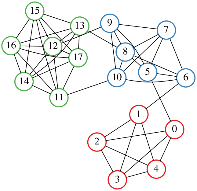
As the connectivity can be considered to indicate the strength of a relationship, we can define hierarchical clustering based on connectivity. This can be visualized using a connectivity dendrogram. Figure 6 shows a graph and its connectivity dendrogram.
The dendrogram of a cut tree can also be easily obtained. Algorithm 5 explains the procedure, which works in time. Given a cut tree, it returns a tree and a function , where each is a subset of the vertices of the original graph, and denotes the connectivity of vertex set . The underlying idea of the algorithm is to look at edges in the cut tree in descending order of their weights and merge the vertex subsets corresponding to both endpoints. In experiments, this algorithm required 0.20 s and 0.30 s with the com-Orkut and indochina-2004 datasets, respectively (excluding the time taken to construct the cut trees).
XI Related Work
Graph Indexing Methods. Because of their importance as back-ends for efficient network analysis, graph indexing methods, i.e., methods that precompute and store some data structures to accelerate certain kinds of computation, have been studied in the data mining community. Examples include methods for the point-to-point shortest-path distance [2, 14, 13], single-source shortest-path distance [35, 10], neighborhood function [30, 11], and personalized pagerank [19]. Cut trees can also be considered as an indexing method for graphs.
Cut-Tree Construction Algorithms. There has been little work on cut-tree construction algorithms, other than the original algorithm of Gomory and Hu [24]. Gusfield’s algorithm [25] is very similar to the Gomory–Hu algorithm, but does not include a contraction step. Though slightly simpler than the Gomory–Hu algorithm, preliminary experiments indicate that Gusfield’s algorithm is almost always slower for networks of interest. Goldberg and Tsioutsiouliklis proposed practical improvements to the Gomory–Hu algorithm for instances arising from optimization problems [23]. Cohen et al. studied thread-level parallelization of the Gomory–Hu algorithm [12].
XII Conclusions
In this paper, we have described a new algorithm for constructing cut trees from massive real-world graphs. Our overall algorithm combines several new techniques covering graph reduction, max-flow acceleration, and min-cut enumeration heuristics. These techniques are tailored to real-world networks, and, as confirmed by our experimental results, the resulting algorithm works surprisingly well. Specifically, our algorithm constructed cut trees for web and social graphs with more than one billion edges, some three orders of magnitude larger than can be handled by previous methods. We also discussed some applications of cut trees to graph data mining.
Repeatability. As the implementations and datasets used in our experiments are available online, our results are completely replicable. The proposed method is available from http://git.io/cut-tree. The previous methods are available from http://www.cs.princeton.edu/~kt/cut-tree/ and https://lemon.cs.elte.hu/trac/lemon. The datasets are available from http://snap.stanford.edu/data and http://law.di.unimi.it/datasets.php.
Acknowledgement. This work was supported by JSPS Grant-in-Aid for Research Activity Startup (No. 15H06828) and JST, PRESTO.
References
- [1] T. Akiba, Y. Iwata, Y. Sameshima, N. Mizuno, and Y. Yano. Cut tree construction from massive graphs. In ICDM, 2016. to appear.
- [2] T. Akiba, Y. Iwata, and Y. Yoshida. Fast exact shortest-path distance queries on large networks by pruned landmark labeling. In SIGMOD, pages 349–360, 2013.
- [3] T. Akiba, Y. Iwata, and Y. Yoshida. Linear-time enumeration of maximal k-edge-connected subgraphs in large networks by random contraction. In CIKM, pages 909–918, 2013.
- [4] Y. Asano, T. Nishizeki, M. Toyoda, and M. Kitsuregawa. Mining communities on the web using a max-flow and a site-oriented framework. IEICE transactions on information and systems, 89(10):2606–2615, 2006.
- [5] J. Bang-Jensen, A. Frank, and B. Jackson. Preserving and increasing local edge-connectivity in mixed graphs. SIAM J. Discrete Math., 8(2):155–178, 1995.
- [6] P. Boldi, M. Rosa, M. Santini, and S. Vigna. Layered label propagation: a multiresolution coordinate-free ordering for compressing social networks. In WWW, pages 587–596, 2011.
- [7] P. Boldi and S. Vigna. The webgraph framework I: compression techniques. In WWW, pages 595–602, 2004.
- [8] M. Borassi and E. Natale. KADABRA is an adaptive algorithm for betweenness via random approximation. CoRR, abs/1604.08553, 2016.
- [9] L. Chang, J. X. Yu, L. Qin, X. Lin, C. Liu, and W. Liang. Efficiently computing k-edge connected components via graph decomposition. In SIGMOD, pages 205–216, 2013.
- [10] J. Cheng, Y. Ke, S. Chu, and C. Cheng. Efficient processing of distance queries in large graphs: A vertex cover approach. In SIGMOD, pages 457–468, 2012.
- [11] E. Cohen. All-distances sketches, revisited: HIP estimators for massive graphs analysis. IEEE TKDE, 27(9):2320–2334, 2015.
- [12] J. Cohen, L. A. Rodrigues, and E. P. Duarte Jr. A parallel implementation of gomory-hu’s cut tree algorithm. In SBAC-PAD, pages 124–131, 2012.
- [13] A. Das Sarma, S. Gollapudi, M. Najork, and R. Panigrahy. A sketch-based distance oracle for web-scale graphs. In WSDM, 2010.
- [14] D. Delling, A. V. Goldberg, T. Pajor, and R. F. Werneck. Robust distance queries on massive networks. In ESA, pages 321–333. 2014.
- [15] B. Dezs, A. Jüttner, and P. Kovács. Lemon - an open source c++ graph template library. Electron. Notes Theor. Comput. Sci., 264(5):23–45, 2011.
- [16] E. A. Dinic. Algorithm for Solution of a Problem of Maximum Flow in a Network with Power Estimation. Soviet Math Doklady, 11:1277–1280, 1970.
- [17] P. Elias, A. Feinstein, and C. E. Shannon. A note on the maximum flow through a network. Information Theory, IRE Transactions on, 2(4):117–119, 1956.
- [18] L. R. Ford and D. R. Fulkerson. Maximal flow through a network. Canadian journal of Mathematics, 8(3):399–404, 1956.
- [19] Y. Fujiwara, M. Nakatsuji, T. Yamamuro, H. Shiokawa, and M. Onizuka. Efficient personalized pagerank with accuracy assurance. In KDD, pages 15–23, 2012.
- [20] A. V. Goldberg. Finding a maximum density subgraph. University of California Berkeley, CA, 1984.
- [21] A. V. Goldberg, S. Hed, H. Kaplan, R. E. Tarjan, and R. F. F. Werneck. Maximum flows by incremental breadth-first search. In Algorithms - ESA 2011 - 19th Annual European Symposium, Saarbrücken, Germany, September 5-9, 2011. Proceedings, pages 457–468, 2011.
- [22] A. V. Goldberg and R. E. Tarjan. A new approach to the maximum-flow problem. J. ACM, 35(4):921–940, 1988.
- [23] A. V. Goldberg and K. Tsioutsiouliklis. Cut tree algorithms: an experimental study. Journal of Algorithms, 38(1):51–83, 2001.
- [24] R. E. Gomory and T. C. Hu. Multi-terminal network flows. Journal of the Society for Industrial and Applied Mathematics, 9(4):551–570, 1961.
- [25] D. Gusfield. Very simple methods for all pairs network flow analysis. SIAM Journal on Computing, 19(1):143–155, 1990.
- [26] J. Hao and J. B. Orlin. A faster algorithm for finding the minimum cut in a directed graph. Journal of Algorithms, 17(3):424–446, 1994.
- [27] J. Leskovec and A. Krevl. SNAP Datasets: Stanford large network dataset collection. http://snap.stanford.edu/data, 2014.
- [28] D. Liben-Nowell and J. Kleinberg. The link-prediction problem for social networks. Journal of the American society for information science and technology, 58(7):1019–1031, 2007.
- [29] J. B. Orlin. Max flows in o(nm) time, or better. In STOC, pages 765–774, 2013.
- [30] C. R. Palmer, P. B. Gibbons, and C. Faloutsos. ANF: A fast and scalable tool for data mining in massive graphs. In KDD, pages 81–90, 2002.
- [31] L. Qin, R.-H. Li, L. Chang, and C. Zhang. Locally densest subgraph discovery. In KDD, pages 965–974, 2015.
- [32] R. E. Tarjan. A note on finding the bridges of a graph. Information Processing Letters, 2(6):160–161, 1974.
- [33] C. Tsourakakis. The k-clique densest subgraph problem. In WWW, pages 1122–1132, 2015.
- [34] R. Zhou, C. Liu, J. X. Yu, W. Liang, B. Chen, and J. Li. Finding maximal -edge-connected subgraphs from a large graph. In EDBT, pages 480–491, 2012.
- [35] A. D. Zhu, X. Xiao, S. Wang, and W. Lin. Efficient single-source shortest path and distance queries on large graphs. In KDD, pages 998–1006, 2013.