Additional authors: Matthias Schubert (LMU Munich, Oettingenstraße 67, 80583 Munich, Germany) schubert@dbs.ifi.lmu.de)
Scenic Routes Now: Efficiently Solving the Time-Dependent Arc Orienteering Problem
This paper extends the Arc Orienteering Problem (AOP) to large road networks with time-dependent travel times and time-dependent value gain, termed Twofold Time-Dependent AOP or 2TD-AOP for short. In its original definition, the NP-hard Orienteering Problem (OP) asks to find a path from a source to a destination maximizing the accumulated value while not exceeding a cost budget. Variations of the OP and AOP have many practical applications such as mobile crowdsourcing tasks (e.g., repairing and maintenance or dispatching field workers), diverse logistics problems (e.g., crowd control or controlling wildfires) as well as several tourist guidance problems (e.g., generating trip recommendations or navigating through theme parks). In the proposed 2TD-AOP, travel times and value functions are assumed to be time-dependent. The dynamic values model, for instance, varying rewards in crowdsourcing tasks or varying urgency levels in damage control tasks. We discuss this novel problem, prove the benefit of time-dependence empirically and present an efficient approximative solution, optimized for fast response systems. Our approach is the first time-dependent variant of the AOP to be evaluated on a large scale, fine-grained, real-world road network. We show that optimal solutions are infeasible and solutions to the static problem are often invalid. We propose an approximate dynamic programming solution which produces valid paths and is orders of magnitude faster than any optimal solution.†† ⋆These authors contributed equally to this work.
1 Introduction
Not long ago, finding the shortest or fastest path in road networks was the core challenge of route planning. Nowadays, challenges are manifold – due to the abundance of sensor data, due to the existence of increasingly complex traffic models and due to the demand for efficient yet convenient solutions. Modern navigation systems often take multiple, sometimes time-dependent, cost criteria into account and solve complex queries in order to increase driver convenience and traffic efficiency. In view of this progress, we propose a novel query with multiple applications. As an extension to the family of Orienteering Problems, we present the Twofold Time-Dependent Arc Orienteering Problem (2TD-AOP).
In its original formulation [22], the Orienteering Problem (OP) requires to find a path from a given source to a given destination abiding by a given cost budget but maximizing the value collected along the way. In most cases, the cost function corresponds to the travel time within the given network. The problem may for instance occur in the field of spatial crowdsourcing [32, 7, 44] where individuals complete advertised tasks in order to collect rewards. A recent popular example of this is the augmented reality game Pokémon Go. A worker who is willing to complete crowdsourced tasks will want to maximize the collected rewards within his chosen time frame. The OP combines the NP-hard Knapsack and Traveling Salesman Problems, hence is NP-hard itself. Numerous variations of the problem have been proposed, for instance, extending it to multiple workers (Team Orienteering Problem) [24] or restricting the collectable values to certain time windows ((Team) Orienteering Problem with Time Windows) [18]. Another variation is the Arc Orienteering Problem (AOP) [2]. In the OP, the value is associated with the vertices of the graph, whereas in the AOP, it is associated with the arcs. Thus, the OP intuitively corresponds to logistic or crowdsourcing tasks, where the value is collected at particular points. The AOP, on the other hand, corresponds to tasks where the value is collected “along the way”. Examples of such tasks are the routes of firefighting planes or the planning of scenic bike trips [42].
Until recently, the AOP has only been answered for networks with static travel times. However, assuming static costs is not reasonable for most real-world scenarios. For road networks, the significance of time-dependence was empirically proven in [13] and substantiated by the incorporation into many navigation services such as Waze11 1 waze.com. In a recent study, Verbeeck et. al [47] first introduced time-dependent travel times but the values have been assumed to be static. In this paper, we propose to incorporate time-dependent values in addition to time-dependent travel times, introducing the 2TD-AOP. As will be shown, results benefit greatly from time-dependent values which model the varying benefit for different times. Without loss of generality, we restrict ourselves to the application of scenic route planning. In this use case, a view of the sea might only be worthwhile during day, whereas a view of the skyline might be particularly worthwhile at night. Thus, the value of a coastline road is high during the day but low at night, while a road passing through downtown may have the opposite values. Other use cases include the aforementioned firefighting planes, collecting street view data or gathering Pokémon Go items.
Consider the example given in Figure 1 which shows different result paths for a scenic path query with the same source and destination. Figure 1(a) shows the time-dependent fastest path according to our algorithm for two departure times. While the path is the same at 11 am and 6 pm, the travel times are not the same (15 and 20 minutes, respectively). In this example, the fastest path does not pass through particularly scenic areas, according to the crowdsourced data set. The other paths pass through such areas, and for particular scenic parts of the respective paths, the hourly value distributions are highlighted. At first glance it is evident that the value functions show great variance over the course of a day. If not allowing for time-dependent values, these functions are commonly averaged, evening out the significant peaks of the distribution.
Suppose a driver is willing to spend 25 minutes for his trip from Hollywood Hotel to the Home Depot north of Griffith Park. Employing an algorithm for the AOP in static networks[38], we obtain the static scenic path displayed in Figure 1(b). The path was computed in a static network derived from our time-dependent network. The static travel time along an arc is set as the average of all travel times along this arc in the time-dependent network. The static scenicness values are derived analogously. The generated result path has a static travel time of 22 minutes which abides by the budget. However, the actual travel time might of course deviate in either direction. For a desired departure at 11 am, the time-dependent travel time coincides with the static time of 22 minutes, but for a desired departure at 6 pm, the time-dependent path takes 37 minutes. Thus, at 6 pm the result path clearly exceeds the budget and is therefore invalid. In a similar way, the averaged scenicness values can deviate from the time-dependent ones. While the static scenic path at 11 am does not exceed the budget, it is not optimal either. Griffith Observatory, which it passes along the way, is a popular sight but particularly scenic during sunset or in the evening. Instead, the best solution at 11 am is displayed in Figure 1(c). This time-dependent scenic path takes 20 minutes and passes a golf course, offering particularly nice views at daytime. The best solution at 6 pm is shown in Figure 1(d). This path takes 22 minutes and passes through central Glendale, a bustling area in the evening and at night.
Taking time-dependence into account when computing AOP paths is crucial. Not only result quality but also result validity depends on it. Our experiments show that every second static solution in a moderately complex settings is invalid. Users benefit considerably from time-dependent travel times as every 2TD-AOP path is valid. Furthermore, results are improved significantly when the values reflect time-dependence as well. Our experiments show that 2TD-AOP paths generate three to four times more value than static solutions. We therefore propose to employ value distribution models whenever possible.
Due to their NP-hardness, static variations of the OP and AOP are usually solved employing metaheuristics. Allowing for time-dependent travel times adds further complexity to the task. Slight modifications of valid solutions may invalidate them. For instance, when taking a minor detour at the beginning of the path, travel times for the rest of the path may change and exceed the budget. Additionally incorporating time-dependent values multiplies this effect. Taking a minor detour at the beginning of a path may result in a change of value and travel time. We propose to solve the 2TD-AOP with a novel dynamic programming approach which makes use of pruning techniques to limit the candidate set and reduce intermediate path computations.


To the best of our knowledge, no previous work has allowed for both travel times and values to be time-dependent. In addition to handling the increased complexity, we require fast response times. We focus on the practicality of the solution where fast response times are crucial and large road network are standard, for instance, in order to meet the requirements of a mobile application. In conclusion, the contributions of this paper are as follows:
- 1.
We motivate and introduce the 2TD-AOP, as a new graph-based routing problem and a Mixed Integer Programming formulation.
- 2.
We present an efficient approximate solution to the 2TD-AOP.
- 3.
We present experiments on a large-scale real-world road network. Our evaluation is the first of this dimension for any time-dependent AOP. We show the value of twofold time-dependence empirically and compare 2TD-AOP solutions to static solutions as well as to optimal results.
The remainder of this paper is organized as follows. In Section 2 we give an overview of research relevant to our work. In Section 3 the 2TD-AOP is formally defined and formulated as an Mixed Integer Programming. In Section 4 we lay the theoretical foundation for our algorithm which is described in Sections 5 and 6. Subsequently, our algorithm is evaluated in Section 7. A conclusion is provided in Section 8.
2 Related Work
We divide research relevant to this work into three groups. First, we review research on how to attain profit values from data in general and crowdsourced content in particular. Next, we briefly introduce related research from the database community such as the Trip Planning Query (TPQ). These problems have a similar field of application but are not congruent to the problem discussed in this paper. Finally, we present research on the family of OPs which mostly stems from the field of Operations Research. We give an overview of solutions to the static and time-dependent OP and AOP.
2.1 Attaining Value Functions
An important aspect of the OP/AOP is how to attain the value functions, in particular when aiming to solve a time-dependent instance. Most works from the field of Operations Research rely on specific bench mark data sets, some synthetic, others real. The authors of [42], for instance, evaluate their approach to cycle trip planning on real-world tourist data from Flanders, Belgium. The authors of [25] use data from Chinese theme parks. Relying on specifically recorded data like the above has two major drawbacks. First, expert knowledge or an official mandate may be required to attain the data. Second, the data may not be available globally. As this approach usually lacks scalability, there exist advances to mine this knowledge from freely available data.
Crowdsourced data is a rich source of information. It is for instance used for general POI recommendation [27], for categorization [5], for popularity estimation [3], for determining opening hours or visiting times [26], for determining duration of stay [9] or for determining spatial connectivity [41]. The most common data sources for these purposes are Foursquare, Yelp, Twitter, Flickr22 2 foursquare.com, yelp.com, twitter.com, flickr.com or the inoperative but oft-cited Gowalla. When interested in how to attain value functions from the raw data, we refer the reader to the respective works. In the context of this paper, we assume the values to be given. For our experimental evaluation, we rely on Flickr data, details are given in Section 7.
2.2 TPQ and Related Queries
The most related query in the database community is the TPQ [8] (alternatively, Route Planning Query [6] or Route Search Query [35]). In this problem setting, the user specifies a different POI categories, e.g., “ATM”, “restaurant”, “florist”, “cinema”. The result of a TPQ is the fastest path from a given source to a given destination visiting exactly one instance of each resource. The TPQ is NP-hard because in the case that each category occurs exactly once, the TPQ degenerates to the Traveling Salesman Problem. There exist several variations, for instance introducing order constraints [33, 30] or modeling the fulfillment at a location probabilistically or time-dependent [31, 29, 11]. Solutions to this problem include full enumeration [11], heuristics [6, 33, 11], or backtracking and branch-and-bound approaches [29]. Partially time-dependent variations of these queries exist, however, most of the research pertains to static networks. Most importantly, albeit related, the problem settings of the OP/AOP and the TPQ are not congruent.
2.3 OP and AOP
Blueprint for the OP was the family of orienteering sports where efficient navigation from checkpoint to checkpoint is the goal [22]. Alternative names for the OP include the Selective Traveling Salesman Problem [34] or the Traveling Salesman Problem with Profits [14]. The OP is executed on a graph whose arc weights represent traversal costs and whose vertices may yield certain value. Given a source, a destination and a cost budget, the output of an OP is the path with maximum value among all paths not exceeding the budget. In the variation referred to as AOP or Privatized Rural Postman Problem [1], the profit is not assigned to vertices but to arcs, while the rest is as before. Extensive surveys on these problems and their numerous variants are given in [46, 24, 2] (or from the perspective of the related Tourist Trip Design Problem in [18]).
Although NP-hard [22], exact solutions to the OP exist [34, 40, 14]. Most solutions, however, are approximative. While in older research specific heuristic approaches were proposed [45, 23, 4], the trend shifted towards algorithms following particular meta-heuristics such as Tabu Search [21], Genetic Algorithms [43] or Ant Colony Algorithms [37]. This holds similarly for the AOP where exact algorithms [10, 48] are rare but available. Generating approximative solutions is the standard approach [20], most effectively following the meta-heuristics Iterative Local Search (ILS) [48] and Greedy Randomized Adaptive Search Procedure (GRASP) [42, 38]. Recently, ILS and GRASP have been improved to solve the AOP on large scale real-world road networks in near-interactive time [38].
Introduced in [15], the OP with time-dependent (TD-OP) costs has gained attention recently [25, 17, 19, 47, 36]. Typical applications for the TD-OP include electronic tourist guides [17, 16] or routing in theme parks [25]. The time-dependent AOP (TD-AOP) as presented in [47] is not directly linked to an application but a time-dependent extension of the authors’ cycle trip planning application [48] is imaginable.
The above works are all evaluated on small graphs (with the exception of [38]) with no more than a couple of hundred vertices. Most arcs in these graphs connect two non-zero value vertices. For instance, in the theme park data set of [25], vertices correspond to attractions and the arcs are fastest paths between them. The travel times and the values are derived from user data of the theme parks and their attractions. Similarly, [19] and the demonstration paper [16] are evaluated on data sets consisting of Points of Interest (POIs) and fastest paths connecting these POIs (by walking or by public transportation). When considering real-world road networks, this is not feasible. A moderate-sized network usually contains over one million vertices and two to three million arcs. In a time-dependent network, there usually exist numerous fastest paths from a given vertex to another, depending on the departure time. Hence, introducing shortcuts for precomputed fastest paths as in the approaches above is not possible. This is particularly the case, if the travel times are not statistically inferred but real-time, i.e., depending on live information, as is the case in the network of our evaluation.
The most closely related problem to the 2TD-AOP is the TD-AOP with time-dependent costs and static value. Verbeeck et. al recently proposed to solve this problem with an Ant Colony System algorithm [47]. Evaluated on specific benchmark instances with at most 100 vertices, the proposed approach finds near-optimal to optimal solutions within an average runtime of one second. The complex solver has excessive time requirements (“often more than 100 hours” [47]) to generate optimal solutions on these benchmark instances of the TD-AOP. In comparison, we increase complexity of the problem in two ways. First, by including time-dependent value functions 2TD-AOP adds another dimension of time-dependence to the problem. Second, we aim to solve the problem on large-scale real-world road networks with hundred thousands of vertices. Established solutions to related problems like the TD-AOP or the TD-OP rely on metaheuristics such as the Ant Colony System [47], Iterative Local Search [48] or Greedy Randomized Adaptive Search Procedure [42, 38]). Instead, we propose a heuristic dynamic programming approach.
3 Problem Definition
We model the road network as a graph , where denotes the set of vertices (or nodes), denotes the set of directed arcs (or edges), and (with the same domains) denote the non-negative functions mapping each arc onto its respective value and the travel time, respectively
For the representation of the time-dependent travel time along an arc, we use a piecewise constant function with equal step width . In the following, we refer to the intervals where travel time is constant as time windows and denote the -th time window by , where for some maximum time window .
A consecutive set of arcs which visits no arc twice is called a path. A path from source to destination departing at is denoted by where is the source vertex and the destination vertex. In the remainder of this paper, we simplify notation for the sake of clarity. We omit the double indexes and denote a path by
For each query, we denote source and destination by and , respectively. The travel time of a path is defined as , where denotes the time of arrival at (and departure from) vertex . is dependent on the travel times along the preceding arcs and is defined iteratively:
The value of a path is defined as:
For a given source , destination , and departure time , we denote the set of all paths from to starting at by .
The input for the 2TD-AOP is a graph , a source vertex , a destination vertex , a departure time , and a time budget . When speaking of a query, we mean the set of these inputs. The optimal path to a 2TD-AOP query is the path maximizing the collected value among all feasible paths. Both notions are defined in the following.
Definition 1 (feasible path)
Given a query, we call any path departing from at and arriving at no later than (i.e., ) a feasible path.
Definition 2 (optimal path)
Given a query, among all feasible paths, we call one with maximum value an optimal path.
Extending the work in [46, 47], we give a mixed integer programming (MIP) formulation of the problem. We introduce the following two decision variables: is a binary decision variable which equals if the result path enters the arc in time window and if the arc is not traversed at all or entered in a different time window. is a continuous decision variable containing the time of departure at when entering the arc in time window . Again, it is if the arc is not traversed at all or entered in a different time window.
| (1a) | ||||
| (1b) | ||||
| (1c) | ||||
| (1d) | ||||
| (1e) | ||||
| (1f) | ||||
| (1g) | ||||
| (1h) | ||||
Equation 1a gives the objective function while Equation 1b gives the budget constraint. Note that due to the time-dependent nature of the problem, all time windows have to be taken into account when summing the collected value and cost. Remember, however, that is a binary decision variable which for each arc can at most once be equal to , as each vertex (and thereby also each arc) is at most visited once. This is expressed in Constraint 1c. Constraint 1d ensures that the result path starts at the source and ends at the destination. Next, Constraint 1e ensures that the departure time at each arc is the departure time at its predecessor plus the travel time within the corresponding time window. Note that this condition implicitly forbids “waiting” at vertices. Finally, Constraints 1f and 1g determine the domain of the decision variables and Constraint 1h ensures that the path departs from the source at .
4 Solving the 2TD-AOP
In this section, we present terminology and insights essential to our solution of the 2TD-AOP.
Definition 3 (earliest arrival)
Given a graph , a source , a vertex , and a departure time , we define the earliest arrival (time) for reaching from when departing at , denoted by ( for short), as follows:
Definition 4 (latest departure)
Given a graph , a destination , a vertex , and a latest arrival time , we define the latest departure (time) for reaching from no later than , denoted by ( for short), as follows:
i.e., the latest departure time among all feasible paths w.r.t. , , and .
Definition 5 (forward-reachable)
Given a graph , a source , a departure time , and a time budget , we refer to the vertices reachable within the budget from (when departing at ) as forward-reachable vertices, denoted by (FWR for short if and are clear from context).
Definition 6 (backward-reachable)
Given a graph , a destination , a departure time , and a time budget , we refer to the vertices from which the destination can be reached within the budget when departing no earlier than as backward-reachable vertices, denoted by (BWR for short).


Intuitively, all forward-reachable vertices lie in a quasi-circular region around the source. This region is similar to the circular expansion of a Dijkstra-search. The difference is that in this case the cost criterion is time-dependent travel time. Analogously, all backward-reachable vertices lie in a quasi-circular region around the destination. This graphical intuition is visualized in Figure 2(a). If the destination is not forward-reachable from the source (and/or vice versa), then the query has no answer.
Our solution to the 2TD-AOP is based on an extension of this observation: For an arc to be part of a feasible path, it is a necessary condition that is forward-reachable from the source and is backward-reachable from the destination . Hence, if an arc is not contained in the intersection of the forward-reachability region and the backward-reachability region, it cannot be part of a feasible path. This property will be proved later on. In our solution to the 2TD-AOP, arcs which increase the value are recursively inserted until the budget is exhausted. With every insertion of an arc, the overall travel time of the path increases. Hence, the reachability regions iteratively contract until no more arcs can be inserted. Before we detail this approach in the next section, let us explain the above definitions and their computation with an example.


The definitions are visualized in Figure 3. Figure 3(a) shows a graph with source and destination . Departure time is , and let the time budget . The time-dependent travel times along the arcs are visualized in Figure 3(b). The arcs in Figure 3(a) are labeled with letters which correspond to the travel time functions in Figure 3(b). Figure 3(c) shows the earliest arrivals and latest departures according to this query. If not indicated otherwise, vertices are forward-reachable as well as backward-reachable. The earliest arrivals are computed as in the definition. For example, , implying that the fastest path from at arrives at at time .
Consider the following path:
Since there is no shorter path from to , is not FWR within the given budget. From there are two feasible paths to :
Which of the two constitutes the optimal path depends on the time-dependent value functions and will be discussed later on.
Let us turn to the computation of the latest departures. For example, , implying that in order to arrive at no later than , one must depart at time . Now, consider : the only path to the destination follows the arc . Departing at time results in exceeding the budget, since . The same holds for time . However, when departing at , then , resulting in an arrival within the budget . Hence, in order to compute the latest departure time of a vertex a linear scan among the time windows might be required. Note that the difference between “at time ” and “before time ” is infinitesimal. In theory we set the latest departure at to , in practice, we adjust it by a sufficiently small number. Let us note that this special case only occurs if the latest departure at a vertex by chance coincides with the border between two time windows which is very unlikely in practice. Finally, we prove that in order to compute all feasible paths it suffices to consider the vertices which are forward-reachable and backward-reachable.
Lemma 1
All vertices along all feasible paths are contained in the intersection of the sets of forward-reachable and backward-reachable vertices.
Proof 4.1.
Suppose there exists a feasible path visiting a vertex . Case 1: , this implies , meaning that the subpath from to already exceeds the budget, which contradicts the assumption that is feasible. Case 2: Analogously, if , then , hence cannot be a feasible path.
5 Computing Reachability
Having clarified the importance of the sets of reachable vertices, we will now go into detail on their computation. Both sets are generated by expansions around source and destination with “time-radius ”. By the above lemma, all vertices along all feasible paths are contained in the intersection of the two reachability regions.
In order to compute the set of forward-reachable vertices (for a given source , departure time , and a time budget ), we perform a modified time-dependent all-target Dijkstra search starting at at time , called FWR and illustrated in Algorithm 1. All earliest arrival times are initialized as except for the source for which it is . Additional to a result set containing all visited vertices, we maintain a priority queue containing vertices sorted in ascending order by the earliest arrival time of each vertex. In every iteration, the top element of the queue is removed. In the for-loop spanning lines 8-21, the outgoing arcs of the current vertex are explored. In line 9, the travel time from to its neighbor is added to the earliest arrival time at . If this value does not exceed the budget , is forward-reachable. If was previously not visited, is set accordingly and is added to the queue as well as the result set. If was previously visited and the updated earliest arrival time is better than the previous, it is updated accordingly. Note that once a vertex has been dequeued, the label is final. This is equivalent to the Dijkstra property which ensures that any processed vertex is reached by the shortest path, in this case the fastest time-dependent path. Finally, the result set contains all vertices reachable from the source within the budget.
The set of backward-reachable vertices is computed in a similar fashion but slightly more complicated. The procedure is presented in Algorithm 2 and called BWR. In addition to the result set containing all backward-reachable vertices, we maintain a queue of vertices sorted in descending order by . Initially, the latest departure at the destination is set to the latest possible arrival time, . The algorithm operates backwards from the destination, following incoming arcs which are explored in the for-loop spanning lines 8-25. As was illustrated in the above example (Figure 3), in order to find the latest departure, it is required to linearly scan the time windows. When exploring an incoming arc from to , is initially set to the latest time window not exceeding the latest departure from . If at the travel time from to is too high (i.e., cannot be reached in time for its latest departure), is decremented implying an earlier departure at but possibly also a different travel time along the arc. Note the in line 13, corresponding to the aforementioned special case that for some . In this case, is decreased by a small number in order to avoid computational errors which may occur at time window boundaries. Once a valid latest departure time for is found, is set accordingly. If was previously visited, is only set if it is later than the previous latest departure. Upon termination, all vertices which are backward-reachable from the destination within the given budget are in the result set and labeled with their respective latest departure.
6 Computing Solutions


Due to the NP-hardness of the problem, we forgo giving an optimal solution as it would not meet our requirements of providing solutions on large graphs in efficient time. Instead, we propose a heuristic solution to the
Problem 1.
. So far no other solution to the
Problem 2.
exists. Our dynamic programming solution recursively fills gaps with arcs in order to improve the value while not exceeding the budget. Upon initialization, the set of arcs arcs is empty, the set of gaps gaps contains , i.e., the gap given by the query. Assume that in the first iteration the arc is inserted. Then arcs holds the new arc and gaps holds two new gaps, and . Into the new gaps, further arcs will be inserted. This procedure is repeated until the budget is exhausted. Hence, the
Problem 3.
is solved in a divide-and-conquer manner by recursive insertions. We therefore refer to the algorithm, pseudo-coded in Algorithm 3, as RecInsert.
We will now explain in detail how the algorithm proceeds. The two sorted lists gaps and arcs hold two-tuples of vertices. gaps holds pairs between which arcs are to be inserted, and arcs holds the converse information, i.e., the arcs already inserted. With every insertion, the budget is decreased by the duration of the detour that has to be taken to insert the new arc. However, this detour is not explicitly computed as a path. Instead, it is implicitly derived from the information generated during FWR and BWR. The earliest arrivals and latest departures of every gap allow to decide whether an arc can be feasibly inserted, i.e., without exceeding the budget. This is crucial to the performance of our algorithm. Established metaheuristics usually compute, improve and perturb solutions. Starting from an initial path, promising arcs are (usually randomly) inserted and under certain conditions (usually randomly) deleted, to avoid local value maxima. Instead, RecInsert holds a sorted list of arcs which may be feasible inserted into a path. The actual paths between these arcs, however, are not computed until the budget is exhausted.
The arc which is to be inserted into a gap is chosen based on a heuristic. Among all arcs which can be feasibly inserted, the arc is selected which yields the best ratio of value to detour. This step is performed in the for-loop spanning lines 9 to 19. As established, all feasibly insertable arcs lie in the intersection of the reachability regions. The intersection is performed in line 8, therefore the set in line 9 comprises all arcs which can be feasibly inserted. In line 10, the detour incurred by inserting an arc is expressed as a decrease in budget. Assume that for the gap between and , the arc is examined for insertion. is the earliest arrival at coming from , and is the latest departure from to reach “in time” (depending on the recursive budget ). Thus, corresponds to the budget that would remain when taking the detour of traveling from to , then along (at time ) and from to . Hence, if inserting , the budget will be set to . In line 11, the gain in value is estimated. Note that the actual gain in value may be higher (due to other arcs along the path). However, in order to compute the actual gain in value, the fastest paths to and from each arc would have to be computed. Also, the value of all succeeding arcs would have to be reassessed. For the sake of efficiency, we therefore only estimate the value as proposed. The estimated gain in value divided by the decrease in budget yields the ratio by which we evaluate the arcs. The arc with the best ratio is inserted, i.e., the arc is added to arcs as a pair of vertices, and two pairs of vertices are added to gaps (the gaps left and right of the new arc). As long as at least one arc qualifies for insertion, RecInsert is recursively called with the extended sets gaps and arcs and the reduced budget . If no arc can be inserted (into any of the gaps), the time-dependent fastest paths for all gaps are computed and the concatenation is returned which constitutes our approximate solution to the
Problem 4.
.
6.1 Pruning Strategies
Let us discuss three variations which are omitted in the algorithm description for reasons of brevity. , it is recommended to employ a simple forward estimation during FWR. , it is recommended to compute the intersection of FWRi and BWRj during computation of BWRj. , it is possible to make the recursive call with a restricted portion of the graph. Variations and are based on the following observation. The sets FWRi and BWRj are not needed separately, only their intersection is needed. Therefore, we may exclude vertices which are not contained in the intersection during computation of the respective sets.
Regarding : We propose to employ a simple forward estimation for pruning. If information about the speed limits is available, the following lower bound can be used with negligible overhead. During FWR, in line 10, the if-clause may be tightened:
where is the Euclidean distance from to the destination and is maximum speed in the given network. If traveling from to the destination at maximum speed exceeds the budget, so will any actual path. Any such vertex cannot be forward-reachable. Figure 4(a) illustrates the effect of this pruning strategy yielding a trimmed forward-reachability region. We refer to this pruning strategy as FWEST pruning. At marginal computational cost, FWEST yields a perceptible reduction in candidates. In our experiments, over 15% of vertices are pruned during FWR using this approach. Of course, the method holds analogously for BWR and can equally be applied. However, during BWR it is recommended to use the following pruning technique which is superior but exclusive to BWR.
Regarding : One may use that for all vertices in the intersection holds . This follows from the definition:
where denotes the fastest path from to at . Hence, the if-clause in line 14 of BWR can be tightened to . In this case, the simple forward estimation cannot be applied because
By construction, is based on an actual path expansion and therefore serves as a tighter bound than any estimation. We refer to this pruning strategy as EALD pruning. Figure 4(b) illustrates the effect of this pruning strategy, where the vertices which are not forward-reachable are not visited during BWR. Thus, instead of computing both reachability regions separately and subsequently their intersection, the information of FWR may be used in BWR. This limits the search space and implicitly computes the intersection. Every vertex in the intersection will be visited during BWR. Unvisited vertices are either not forward-reachable or backward-reachable. The effect of this pruning strategy is remarkable. Particularly when taking into account that it causes no computational overhead. When visiting a vertex during BWR, it suffices to retrieve its earliest arrival to decide if it qualifiies for pruning.
Regarding : It is possible but not necessarily recommended to issue the recursive call of RecInsert with a restricted portion of the graph. As established in Lemma 1, all vertices along feasible paths are in the intersection of the reachability regions. This property holds recursively. For instance, consider the insertion of a first arc into the initial gap . In the next recursion, two gaps will be examined, and , as illustrated in Figure 2(b). Consider the first gap , the respective reachability regions (forward from and backward from ) are contained in the original reachability regions (forward from and backward from . Moreover, the intersection is contained in the original intersection. Thus, it suffices to input a restricted graph into the next recursion:
Albeit correct, actually computing the union of these graphs may cause more computational overhead than it saves. In our experiments, computing the restricted graph has not proved efficient. We input the initial intersection of and into all recursions as it restricts the graph significantly while not requiring costly unions of graphs.
Let us note that Gunawan et. al use very similar terminology in their approach to solving the TD-OP [25]. However, there are significant differences to the approach presented here. First, the authors solve TD-OP where travel times are time-dependent but values are assumed to be static and associated with vertices. Second, the authors propose a different algorithmic approach. While also using the terms earliest arrival and latest departure, they are computed differently and for different purposes. Given a specific path, a routine called ForwardPropagation computes the earliest arrival times at all vertices along the path. Analogously, BackwardPropagation computes the latest departures. In comparison, our FWR and BWR procedures compute earliest arrivals and latest departures for all vertices which are feasibly insertable into a given gap. From this information, the travel time for a detour to any feasibly insertable arc is derived. This is done without explicit path computation. While we use dynamic programming in a divide-and-conquer manner, Gunawan et. al follow an Iterative Local Search (optionally Variable Neighbor Descent) approach. where actual paths are computed, improved and perturbed. In their experiments, they produce near-optimal to optimal solutions with a maximum runtime of one second. Their approach is evaluated on small data sets with at most 40 vertices and 40 time windows. The arcs correspond to precomputed fastest paths. This restrictive scenario is not comparable to the use case we are modeling in this paper where fast response times are required for a more complex problem on graphs which are orders of magnitude larger.

7 Experimental Evaluation
We evaluate our solution to the
Problem 5.
on a time-dependent road network of Los Angeles, CA, USA [13, 28] which contains about 500K vertices and 1M arcs. The travel time functions in this network are derived from large-scale and high-resolution (both spatial and temporal) sensor data (both live and historic) from different transportation authorities in California. The step length of the piecewise constant travel time functions is 5 minutes, details can be found in [12]. Based on the data, streets are uncongested between 9 pm and 6 am. Therefore, travel times are assumed to be static in this interval.
| peak interval | # of arcs | % of all arcs |
|---|---|---|
| 8:00 am - 12:00 pm | 6,238 | 0.57% |
| 12:00 pm - 4:00 pm | 7,366 | 0.67% |
| 4:00 pm - 8:00 pm | 5,851 | 0.53% |
| 8:00 pm - 8:00 am | 6,417 | 0.59% |
| all intervals | 25,872 | 2.38% |
The time-dependent value functions are derived from a geo-tagged set of Flickr photos [39] consisting of 217,391 photos in the area of Los Angeles. For each arc the value is the number of photos which have as their nearest arc (but not further than one kilometer) and which were taken in the hour-interval that contains . Hence, the step length of the piecewise constant value functions is 60 minutes. Figure 5 illustrates the size of the network and the distribution of non-zero value arcs. Each arc which has positive value in some time window is visualized as a colored shape. Shape and color depend on the time interval in which the value of the arc is the highest. For example, an arc with highest value between 6:00 and 7:00 pm will be displayed as red circle. Table 1 presents the absolute and relative numbers of arcs with non-zero value. The number of photos taken during the day is about three times higher than during night.
For the following experiments, we arrange paths into six time buckets. We randomly draw source and destination vertices from the network and compute the respective time-dependent fastest paths using [12]. If the travel time of a path is minutes , its source and destination pair is assigned to the minutes time bucket for . Each time bucket consists of twenty source and destination pairs. Since travel times are empirically static at night and value peaks less frequent at night, we randomly sample departure times from the interval 8 am to 8 pm. We make a case for twofold time-dependence, therefore, a network with significant time-dependent impact on travel time and value is essential. Our standard experimental setting has the following inputs. Standard time bucket is 20 minutes, standard query budget is 200% (i.e., 40 minutes), and departure times are randomly drawn from 8 am to 8 pm. Deviating values are explicitly mentioned. For each query, the departure time is the same across time-dependent algorithms.
We omit providing results of the MIP formulation given in Section 3 generated by a complex solver. This is due to the exorbitant computatial requirements. Even for small instances with at most 100 vertices, solving a less complex MIP often requires days [47, 25]. However, for comparison, we compute optimal solutions with a custom dynamic programming method.

7.1 Experimental Results
In a first set of experiments, we compare the value of result paths generated by different algorithms taking varying degrees of information into account. As in the introductory example, we compare
Problem 6.
paths computed by RecInsert with static scenic paths and to time-dependent fastest paths. For the static scenic paths, we use the AOP solution presented in [38] which employs an Iterative Local Search approach combined with spatial pruning techniques. In accordance with the metaheuristic, it generates an initial solution which is subsequently improved by inserted arcs and perturbed by deleting arcs. The insertion follows a heuristic, the deletion is pseudo-random. We refer to solutions created by this approach as AOP paths and call this algorithm AOP-ILS. It operates on a network with static travel time and static value which are both derived by averaging the respective time-dependent functions. Note that AOP queries are given the same time budget but require no departure time. For the time-dependent fastest paths, we use the solution proposed in [12] which relies on hierarchical routing and forward estimations to conduct efficient bidirectional path computation. We refer to the results as Fastest paths. The results generated by RecInsert are referred to as 2TD-AOP paths.
The values and travel times of all paths are computed w.r.t. the time-dependent functions. For a given path, the value and travel time are the sum of value and travel time of each arc along the path upon arrival. Recall the introductory example in Figure 1. For varying departure times in this example, the result values are displayed in Figure 6. As mentioned in the example, it is possible that paths computed in the static network are invalid in the time-dependent network. This is the case if the time-dependent travel time exceeds the budget. Static paths where this is the case are marked with a red cross. For instance, when departing at 6 pm, the time-dependent travel time is 37 minutes, exceeding the budget of 25 minutes by almost 50%.

Figure 7 shows the value for the different approaches. Fastest paths serve a baseline which shows how much value can be attained “by chance” as it does not optimize for value. Indeed, Fastest paths collect negligible value. Since the non-zero value arcs are rather scarce, this is not surprising. 2TD-AOP and AOP, in contrast, optimize for value. It can be observed that on average 2TD-AOP generates three times the value of AOP. This gap widens for increasing path length.
Figure 8 illuminates the effect of the query budget. We observe that with increasing budget, 2TD-AOP paths generate significantly more value than AOP solutions. This is particularly noteworthy as the problem becomes more complex with increasing budget. A higher budget allows for greater detours which in turn increases the search space. RecInsert leverages this effect to create better solutions. In contrast, AOP results barely improve. Therefore, albeit increasing complexity, twofold time-dependence is able to enhance results considerably.
As mentioned before, static paths may prove invalid when considering time-dependent travel time. Given the departure times of 2TD-AOP and Fastest, we determine the portion of static paths that prove invalid when evaluated in the time-dependent network. The percentage of AOP which are invalid increases from 25% to almost 50% across the increasing time buckets. Note that Figures 7 and 8 show the values of all AOP paths, both valid and invalid, as there is no significant difference. However, taking into account the percentage of invalid results and the low overall value, static results cannot compete with twofold time-dependent results.
The proposed pruning strategies are evaluated in Figure 9. It shows the percentage of visited vertices relative to the number of visited vertices when employing no pruning technique. In this case, all vertices in FWR and BWR have to be visited. In Section 6 we propose two pruning techniques for RecInsert, FWEST and EALD. FWEST is a basic forward estimation which can be applied during FWR and BWR. EALD uses the information generated during FWR to limit the search space of BWR and can only be applied during BWR. During BWR, EALD is superior to FWEST. Hence, when both are available, FWEST is obsolete during BWR. In the experiments displayed in Figure 9, we show the effect of each pruning technique separately as well as of both pruning techniques combined. When only employing FWEST (during both FWR and BWR), almost 40% of the vertices can be pruned. Although EALD can only be applied during BWR, it prunes about 45% of the vertices. As FWEST causes negligible and EALD causes no computational overhead, it is recommended to employ both. Combining both approaches, 65% of all vertices in FWR and BWR can be pruned.


In terms of general complexity, the
Problem 7.
is considerably more intricate than the AOP. While both problems are NP-hard, twofold time-dependence incurs additional complexity. This is mainly due to two aspects. First, fastest path computation is more efficient in static networks. Second, in order to assess the time-dependent value of an arc, it does not suffice to simply retrieve its value. The time frame of arrival has to be considered. In light of these challenges, the efficiency of RecInsert is all the more surprising. Figure 10 shows the processing times of RecInsert solving the 2TD-AOP and AOP-ILS solving the AOP. 2TD-AOP solutions can be computed in less than twice the processing time of AOP solution, usually under two seconds. The increase in processing time for both algorithms in linear in the travel time of the fastest path. Taking the result quality into consideration, the additional processing time of RecInsert compensates for the often invalid AOP paths with less value. It should also be noted that in an application where fixed response times are required, it would be possible to terminate the arc insertion in RecInsert prematurely and construct an early result path.
Finally, we compare
Problem 8.
and AOP paths to optimal solutions in terms of their value. The optimal solutions are computed with a custom dynamic programming approach using a depth-first search and several pruning techniques. Any naïve algorithm, much like a complex solver, would not be able to compute solutions in feasible time. Our custom approach takes between 3 to 6 hours per optimal path computation for the standard query setting. Even for minor instances where the fastest path takes 5 minutes and the budget is 10 minutes, computing an optimal solution takes between 1 and 2 hours. Hence, generating optimal solutions to the
Problem 9.
is infeasible. This is irrespective of the application. Users will not tolerate response times in the hours, and precomputation is not possible in time-dependent networks. Figure 11 compares the accuracy of
Problem 10.
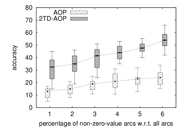
paths generated by RecInsert and of AOP paths generated by AOP-ILS. Values are shown relative to values of optimal paths. Figure 11 also illustrates the effect that the density of non-zero value arcs has on the result. The value is given relative to the optimal value for different networks when varying the percentage of non-zero value arcs. In our original network about 2% of the arcs have non-zero value during some time window. For this experiment, we randomly copied value functions to arcs with zero value to increase density to 4%, 6%, 8% and 10% of all arcs. Also, we set some of the value functions to zero, generating a network with 1% value arcs. As both algorithms follow a heuristic during arc insertion, they are more easily sidetracked in a network with many value arcs. When the density of value arcs decreases, however, the employed heuristics prove effective. In this case, RecInsert result paths attain between 50% and 60% accuracy. The static solutions, in contrast, hardly exceed 25%. Again, this establishes the superiority of
Problem 11.
over AOP solutions. While computing an optimal solution takes up to 6 hours, RecInsert takes about 2 seconds. Thus, RecInsert produces paths with about 50% accuracy in the processing time. As the
Problem 12.
cannot be expected to be solved optimally in efficient time, RecInsert yields a promising trade-off.
In conclusion, our experimental evaluation has established the importance of twofold time-dependence. Solutions to the
Problem 13.
are superior to solutions to the static AOP. For increasingly complex query settings, this trend is intensified. Furthermore, RecInsert computes solutions that achieve 50% accuracy compared to optimal results within seconds. The efficiency can essentially be attributed to the pruning techniques employed in RecInsert. As of now, no time-dependent AOP has been evaluated on large-scale real-world road networks. We prove that even in such networks, the higly complex
Problem 14.
can be feasibly solved.
8 Conclusions
In this paper, we present the Twofold Time-Dependent Arc Orienteering Problem (
Problem 15.
) a novel extension of the family of Orienteering Problems (OP). In this family of NP-hard graph problems, the goal is to find a path from a given source to a given destination within a given time budget which, additionally, maximizes the value collected along the way. In comparison to static versions of this problem,
Problem 16.
allows for travel times and value functions to be time-dependent. The incorporation of time-dependent values is a novel extension which has not been studied yet. The importance of time-dependent values is showcased and experimentally substantiated. Due to the NP-hardness and the twofold time-dependence, we provide a heuristic approximation for solving the
Problem 17.
. Our approach is evaluated on a large-scale real-world road network. Thus far, no time-dependent variant of the AOP has been evaluated on a network of this dimension. Twofold time-dependent results gain significantly more value than static results, showing the importance of twofold time-dependence empirically. Our algorithm produces result paths with 50% accuracy where no optimal solution is feasible.
References
- [1] J. Aráoz, E. Fernández, and C. Zoltan. Privatized rural postman problems. Computers & operations research, 33(12):3432–3449, 2006.
- [2] C. Archetti and M. G. Speranza. Arc routing problems with profits. Arc Routing: Problems, Methods, and Applications, MOS-SIAM Series on Optimization, pages 257–284, 2013.
- [3] I. Brilhante, J. A. Macedo, F. M. Nardini, R. Perego, and C. Renso. Where shall we go today?: Planning touristic tours with tripbuilder. In Proceedings of the 22Nd ACM International Conference on Information & Knowledge Management, CIKM ’13, pages 757–762, New York, NY, USA, 2013. ACM.
- [4] I.-M. Chao, B. L. Golden, and E. A. Wasil. A fast and effective heuristic for the orienteering problem. European Journal of Operational Research, 88(3):475–489, 1996.
- [5] C. Chen, D. Zhang, B. Guo, X. Ma, G. Pan, and Z. Wu. Tripplanner: Personalized trip planning leveraging heterogeneous crowdsourced digital footprints. IEEE Transactions on Intelligent Transportation Systems, 16(3):1259–1273, 2015.
- [6] H. Chen, W.-S. Ku, M.-T. Sun, and R. Zimmermann. The multi-rule partial sequenced route query. In Proceedings of the 16th ACM SIGSPATIAL International Conference on Advances in Geographic Information Systems (ACMGIS’08), pages 10:1–10:10, 2008.
- [7] Z. Chen, R. Fu, Z. Zhao, Z. Liu, L. Xia, L. Chen, P. Cheng, C. C. Cao, Y. Tong, and C. J. Zhang. gmission: A general spatial crowdsourcing platform. Proceedings of the VLDB Endowment, 7(13):1629–1632, 2014.
- [8] D. Cheng, M. Hadjieleftheriou, G. Kollios, F. Li, and S.-H. Teng. On trip planning queries in spatial databases. In Proceedings of the 9th International Conference on Advances in Spatial and Temporal Databases (SSTD’05), pages 273–290, 2005.
- [9] M. De Choudhury, M. Feldman, S. Amer-Yahia, N. Golbandi, R. Lempel, and C. Yu. Automatic construction of travel itineraries using social breadcrumbs. In Proceedings of the 21st ACM Conference on Hypertext and Hypermedia, HT ’10, pages 35–44, New York, NY, USA, 2010. ACM.
- [10] R. Deitch and S. P. Ladany. The one-period bus touring problem: Solved by an effective heuristic for the orienteering tour problem and improvement algorithm. European Journal of Operational Research, 127(1):69–77, 2000.
- [11] A. Delis, V. Efstathiou, and V. Verroios. Reaching available public parking spaces in urban environments using ad hoc networking. In Proceedings of the 12th International Conference on Mobile Data Management (MDM’11), pages 141–151, 2011.
- [12] U. Demiryurek, F. Banaei-Kashani, C. Shahabi, and A. Ranganathan. Online computation of fastest path in time-dependent spatial networks. In International Symposium on Spatial and Temporal Databases, pages 92–111. Springer, 2011.
- [13] U. Demiryurek, F. B. Kashani, and C. Shahabi. A case for time-dependent shortest path computation in spatial networks. In 18th ACM SIGSPATIAL International Symposium on Advances in Geographic Information Systems, ACM-GIS 2010, November 3-5, 2010, San Jose, CA, USA, Proceedings, pages 474–477, 2010.
- [14] D. Feillet, P. Dejax, and M. Gendreau. Traveling salesman problems with profits. Transportation science, 39(2):188–205, 2005.
- [15] F. V. Fomin and A. Lingas. Approximation algorithms for time-dependent orienteering. Information Processing Letters, 83(2):57–62, 2002.
- [16] A. García, O. Arbelaitz, M. T. Linaza, P. Vansteenwegen, and W. Souffriau. Personalized tourist route generation. In Current Trends in Web Engineering - 10th International Conference on Web Engineering, ICWE 2010 Workshops, Vienna, Austria, July 2010, Revised Selected Papers, pages 486–497, 2010.
- [17] A. Garcia, M. T. Linaza, O. Arbelaitz, and P. Vansteenwegen. Intelligent routing system for a personalised electronic tourist guide. Information and Communication Technologies in Tourism 2009, pages 185–197, 2009.
- [18] D. Gavalas, C. Konstantopoulos, K. Mastakas, and G. Pantziou. A survey on algorithmic approaches for solving tourist trip design problems. Journal of Heuristics, 20(3):291–328, 2014.
- [19] D. Gavalas, C. Konstantopoulos, K. Mastakas, G. Pantziou, and N. Vathis. Efficient heuristics for the time dependent team orienteering problem with time windows. In Proceedings of the First International Conference on Applied Algorithms - Volume 8321, ICAA 2014, pages 152–163, New York, NY, USA, 2014. Springer-Verlag New York, Inc.
- [20] D. Gavalas, C. Konstantopoulos, K. Mastakas, G. Pantziou, and N. Vathis. Approximation algorithms for the arc orienteering problem. Information Processing Letters, 115(2):313–315, 2015.
- [21] M. Gendreau, G. Laporte, and F. Semet. A tabu search heuristic for the undirected selective travelling salesman problem. European Journal of Operational Research, 106(2):539–545, 1998.
- [22] B. L. Golden, L. Levy, and R. Vohra. The orienteering problem. Naval research logistics, 34(3):307–318, 1987.
- [23] B. L. Golden, Q. Wang, and L. Liu. A multifaceted heuristic for the orienteering problem. Naval Research Logistics (NRL), 35(3):359–366, 1988.
- [24] A. Gunawan, H. C. Lau, and P. Vansteenwegen. Orienteering problem: A survey of recent variants, solution approaches and applications. European Journal of Operational Research, 2016.
- [25] A. Gunawan, Z. Yuan, and H. C. Lau. A mathematical model and metaheuristics for time dependent orienteering problem. pages 202–217, 2014.
- [26] H. Hsieh and C. Li. Mining and planning time-aware routes from check-in data. In Proceedings of the 23rd ACM International Conference on Conference on Information and Knowledge Management, CIKM 2014, Shanghai, China, November 3-7, 2014, pages 481–490, 2014.
- [27] H. P. Hsieh, C. T. Li, and S. D. Lin. Exploiting large-scale check-in data to recommend time-sensitive routes. In Proceedings of the ACM SIGKDD International Workshop on Urban Computing. ACM, 2012.
- [28] H. Jagadish, J. Gehrke, A. Labrinidis, Y. Papakonstantinou, J. M. Patel, R. Ramakrishnan, and C. Shahabi. Big data and its technical challenges. Communications of the ACM, 57(7):86–94, 2014.
- [29] G. Jossé, K. A. Schmid, and M. Schubert. Probabilistic resource route queries with reappearance. In EDBT: 18th International Conference on Extending Database Technology, Brussels, Belgium, 2015.
- [30] Y. Kanza, R. Levin, E. Safra, and Y. Sagiv. Interactive route search in the presence of order constraints. The International Journal on Very Large Data Bases (VLDB’10), pages 117–128, 2010.
- [31] Y. Kanza, E. Safra, and Y. Sagiv. Route search over probabilistic geospatial data. In Proceedings of the 11th International Symposium on Advances in Spatial and Temporal Databases (SSTD’09), pages 153–170, 2009.
- [32] L. Kazemi and C. Shahabi. Geocrowd: enabling query answering with spatial crowdsourcing. In Proceedings of the 20th International Conference on Advances in Geographic Information Systems, pages 189–198. ACM, 2012.
- [33] M. Kolahdouzan, C. Shahabi, and M. Sharifzadeh. The optimal sequenced route query. The International Journal on Very Large Data Bases (VLDB’08), 17(4):765–787, 2008.
- [34] G. Laporte and S. Martello. The selective travelling salesman problem. Discrete applied mathematics, 26(2-3):193–207, 1990.
- [35] R. Levin, Y. Kanza, E. Safra, and Y. Sagiv. An interactive approach to route search. In Proceedings of the 17th ACM SIGSPATIAL International Conference on Advances in Geographic Information Systems (ACMGIS’09), pages 408–411, 2009.
- [36] J. Li. Research on team orienteering problem with dynamic travel times. Journal of Software, 7(2):249–255, 2012.
- [37] Y.-C. Liang, S. Kulturel-Konak, and A. E. Smith. Meta heuristics for the orienteering problem. In Evolutionary Computation, 2002. CEC’02. Proceedings of the 2002 Congress on, volume 1, pages 384–389. IEEE, 2002.
- [38] Y. Lu and C. Shahabi. An arc orienteering algorithm to find the most scenic path on a large-scale road network. In Proceedings of the 23rd SIGSPATIAL International Conference on Advances in Geographic Information Systems, page 46. ACM, 2015.
- [39] H. Mousselly-Sergieh, D. Watzinger, B. Huber, M. Döller, E. Egyed-Zsigmond, and H. Kosch. World-wide scale geotagged image dataset for automatic image annotation and reverse geotagging. In ACM Multimedia Systems, pages 47–52, 2014.
- [40] R. Ramesh and K. M. Brown. An efficient four-phase heuristic for the generalized orienteering problem. Computers & Operations Research, 18(2):151–165, 1991.
- [41] G. Skoumas, K. A. Schmid, G. Jossé, M. Schubert, M. A. Nascimento, A. Züfle, M. Renz, and D. Pfoser. Knowledge-enriched route computation. In Advances in Spatial and Temporal Databases - 14th International Symposium, SSTD 2015, Hong Kong, China, August 26-28, 2015. Proceedings, pages 157–176, 2015.
- [42] W. Souffriau, P. Vansteenwegen, G. V. Berghe, and D. V. Oudheusden. The planning of cycle trips in the province of east flanders. Omega, 39(2):209 – 213, 2011.
- [43] M. F. Tasgetiren. A genetic algorithm with an adaptive penalty function for the orienteering problem. Journal of Economic and Social Research, 4(2):1–26, 2001.
- [44] H. To, C. Shahabi, and L. Kazemi. A server-assigned spatial crowdsourcing framework. ACM Transactions on Spatial Algorithms and Systems, 1(1):2, 2015.
- [45] T. Tsiligirides. Heuristic methods applied to orienteering. Journal of the Operational Research Society, 35(9):797–809, 1984.
- [46] P. Vansteenwegen, W. Souffriau, and D. Van Oudheusden. The orienteering problem: A survey. European Journal of Operational Research, 209(1):1–10, 2011.
- [47] C. Verbeeck, K. Sörensen, E. Aghezzaf, and P. Vansteenwegen. A fast solution method for the time-dependent orienteering problem. European Journal of Operational Research, 236(2):419–432, 2014.
- [48] C. Verbeeck, P. Vansteenwegen, and E.-H. Aghezzaf. An extension of the arc orienteering problem and its application to cycle trip planning. Transportation Research Part E: Logistics and Transportation Review, 68:64 – 78, 2014.