Cosmic Strings Stabilized by Quantum Fluctuations

Various field theories suggest the existence of string–like configurations, which are the particle physics analogs of vortices or magnetic flux tubes. These configurations can arise at scales ranging from the fundamental distances in string theory to astrophysical distances, where in the latter case they are often called cosmic strings, cf. Refs. [1, 2, 3] for reviews. A particularly interesting case is that of $Z$–strings, typically involving the $Z$–boson field in theories similar to the standard model [4]. Since these string configurations are not classically stable we explore the possibility that they are stabilized by quantum effects. The regularized and renormalized sum over the changes of all zero point energies of the quantum fluctuations in the string background, the so–called vacuum polarization energy (VPE), is central to these investigations. In field theory quantum effects are typically estimated by Feynman diagram techniques. Unfortunately, string configurations have a non–trivial structure at spatial infinity which makes the formulation of a Feynman perturbation expansion impossible without any further adaptation. Even then, the convergence of the series is not guaranteed as the relevant couplings are not necessarily small and the series is only asymptotic. Not surprisingly, the study of the VPE of cosmic string configurations has a long history of slow progress as reviewed in Ref. [5].

Starting point for parameterizing a cosmic string configuration is the $O(4)$ unit vector [6, 7]

where the constant angles $\xi_{1}$ and $\xi_{2}$ are designated to describe the (weak) isospin orientation of the string and $\varphi$ is the azimuthal angle in coordinate space.¹¹ 1 The string configuration will be infinitely extended along the $z$–direction in coordinate space. For simplicity, we will always consider unit winding of the string; generalizations to winding number $n$ merely require the replacement ${\rm cos}\varphi\to{\rm cos}(n\varphi)$ and ${\rm sin}\varphi\to{\rm sin}(n\varphi)$.

The unit vector $\hat{\mbox{\boldmath$n$\unboldmath}}=(n_{0},\mbox{\boldmath$n$\unboldmath})$ defines the $SU(2)$ matrix $U(\xi_{1},\xi_{2},\varphi)=n_{0}\mbox{{\sf 1}\mbox{\hskip-1.60004pt}\rule{0.39993pt}{6.6736pt}\mbox{\hskip 1.00006pt}}-i\mbox{\boldmath$n$\unboldmath}\cdot\mbox{\boldmath$\tau$\unboldmath}$, where $\mbox{\boldmath$\tau$\unboldmath}=(\tau^{1},\tau^{2},\tau^{3})$ are the three Pauli matrices. The Higgs and gauge fields of the string are then characterized by two profile functions $f_{H}$ and $f_{G}$ that depend on the distance $\rho$ from the center of the string:

Here, $v$ is the vacuum expectation value of the Higgs field that emerges from spontaneous symmetry breaking and $g$ is the gauge coupling constant. The gauge field $W$ is a vector in coordinate space and a matrix in the adjoint representation of weak iso–space. The profile functions vanish at the core of the string ($\rho=0$) and approach unity at spatial infinity.

In what follows we will employ the abbreviations $s_{i}={\rm sin}\xi_{i}$ and $c_{i}={\rm cos}\xi_{i}$. A global rotation within the plane of the second and third component of $\hat{\mbox{\boldmath$n$\unboldmath}}$ by the angle $\alpha$ with ${\rm tan}\alpha=s_{1}c_{2}/c_{1}$ transforms it into

Hence observables (which, by definition, are gauge invariant) will not depend on the two angles $\xi_{1}$ and $\xi_{2}$ individually but only on the product $s_{1}s_{2}$. Stated otherwise, all observables must remain invariant along paths of constant $s_{1}s_{2}$ in isospin space [8].

We focus on the fermion contribution to the VPE because for many (internal) fermion degrees of freedom, as e.g. color, it dominates the boson counterpart. To be specific we consider an interaction between the fermions and the string background that is motivated by the standard model of particle physics. Introducing the matrix field

the model Lagrangian can be compactly written as

Here, $P_{R,L}=\frac{1}{2}\left(1\pm\gamma_{5}\right)$ are projection operators on left/right–handed components, respectively and $D_{\mu}=\partial_{\mu}-ig\mbox{\boldmath$\tau$\unboldmath}\cdot\mbox{\boldmath$W$\unboldmath}_{\hskip-2.84544pt\mu}$. The strength of the Higgs-fermion interaction is parameterized by the Yukawa coupling $f$, which gives rise to the fermion mass, $m=fv$.

The configuration, Eq. (2) approaches a local gauge transformation of the homogeneous vacuum configuration at spatial infinity. This creates the immediate problem that individual Fourier transformations (needed, e.g. to compute Feynman diagrams) of the Higgs and gauge fields are ill–defined. To avoid this problem we introduce an additional radial function $\xi(\rho)$ with the boundary values $\xi(0)=0$ and $\lim_{\rho\to\infty}\xi(\rho)=\xi_{1}$ to define the local $SU_{L}(2)$ gauge transformation

Since $\xi(0)=0$ this gauge transformation does not introduce any singularity at the origin from an un–defined azimuthal angle. At spatial infinity the transformation accounts for the above mentioned gauge transformation of the constant vacuum. We denote the Dirac Hamiltonian derived from the Lagrangian, Eq. (5) by $\mathcal{H}$ and transform it to $H=\left(P_{R}+VP_{L}\right)\mathcal{H}\left(P_{R}+VP_{L}\right)^{\dagger}$. For a compact presentation of $H$ we introduce $\Delta(\rho)\equiv\xi_{1}-\xi(\rho)$:

The isospin matrices in this expression are

Note that $I_{G}$ appears with different arguments in Eq. (8). Nothing from the invariance along the path with $s_{1}s_{2}={\rm const.}$ is manifest in Eq. (8), nor is the gauge invariance from Eq. (6).

The eigenvalues of $H$ determine the VPE whose formal expression

has been derived previously, cf. Ref. [9]. Here $\nu(\tau,\ell)$ is the logarithm of the determinant of the fermion scattering matrix (obtained from $H$) about the string analytically continued to imaginary momenta $ik=t=\sqrt{\tau^{2}-m^{2}}$. Furthermore $\nu_{1,2}$ are the associated first and second order Born terms (obtained by iterating $H_{\rm int}$), respectively. Their subtraction removes the dominating quadratic divergence. The final subtraction under the integral arises from the second order Born term for scattering a complex boson field. The coefficients $c_{F}$ and $c_{B}$ are computed such that the remaining logarithmic divergences in the two orbital momentum sums with degeneracies $D_{\ell}$ and $\bar{D}_{\ell}$ cancel. Finally, $E_{2}+E_{\rm f.b.}$ are finite combinations of Feynman diagrams that compensate the subtractions under the integral and counterterms that are unique for prescribed renormalization conditions. We stress that Eq. (10) does not contain any (numerical) cut–off.

We parameterize the string profiles as

and compute the VPE as a function of the width parameters ${w_{H}}$, ${w_{G}}$ and ${w_{\xi}}$. We measure all length variables in multiples of $1/m$.

We first test our numerical calculations against the isospin invariance of Eq. (3) and the local gauge transformation of Eq. (6). The former implies identical VPEs for all values of $\xi_{1}$ and $\xi_{2}$ with equal $s_{1}s_{2}$, while the latter requires constant VPEs as we vary $w_{\xi}$. Though the individual entries for the VPE in Eq. (10) are not invariant by themselves, the final result must be. Since the local counterterms are manifestly invariant, it is sufficient to perform the calculation in the $\overline{\rm MS}$ renormalization scheme. The left panel of table 1 shows that this VPE is the same for different values of the angles $\xi_{1}$ and $\xi_{2}$ that have equal $s_{1}s_{2}=0.29389$. To see that the obtained small variations are merely within numerical errors we also present the sums of the moduli that change dramatically. We see a similar independence of the gauge profile parameter $w_{\xi}$ in the right panel. Thus we have confirmed the required symmetries.

In the next step we compute the VPE as a function of the variational parameters $w_{H}$ and $w_{G}$ with on–shell renormalization conditions. In view of the above established invariances, we may choose particular values for $\xi_{1}$, $\xi_{2}$ and $w_{\xi}$. For numerical stability we take the latter similar to $w_{H}$ and $w_{G}$. Furthermore we take $\xi_{2}=\pi/2$ since it renders $H$ real thereby simplifying the scattering problem. Then the three variational parameters are $w_{H}$, $w_{G}$ and $\xi_{1}$. Typical results are shown in figure 1.

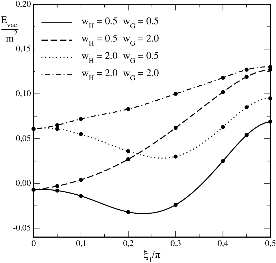
We find the VPE to be positive for most values of the variational parameters, so that it does not contribute to binding. For narrow string configurations (small width parameters) negative results are indeed obtained. For them to overcome the classical energy ($\mu_{H}=m_{H}/m$ is the scaled Higgs mass)

and bind the string, large Yukawa coupling constants are needed which eventually brings the Landau ghost problem into the game. Thus such bound configurations should not be considered [9].

In particular wide strings (which are not affected by the Landau ghost problem) generate many fermion bound states. Their energy eigenvalues are of the same order in the semi–classical $\hbar$ expansion as the VPE. Hence the inclusion of these levels ultimately enforces the consideration of the VPE.

Populating these levels can thus produce a configuration with finite charge (per unit length) $Q$ whose total energy per unit length is less than $Qm$. Subtracting the latter gives the total binding energy (also per unit length)

where $\epsilon_{i}$ and $p^{F}_{i}(Q)$ are the energy eigenvalues of $H$ with $0\leq\epsilon_{i}<m$ and the corresponding Fermi momenta, respectively. For a prescribed charge $Q$ we find an upper bound of $E_{\rm tot}(Q)$ by scanning several hundred configurations that are parameterized by different values of $w_{H}$, $w_{G}$ and $\xi_{1}$.

Numerical results for the upper bound of $E_{\rm tot}(Q)$ are shown in figure 2.

For $f>f_{c}\approx 1.7$ the total binding energy turns indeed negative and we have succeeded in constructing a bound string configuration [11]. This critical value is only about twice as big as the Yukawa coupling of the top quark in the standard model.

We have developed a procedure to compute the VPE of cosmic strings with spectral methods [12]. We have verified this procedure numerically by reproducing the required invariances even though the individual entries of the calculation are not invariant by themselves. We have found that the VPE does not bind classically unstable string configurations. When charging the string by populating fermion bound states, a stable configuration is obtained for fermions only about twice as heavy as the top quark. This must be considered a novel solution in a standard model like theory.