跳到论文正文
W Papers独立论文阅读器 arXiv:1609.08383 论文正文 计算阅读时间 · 0%
引用这篇论文根据当前论文元数据生成,正式投稿前建议核对。


License: arXiv.org perpetual non-exclusive license
arXiv:1609.08383v1 [quant-ph] 27 Sep 2016

Quantization of the 1-D harmonic oscillator with variable mass using the operators v^\hat{v} and p^\hat{p}

Gustavo V. López Note: gulopez@cencar.udg.mx    Eric M. Reynaga Affiliation: Departamento de Física, Universidad de Guadalajara, Affiliation: Blvd. Marcelino García Barragan y Calzada Olímpica, Affiliation: Ê44200 Guadalajara, Jalisco, Mexico
Abstract

For the 1-D harmonic oscillator with position depending variable mass, a Hamiltonian and constant of motion are given through a consistent approach. Then, the quantization of this system is carried out using the operator p^\hat{p}, for the Hamiltonian, and the operator v^\hat{v} for the constant of motion. We find that the result of both quantizations brings about different quantum dynamics.

1 Introduction

Mass variable systems have been important since the beginning of the Classical Mechanics [1-5], and now they are becoming even important in Quantum Mechanics [6-9]. These type of systems are not invariant under Galileo (non relativistic) or Lorentz (relativistic) transformations [10]. However, Newton’s equation of motion can be still be used to study these non relativistic systems [11] as a good approximation of their dynamics. Taking this point of view, a consistent approach for 1-D conservative systems with position depending mass [12] has been already made, where an effective potential depending of the variation of mass appears. This effective potential is missing in other approaches [15,16,17] where quantization of these systems is also studied. We consider that this effective potential must be included in any attempt to get a Lagrangian or Hamiltonian for these type of systems, and, of course, it must have a great deal of importance when one is dealing with the quantization of these systems. In this paper, we will use the effective potential approach to study the quantization of the harmonic oscillator with position depending mass. In addition, we make the comparison of the energy labels resulting from the quantization of the Hamiltonian ( using the x^\hat{x} and p^=−iℏ∂/∂x\hat{p}=-i\hbar\partial/\partial x operators), and the quantization of the constant of motion ( using the x^\hat{x} and v^=−i(ℏ/m)∂/∂x\hat{v}=-i(\hbar/m)\partial/\partial x operators).
Ê

2 Constant of motion and Hamiltonian

There is an expressions found in [12] for the constant of motion and Hamiltonian of a conservative system with position depending mass,

K⁡(x,v)=m2​(x)​v22​m0−1m0​∫x0xm⁡(s)​F​(s)​𝑑sK(x,v)=\frac{m^{2}(x)v^{2}}{2m_{0}}-\frac{1}{m_{0}}\int_{x_{0}}^{x}m(s)F(s)~ds (1a)
and
H⁡(x,p)=m0​p22​m2​(x)−1m0​∫x0xm⁡(s)​F​(s)​𝑑s,H(x,p)=\frac{m_{0}p^{2}}{2m^{2}(x)}-\frac{1}{m_{0}}\int_{x_{0}}^{x}m(s)F(s)~ds, (1b)

where m0=m⁡(x0)m_{0}=m(x_{0}), and x0x_{0} are the mass and the position of the particle at the initial time t0t_{0}, and F⁡(x)F(x) is the external conservative force. Applying these expression for the harmonic oscillator, where the force is given by F⁡(x)=−k​xF(x)=-kx (with kk being a constant), the above expressions are written as

K⁡(x,v)=m2​(x)​v22​m0+km0​∫x0xs​m​(s)​𝑑sK(x,v)=\frac{m^{2}(x)v^{2}}{2m_{0}}+\frac{k}{m_{0}}\int_{x_{0}}^{x}sm(s)~ds (2a)
and
H⁡(x,p)=m0​p22​m2​(x)+km0​∫x0xs​m​(s)​𝑑s,H(x,p)=\frac{m_{0}p^{2}}{2m^{2}(x)}+\frac{k}{m_{0}}\int_{x_{0}}^{x}sm(s)~ds, (2b)

To proceed with the analysis, one needs a model for m⁡(x)m(x). Let us assume that

m⁡(x)=m0+m1​x,m(x)=m_{0}+m_{1}x, (3)

where m1=d​m​(x)/d​xm_{1}=dm(x)/dx is the rate of increasing or decreasing the mass of the system. With this model, the constant of motion and Hamiltonian are (x0=0x_{0}=0)

K⁡(x,v)=(m0+m1​x)22​m0​v2+12​m0​ω2​x2+m1​ω23​x3K(x,v)=\frac{(m_{0}+m_{1}x)^{2}}{2m_{0}}v^{2}+\frac{1}{2}m_{0}\omega^{2}x^{2}+\frac{m_{1}\omega^{2}}{3}x^{3} (4a)
and
H⁡(x,p)=m0​p22​(m0+m1​x)2+12​m0​ω2​x2+m1​ω23​x3,H(x,p)=\frac{m_{0}p^{2}}{2(m_{0}+m_{1}x)^{2}}+\frac{1}{2}m_{0}\omega^{2}x^{2}+\frac{m_{1}\omega^{2}}{3}x^{3}, (4b)

where we have defined ω=k/m0\omega=\sqrt{k/m_{0}}. Assuming m1​x/m0≪1m_{1}x/m_{0}\ll 1 and using up to second order in Taylor expansion in the Hamiltonian, these expression are

K⁡(x,v)=12​m0​v2+12​m0​ω2​x2+m1​x​v2+m122​m0​x2​v2+m1​ω23​x3K(x,v)=\frac{1}{2}m_{0}v^{2}+\frac{1}{2}m_{0}\omega^{2}x^{2}+m_{1}xv^{2}+\frac{m_{1}^{2}}{2m_{0}}x^{2}v^{2}+\frac{m_{1}\omega^{2}}{3}x^{3} (5a)
and
H⁡(x,p)=p22​m0+12​m0​ω2​x2+(−m1​xm0+3​m12​x22​m02)​p2m0+m1​ω23​x3,H(x,p)=\frac{p^{2}}{2m_{0}}+\frac{1}{2}m_{0}\omega^{2}x^{2}+\biggl(-\frac{m_{1}x}{m_{0}}+\frac{3m_{1}^{2}x^{2}}{2m_{0}^{2}}\biggr)\frac{p^{2}}{m_{0}}+\frac{m_{1}\omega^{2}}{3}x^{3}, (5b)

that is, the constant of motion and Hamiltonian are of the form

K=K0+WK,K=K_{0}+W_{K}, (6)

and

H=H0+WH,H=H_{0}+W_{H}, (7)

where K0K_{0}, WKW_{K}, H0H_{0}, and WHW_{H} are defined as

K0=12​m0​v2+12​m0​ω2​x2,K_{0}=\frac{1}{2}m_{0}v^{2}+\frac{1}{2}m_{0}\omega^{2}x^{2}, (8a)
WK=m1​x​v2+m122​m0​x2​v2+m1​ω23​x3W_{K}=m_{1}xv^{2}+\frac{m_{1}^{2}}{2m_{0}}x^{2}v^{2}+\frac{m_{1}\omega^{2}}{3}x^{3} (8b)
,
H0=p22​m0+12​m0​ω2​x2,H_{0}=\frac{p^{2}}{2m_{0}}+\frac{1}{2}m_{0}\omega^{2}x^{2}, (9a)
and
WH=(−m1​xm0+3​m12​x22​m02)​p2m0+m1​ω23​x3.W_{H}=\biggl(-\frac{m_{1}x}{m_{0}}+\frac{3m_{1}^{2}x^{2}}{2m_{0}^{2}}\biggr)\frac{p^{2}}{m_{0}}+\frac{m_{1}\omega^{2}}{3}x^{3}. (9b)

3 Quantization

To see whether or not the quantum dynamics described by the relations (6) and (7) are different, it is enough to consider WKW_{K} and WHW_{H} as perturbation of K0K_{0} and H0H_{0} respectively. The quantization with the Hamiltonian is carried out through the usual association of an Hermitian operator H^​(x^,p^){\widehat{H}}(\hat{x},\hat{p}) [13], being the Hermitian operator p^\hat{p} defined as p^=−iℏ∂/∂x\hat{p}=-i\hbar\partial/\partial x, and solving the Schrödinger’s equation

i​ℏ​∂Ê​|Ψ⟩∂t=H^​(x^,p^)​|Ψ⟩.i\hbar\frac{\partial Ê|\Psi\rangle}{\partial t}={\widehat{H}}(\hat{x},\hat{p})|\Psi\rangle. (10)

The quantization with the constant of motion is also carried out through the association of an Hermitian operator K^​(x^,v^){\widehat{K}}(\hat{x},\hat{v}), being the Hermitian operator v^\hat{v} defined as v^=−i(ℏ/m0)∂/∂x\hat{v}=-i(\hbar/m_{0})\partial/\partial x, and solving the Schrödinger-like equation

i​ℏ​∂|Ψ⟩∂t=K^​(x^,v^)​|Ψ⟩.i\hbar\frac{\partial|\Psi\rangle}{\partial t}={\widehat{K}}(\hat{x},\hat{v})|\Psi\rangle. (11)

Because of the expressions (5a) and (5b), the equations (10) and (11) corresponds to autonomous systems, the proposition

|Ψ⟩=e−iEt/ℏ|Φ⟩|\Psi\rangle=e^{-iEt/\hbar}|\Phi\rangle (12)

reduces the solutions to solve the eigenvalue problems

H^​|Φ⟩H=EH​|Φ⟩H,{\widehat{H}}|\Phi\rangle_{H}=E_{H}|\Phi\rangle_{H}, (13)

and

K^​|Φ⟩K=EK​|Φ⟩K.{\widehat{K}}|\Phi\rangle_{K}=E_{K}|\Phi\rangle_{K}. (14)

Since WHW_{H} and WKW_{K} are considered as perturbations of the harmonic oscillator with constant mass , it is enough to know the eigenvalues up to second order in perturbation theory to see whether or not there is a difference on the quantum dynamics. From the perturbation theory, it is well known [13] that up to second order on perturbation theory, the eigenvalues are given as

Eξ,n=Eξ,n(0)+Eξ,n(1)+Eξ,n(2),ξ=H,K,E_{\xi,n}=E_{\xi,n}^{(0)}+E_{\xi,n}^{(1)}+E_{\xi,n}^{(2)},\quad\quad\xi=H,K, (15)

with Eξ,n(0)E_{\xi,n}^{(0)} being the eigenvalues associated to H0H_{0} or K0K_{0},

En(0)=EH,n(0)=EK,n(0)=ℏ​ω​(n+1/2).n∈𝒵+,E_{n}^{(0)}=E_{H,n}^{(0)}=E_{K,n}^{(0)}=\hbar\omega(n+1/2).\quad\quad n\in{\cal Z^{+}}, (16)

and Eξ,n(1)E_{\xi,n}^{(1)} and Eξ,n(2)E_{\xi,n}^{(2)} are given by

Eξ,n(1)=⟨n|W^ξ|n⟩E_{\xi,n}^{(1)}=\langle n|\widehat{W}_{\xi}|n\rangle (17)

and

Eξ,n(2)=∑m≠n|⟨m|W^ξ|n⟩|2En(0)−Em(0).E_{\xi,n}^{(2)}=\sum_{m\not=n}\frac{\displaystyle|\langle m|\widehat{W}_{\xi}|n\rangle|^{2}}{E_{n}^{(0)}-E_{m}^{(0)}}. (18)

The eigenstates {|n⟩}\{|n\rangle\} are the eigenstates of H0H_{0} or K0K_{0} which represents the functions

Φn(x)=⟨x|n⟩=cne−α2x2/2Hn(αx),cn=απ​2n​n!,\Phi_{n}(x)=\langle x|n\rangle=c_{n}e^{-\alpha^{2}x^{2}/2}H_{n}(\alpha x),\quad\quad c_{n}=\sqrt{\frac{\alpha}{\sqrt{\pi}~2^{n}n!}}, (19)

being HnH_{n} represents the Hermit polynomials, and the constant α\alpha is given by α=m​ω/ℏ\alpha=\sqrt{m\omega/\hbar}.

3.1 Eigenvalues of EH,nE_{H,n}.

As we can see from (5b), one requires to assign Hermitian operators to the functions x​p2xp^{2}, x2​p2x^{2}p^{2} and x3x^{3}. This can be obtained by using Weyl quantization method [14], or identifying the powers of polynomial (x+p)l(x+p)^{l} with the powers of operator polynomial (x^+p^)l(\hat{x}+\hat{p})^{l} for l=2,4l=2,4. Doing either of these approaches, and using the commutation relation [x^,p^]=i​ℏ​I[\hat{x},\hat{p}]=i\hbar I (being I the identity operator), one gets

x​p2^=x^​p^2−i​ℏ​p^,\widehat{xp^{2}}=\hat{x}\hat{p}^{2}-i\hbar\hat{p}, (20a)
x2​p2^=x^2​p^2−i​2​ℏ​x^​p^−ℏ22​I,\widehat{x^{2}p^{2}}=\hat{x}^{2}\hat{p}^{2}-i2\hbar\hat{x}\hat{p}-\frac{\hbar^{2}}{2}I, (20b)
and
x3^=x^3.\widehat{x^{3}}=\hat{x}^{3}. (20c)

In this way, the associated Hermitian operator to the function WHW_{H} is

W^H=−m1m02(x^p^2−iℏp^)+3​m122​m03(x^2p^2−i2ℏx^p^−ℏ22)+m1​ω23x^3.\widehat{W}_{H}=-\frac{m_{1}}{m_{0}^{2}}\bigl(\hat{x}\hat{p}^{2}-i\hbar\hat{p}\bigr)+\frac{3m_{1}^{2}}{2m_{0}^{3}}\bigr(\hat{x}^{2}\hat{p}^{2}-i2\hbar\hat{x}\hat{p}-\frac{\hbar^{2}}{2}\bigr)+\frac{m_{1}\omega^{2}}{3}\hat{x}^{3}. (21)

for convenience during evaluation of the matrix elements of the perturbation terms, one uses the ascent (a†a^{\dagger}) and descent (aa) operators instead of x^\hat{x} and p^\hat{p},

x^=ℏ2​m0​ω​(a+a†)andp^=−i​m0​ℏ​ω2​(a−a†),\hat{x}=\sqrt{\frac{\hbar}{2m_{0}\omega}}~(a+a^{\dagger})\quad\quad\hbox{and}\quad\hat{p}=-i\sqrt{\frac{m_{0}\hbar\omega}{2}}~(a-a^{\dagger}), (22)

where one has the following properties

a|n⟩=n|n−1⟩,a†|n⟩=n+1|n+1⟩,and[a,a†]=1.a|n\rangle=\sqrt{n}|n-1\rangle,\quad a^{\dagger}|n\rangle=\sqrt{n+1}|n+1\rangle,\quad\hbox{and}\quad[a,a^{\dagger}]=1. (23)

Thus, one obtains W^H\widehat{W}_{H} in terms of aa and a†a^{\dagger} as

W^H\displaystyle\widehat{W}_{H} =\displaystyle= −m1​ℏ​ω2​m0​ℏ2​m0​ω​(a3−a2​a†−a​a†​a+a​(a†)2+a†​a2−a†​a​a†−(a†)2​a+a3)−m1​ℏm02​m0​ℏ​ω2​(a−a+)\displaystyle-\frac{\displaystyle m_{1}\hbar\omega}{\displaystyle 2m_{0}}\sqrt{\displaystyle\frac{\hbar}{\displaystyle 2m_{0}\omega}}\biggl(a^{3}-a^{2}a^{\dagger}-aa^{\dagger}a+a(a^{\dagger})^{2}+a^{\dagger}a^{2}-a^{\dagger}aa^{\dagger}-(a^{\dagger})^{2}a+a^{3}\biggr)-\frac{m_{1}\hbar}{m_{0}^{2}}\sqrt{\frac{m_{0}\hbar\omega}{2}}~\bigl(a-a^{+}\bigr) (24)
−3​m12​ℏ28​m03​(a4−a2​a†​a−a2​(a†)2+a†​a3−a†​a​a†​a−a†​a2​a†+a†​a​(a†)2+a​a†​a2−a3​a†−(a†)2​a​a†CLOSE\displaystyle-\frac{\displaystyle 3m_{1}^{2}\hbar^{2}}{8m_{0}^{3}}\biggl(a^{4}-a^{2}a^{\dagger}a-a^{2}(a^{\dagger})^{2}+a^{\dagger}a^{3}-a^{\dagger}aa^{\dagger}a-a^{\dagger}a^{2}a^{\dagger}+a^{\dagger}a(a^{\dagger})^{2}+aa^{\dagger}a^{2}-a^{3}a^{\dagger}-(a^{\dagger})^{2}aa^{\dagger}
OPEN−a2​a†​a−a​a†​a​a†+a​(a†)3+(a†)2​a2−(a†)3​a+(a†)4)\displaystyle\quad\quad\quad\quad\quad-a^{2}a^{\dagger}a-aa^{\dagger}aa^{\dagger}+a(a^{\dagger})^{3}+(a^{\dagger})^{2}a^{2}-(a^{\dagger})^{3}a+(a^{\dagger})^{4}\biggr)
−3​m12​ℏ22​m03​(a2−a​a†+a†​a−(a†)2+12)\displaystyle-\frac{\displaystyle 3m_{1}^{2}\hbar^{2}}{2m_{0}^{3}}\biggl(a^{2}-aa^{\dagger}+a^{\dagger}a-(a^{\dagger})^{2}+\frac{1}{2}\biggr)
+m1​ω23​(ℏ2​m0​ω)3/2​(a3+a​a†​a+a2​a†+a​(a†)2+a†​a2+(a†)2​a+a†​a​a†+(a†)3)\displaystyle+\frac{\displaystyle m_{1}\omega^{2}}{\displaystyle 3}\left(\frac{\displaystyle\hbar}{\displaystyle 2m_{0}\omega}\right)^{3/2}\biggl(a^{3}+aa^{\dagger}a+a^{2}a^{\dagger}+a(a^{\dagger})^{2}+a^{\dagger}a^{2}+(a^{\dagger})^{2}a+a^{\dagger}aa^{\dagger}+(a^{\dagger})^{3}\biggr)

Therefore, using (12), (24) in (17) and (18), it follows that

EH,n(1)=σ⁡{2​n2+2​n−14+12}E_{H,n}^{(1)}=\sigma\left\{\frac{2n^{2}+2n-1}{4}+\frac{1}{2}\right\} (25a)
and
EH,n(2)=−1ℏ​ω​{(η−m1​β)2​(3​n2+3​n+2)+(3​η−m1​β)2​(3​n3+3​n+1)+(σ4)2​(4​n3+6​n2+14​n+6)},E_{H,n}^{(2)}=-\frac{1}{\hbar\omega}\left\{(\eta-m_{1}\beta)^{2}(3n^{2}+3n+2)+(3\eta-m_{1}\beta)^{2}(3n^{3}+3n+1)+\left(\frac{\sigma}{4}\right)^{2}(4n^{3}+6n^{2}+14n+6)\right\}, (25b)

where the constants σ\sigma, β\beta, and η\eta have been defined as

σ=3​m12​ℏ22​m03,β=ℏ2​m0ℏ​ω2​m0,andη=m1​ω23(ℏ2​m0​ω)3/2.\sigma=\frac{3m_{1}^{2}\hbar^{2}}{2m_{0}^{3}},\quad\quad\beta=\frac{\hbar}{2m_{0}}\sqrt{\frac{\hbar\omega}{2m_{0}}},\quad\hbox{and}\quad\eta=\frac{m_{1}\omega^{2}}{3}\left(\frac{\hbar}{2m_{0}\omega}\right)^{3/2}. (26)

Thus, up to second order in perturbation theory, the energy of the system of the nth-state is

EH,n\displaystyle E_{H,n} =\displaystyle= ℏ​ω​(n+1/2)+σ⁡{2​n2+2​n−14+12}\displaystyle\hbar\omega(n+1/2)+\sigma\left\{\frac{2n^{2}+2n-1}{4}+\frac{1}{2}\right\}
−1ℏ​ω​{(η−m1​β)2​(3​n2+3​n+2)+(3​η−m1​β)2​(3​n3+3​n+1)+(σ4)2​(4​n3+6​n2+14​n+6)}.\displaystyle-\frac{1}{\hbar\omega}\left\{(\eta-m_{1}\beta)^{2}(3n^{2}+3n+2)+(3\eta-m_{1}\beta)^{2}(3n^{3}+3n+1)+\left(\frac{\sigma}{4}\right)^{2}(4n^{3}+6n^{2}+14n+6)\right\}.

3.2 Eigenvalues of EK,nE_{K,n}

As we can see from expression (5a), and from the previous calculation we have made, one needs to assign Hermitian operators to the functions x​v2xv^{2}, x2​v2​4x^{2}v^{2}4 and x3x^{3}. In this case, one has that

v^=−i​ℏm0​∂∂x,and[x^,v^]=i​ℏm0​I.\hat{v}=-i\frac{\hbar}{m_{0}}\frac{\partial}{\partial x},\quad\quad\hbox{and}\quad[\hat{x},\hat{v}]=i\frac{\hbar}{m_{0}}I. (28)

Using the same method we used previously and the commutation relation (28), one has the following Hermitian operator for WKW_{K}

W^K=m1​(x^​v^2−i​ℏm0​v^)+m122​m0​(x^2​v^2−i​2​ℏm0​x^​v^−ℏ22​m02)+m1​ω23​m0​x^3.\widehat{W}_{K}=m_{1}\biggl(\hat{x}\hat{v}^{2}-i\frac{\hbar}{m_{0}}\hat{v}\biggr)+\frac{m_{1}^{2}}{2m_{0}}\biggl(\hat{x}^{2}\hat{v}^{2}-i\frac{2\hbar}{m_{0}}\hat{x}\hat{v}-\frac{\hbar^{2}}{2m_{0}^{2}}\biggr)+\frac{m_{1}\omega^{2}}{3m_{0}}\hat{x}^{3}. (29)

Now, instead of the operators x^\hat{x} and v^\hat{v} , one changes to the ascend (a†a^{\dagger}) and descend (aa) operators through the relations

x^=ℏ2​m0​ω​(a+a†),andv^=−i​ℏ​ω2​m0​(a−a†),\hat{x}=\sqrt{\frac{\hbar}{2m_{0}\omega}}~(a+a^{\dagger}),\quad\quad\hbox{and}\quad\hat{v}=-i\sqrt{\frac{\hbar\omega}{2m_{0}}}~(a-a^{\dagger}), (30)

where aa and a†a^{\dagger} have the same properties written in (12). Proceeding similarly as what we did previously, one gets the following expression for W^K\widehat{W}_{K}

W^K\displaystyle\widehat{W}_{K} =\displaystyle= −ℏ2​m1m0​ℏ​ω2​m0​(a^3−a^2​a^+−a^​a^+​a^+a^​a^+2+a^+​a^2−a^+​a^​a^+−a^+2​a^+a^+3)−2​m1​β​(a^−a^+)\displaystyle-\frac{\hbar}{2}\frac{m_{1}}{m_{0}}\sqrt{\frac{\hbar\omega}{2m_{0}}}\biggl(\hat{a}^{3}-\hat{a}^{2}\hat{a}^{+}-\hat{a}\hat{a}^{+}\hat{a}+\hat{a}\hat{a}^{+2}+\hat{a}^{+}\hat{a}^{2}-\hat{a}^{+}\hat{a}\hat{a}^{+}-\hat{a}^{+2}\hat{a}+\hat{a}^{+3}\biggr)-2m_{1}\beta(\hat{a}-\hat{a}^{+})
−α12{a^4−a^2a^+a^−a^2a^+2+a^+a^3−a^+a^a^+a^−a^+a^2a^++a^+a^a^+2+a^a^+a^2−a^a^+2a^−a3a†\displaystyle-\frac{\alpha}{12}\biggl\{\hat{a}^{4}-\hat{a}^{2}\hat{a}^{+}\hat{a}-\hat{a}^{2}\hat{a}^{+2}+\hat{a}^{+}\hat{a}^{3}-\hat{a}^{+}\hat{a}\hat{a}^{+}\hat{a}-\hat{a}^{+}\hat{a}^{2}\hat{a}^{+}+\hat{a}^{+}\hat{a}\hat{a}^{+2}+\hat{a}\hat{a}^{+}\hat{a}^{2}-\hat{a}\hat{a}^{+2}\hat{a}-a^{3}a^{\dagger}
−a^a^+a^a^++a^a^+3+a^+2a^2−a^+3a^−a^+2a^a^++a^+4}\displaystyle\quad\quad\quad\quad\quad-\hat{a}\hat{a}^{+}\hat{a}\hat{a}^{+}+\hat{a}\hat{a}^{+3}+\hat{a}^{+2}\hat{a}^{2}-\hat{a}^{+3}\hat{a}-\hat{a}^{+2}\hat{a}\hat{a}^{+}+\hat{a}^{+4}\biggr\}
Ê\displaystyle Ê
−12​m12​ℏ2m03​(a^2−a^​a^+−a^+​a^+a^+2+12)\displaystyle-\frac{1}{2}\frac{m_{1}^{2}\hbar^{2}}{m_{0}^{3}}\biggl(\hat{a}^{2}-\hat{a}\hat{a}^{+}-\hat{a}^{+}\hat{a}+\hat{a}^{+2}+\frac{1}{2}\biggr)
Ê\displaystyle Ê (31)
+ω2​m13​(ℏ2​m0​ω)3/2​(a^3+a^​a^+​a^+a^2​a^++a^​a^+2+a^+​a^2+a^+2​a^+a^+​a^​a^++a^+3)\displaystyle+\frac{\omega^{2}m_{1}}{3}\left(\frac{\hbar}{2m_{0}\omega}\right)^{3/2}\biggl(\hat{a}^{3}+\hat{a}\hat{a}^{+}\hat{a}+\hat{a}^{2}\hat{a}^{+}+\hat{a}\hat{a}^{+2}+\hat{a}^{+}\hat{a}^{2}+\hat{a}^{+2}\hat{a}+\hat{a}^{+}\hat{a}\hat{a}^{+}+\hat{a}^{+3}\biggr)

From this expression, we get

EK,n(1)=σ3​(2​n2+2​n−14+12)E_{K,n}^{(1)}=\frac{\sigma}{3}\biggl(\frac{2n^{2}+2n-1}{4}+\frac{1}{2}\biggr) (32a)
and
EK,n(2)=−1ℏ​ω​{(η−m1​β)2​(3​n2+3​n+2)+(3​η+m1​β)2​(3​n2+3​n+1)+(σ12)2​(4​n3+6​n2+14​n+6)}.E_{K,n}^{(2)}=-\frac{1}{\hbar\omega}\left\{(\eta-m_{1}\beta)^{2}(3n^{2}+3n+2)+(3\eta+m_{1}\beta)^{2}(3n^{2}+3n+1)+\left(\frac{\sigma}{12}\right)^{2}(4n^{3}+6n^{2}+14n+6)\right\}. (32b)

So, the energy associated to the quantization of the constant of motion in the nth-state is

EK,n\displaystyle E_{K,n} =\displaystyle= ℏ​ω​(n+1/2)+σ3​(2​n2+2​n−14+12)\displaystyle\hbar\omega(n+1/2)+\frac{\sigma}{3}\biggl(\frac{2n^{2}+2n-1}{4}+\frac{1}{2}\biggr)
−1ℏ​ω​{(η−m1​β)2​(3​n2+3​n+2)+(3​η+m1​β)2​(3​n2+3​n+1)+(σ12)2​(4​n3+6​n2+14​n+6)}.\displaystyle-\frac{1}{\hbar\omega}\left\{(\eta-m_{1}\beta)^{2}(3n^{2}+3n+2)+(3\eta+m_{1}\beta)^{2}(3n^{2}+3n+1)+\left(\frac{\sigma}{12}\right)^{2}(4n^{3}+6n^{2}+14n+6)\right\}.

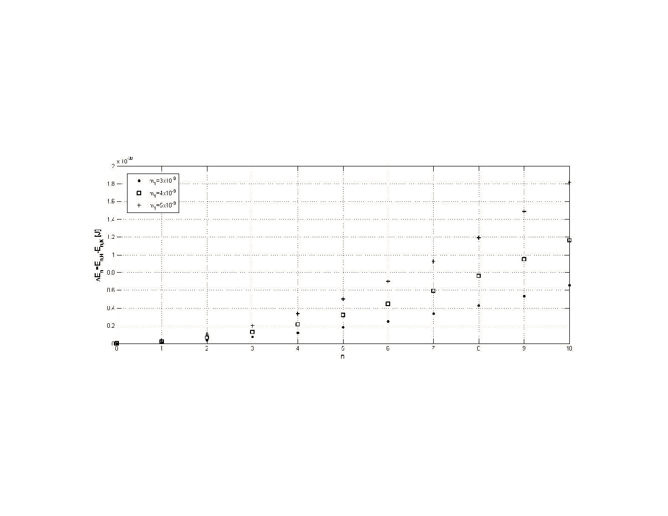
The difference in the energy levels for the two methods of quantization (Δ​En=EH,n−EK,n\Delta E_{n}=E_{H,n}-E_{K,n}) is

Δ​En=2​σ3​(14​(2​n2+2​n−1)+12)+4​m1​η​βℏ​ω​(6​n2+6​n+1)−σ218​ℏ​ω​(4​n3+6​n2+14​n+6).\Delta E_{n}=\frac{2\sigma}{3}\left(\frac{1}{4}(2n^{2}+2n-1)+\frac{1}{2}\right)+\frac{4m_{1}\eta\beta}{\hbar\omega}(6n^{2}+6n+1)-\frac{\sigma^{2}}{18\hbar\omega}(4n^{3}+6n^{2}+14n+6). (34)

this difference is plotted in the next figure for m0=10−17​K​gm_{0}=10^{-17}Kg, ω=10​G​H​z\omega=10~GHz, and for values of m1m_{1} (units of Kg/m) such that Eξ,n(1)+Eξ,n(2)E_{\xi,n}^{(1)}+E_{\xi,n}^{(2)} be lower than 1%1\% of En(0)E_{n}^{(0)}.

Refer to caption
Figure 1: Difference on energies for the two cases.

4 Conclusions

We have made the study of the quantization of 1-D harmonic oscillator with position depending mass. We used two methods of quantization, one due to the usual Hamiltonian approach, and the other one is proposed approach based on the quantization of a constant of motion of the system. On both approaches, the Shrödinger’s equation is used to see the quantum dynamics of the system. The position depending mass produces an additional term which is taken as a perturbation of the usual harmonic oscillator with constant mass. Using perturbation theory at second order, the energies associated to the Hamiltonian and constant of motion approaches was give, obtaining a difference in their values.This difference is not due to the fact that the resulting expression for K is exact , meanwhile for the Hamiltonian is an approximation to second order in Taylor expansion. Finally, it is our expectation that an experiment can be carried out to see whether or not the mass position approach and K-quantization approach can be verified experimentally.

References
Ê
1. H. Goldstein, Classical Mechanics, Addison-Wesley, (1950).

2. S.K. Bose, The rocket problem revisited, Am. J. Phys., 51, (1983), 463.

3. A. Sommerfeld, Lectures on Theoretical Physics, vol. I, Academic Press, (1964).

4. H. Gyden, Astronomische Nachrichtem, 109, (1884), 1.

5, I.V. Meshcherskii, Astronomische Nachrichtem, 132, (1893),93.

6. C. Tuiega, J. jasiski, T. Iwamoto, and V. Chikan, ACS Nano, 2, (2008), 1411.

7. H.A. Bethe, Phys. Rev. Lett., 56, (1936), 1305.

8. E.D. Comminss and P.A. Bucksbaum, Weak Interactions of Leptons and Quarks, Cambridge University Press, (1983).

9. O. Tokamobu, D. Kentare, N. Koichi, and T. Akitomo, Physica Status Solidi, B241, (2004), 2744.

10. G.V. López and E.M. Juárez, J. Mod. Phys., 4, (2013), 1638.

11. M. Spivak, Physics for Mathematisians, Mechanics I, Publish or Perish, Inc. (2010).

12. G.V. López and C. Martínez-Prieto, J. Mod. Phys., 5, (2014), 900.

13. A. Messiah, Quantum Mechanics, dover, (1999).

14. H. Weyl, Quantummechanick und Gruppentheorie, Z.T. Physics, 46, (1927),1.
Ê
15. S. Cruz y Cruz, Geometric Methdos in Physics, XXX Workshop 2011. Trends in Mathematics, (2011), 229.
Ê
16. M.S. Cunha and H.R. Christiansen, Comm. Theor. Phys.,60, (2013), 642.

17. S. Cruz y Cruz and O. Rosas-Ortiz, J. Phys. A: Math. Theor.,42, (2009), 185205.