Smoothings and Rational Double Point Adjacencies for Cusp Singularities
Abstract
A cusp singularity is a surface singularity whose minimal resolution is a cycle of smooth rational curves meeting transversely. Cusp singularities come in dual pairs. Looijenga proved in 1981 that if a cusp singularity is smoothable, the minimal resolution of the dual cusp is the anticanonical divisor of some smooth rational surface. In 1983, the second author and Miranda gave a criterion for smoothability of a cusp singularity, in terms of the existence of a K-trivial semistable model for the central fiber of such a smoothing. We study these “Type III degenerations” of rational surfaces with an anticanonical divisor—their deformations, birational geometry, and monodromy. Looijenga’s original paper also gave a description of the rational double point configurations to which a cusp singularity deforms, but only in the case where the resolution of the dual cusp has cycle length 5 or less. We generalize this classification to an arbitrary cusp singularity, giving an explicit construction of a semistable simultaneous resolution of such an adjacency. The main tools of the proof are (1) formulas for the monodromy of a Type III degeneration, (2) a construction via surgeries on integral-affine surfaces of a degeneration with prescribed monodromy, (3) surjectivity of the period map for Type III central fibers, and (4) a theorem of Shepherd-Barron producing a simultaneous contraction to the adjacency.
Introduction
Let be the germ of an isolated singularity. Some basic questions that one can ask about the deformation theory of are: Is smoothable? If so, how can we describe the smoothing components of ? What are the singularities adjacent to ? In particular, for a surface singularity, what are the rational double points adjacent to ? In case is itself a rational double point, the answers to these questions are well-known. In this case, is smoothable and there is a unique smoothing component, as it is a hypersurface singularity, and the adjacent rational double points correspond to subgraphs of the Dynkin diagram corresponding to .
The next level of complexity for a normal surface singularity is the case where is a minimally elliptic singularity in Laufer’s terminology, i.e. a Gorenstein elliptic singularity, and here the simplest case is when the fundamental cycle of is reduced. In this case, is either a simple elliptic, cusp, or triangle singularity. These three types admit a resolution whose exceptional fiber is a smooth elliptic curve, a cycle of smooth rational curves, or either cuspidal, two smooth rational curves meeting at a tacnode, or three smooth rational curves meeting at a point, respectively.
The deformation theory of simple elliptic and triangle singularities is by now well understood, by work of Pinkham and Looijenga [32], [33], [25], [26]. The crucial point here is that the singularities in question have a -action. Thus questions about smoothings and adjacent singularities can be related to global questions about the existence of certain compact algebraic surfaces with configurations of curves on them: (generalized) del Pezzo surfaces with a smooth section of the anticanonical divisor in the case of simple elliptic singularities, surfaces with so-called configurations in the case of triangle singularities. For example, in case is simple elliptic, let be the minimal resolution of and set . Then we may realize the germ on an elliptically ruled surface with zero section and infinity section satisfying . We preserve the divisor on the nearby fibers of a negative weight deformation of to get pairs , where is a normal projective surface such that .
It follows that nontrivial negative weight deformations of correspond to generalized del Pezzo surfaces , hence whenever is smoothable (the converse also holds). Furthermore, the adjacent configurations of rational double points to are those that appear on such an . These in turn can be described by the configurations of curves, all of whose components are isomorphic to and of self-intersection , which appear as the exceptional curves on a minimal resolution . For small, is a complete intersection singularity () or a Pfaffian singularity (). In this case, there is an associated root system given by taking the vectors of square in . (By the usual algebraic geometry conventions, all root systems in this paper will be negative definite.) Then the possible Dynkin diagrams of configurations of rational double points on some are given by root systems contained in satisfying a mild extra condition coming from the period map, which can in turn be described via embeddings into the extended Dynkin diagram of . For large, however, there can be several smoothing components of and need not be a root lattice. Nonetheless, the possible adjacent rational double point configurations can still be described lattice-theoretically.
For the case of cusp singularities, Looijenga gave a beautiful description of the possible adjacencies in his breakthrough paper [27], but only in the case of multiplicity at most . In this case, the cusp singularity is either a complete intersection or Pfaffian, hence automatically smoothable and there is a unique smoothing component. As in the case of simple elliptic singularities of multiplicity at most , there is again a diagram which determines the possible adjacent singularities, and it is the intersection graph for the root basis of a generalized root system of hyperbolic type.
As above, a key ingredient in Looijenga’s analysis is the existence of a complete surface containing the cusp on which one globalizes deformations. But one must leave the world of algebraic geometry to produce such a surface. The Inoue surface associated to a cusp is a compact complex surface of type VII0 such that , where an analytic neighborhood of is a minimal resolution of the cusp , and by definition an analytic neighborhood of is a minimal resolution of the dual cusp to . (For notational reasons, it is more convenient to denote by the minimal resolution of the cusp we are interested in deforming and by the minimal resolution of its dual.) Here is a cycle of smooth rational curves, or an irreducible nodal curve if , and similarly for . By convention, , where the integer is taken mod , and otherwise. The type or self-intersection sequence of is the sequence mod cyclic permutations and order-reversing permutations. There is a somewhat complicated recipe for obtaining , together with its self-intersection sequence, from .
Looijenga showed that, if is the compact singular analytic surface obtained by contracting the curves and , then the deformation functor of is naturally isomorphic to . Thus, the deformations of , viewed as deformations of for which the deformation of is trivial, can be identified with deformations of the pair keeping constant, where is the compact singular analytic surface obtained by contracting . A smoothing of then yields a pair , where is a smooth rational surface and is a cycle of rational curves of the same type as . Briefly, we say that sits on a rational surface (we identify with ). Hence a smoothing component of determines a deformation type of anticanonical pairs , i.e. pairs consisting of a smooth rational surface and a section which is a cycle of rational curves of the same type as the minimal resolution of the dual cusp to . We define a smoothing component of to be of type in this case. In particular, the existence of such a pair is a necessary condition for the cusp to be smoothable. In [27], Looijenga conjectured that it is also a sufficient condition:
Conjecture 0.1 (Looijenga’s conjecture).
The cusp is smoothable if and only if the minimal resolution of the dual cusp sits on a rational surface.
Motivated by the corresponding picture for degenerations of surfaces, the second author and R. Miranda showed in [10] that Looijenga’s conjecture was equivalent to the existence of a certain semistable model for the smoothing, whose description we recall in Section 2. The main idea is to show that the semistable fiber deforms in a smooth one parameter family . Here is the Inoue surface with the cycles and , and the , , are rational surfaces meeting along the cycle . A theorem of Shepherd-Barron [34] shows that the divisor is exceptional in , although we might also have to contract some rational curves in the general fibers. (The theorem of Shepherd-Barron is stated in the context of degenerations of surfaces, but the proof applies in this setting as well.) The result is a singular complex threefold and a flat morphism such that the fiber over is the singular Inoue surface and the general fiber is a rational surface, possibly with rational double points. In particular, is smoothable. However, the complexity of constructing the possible semistable singular fibers seemed, in the words of [10], “rather daunting.”
Looijenga’s conjecture went unproven until quite recently. The first proof, due to Gross-Hacking-Keel [14], is based on ideas from the Gross-Siebert program [15] for proving mirror symmetry. The second proof, due to the first author [5], uses ideas from symplectic geometry to construct the semistable models that are required in the approach of [10]. The two proofs can be viewed, respectively, as part of the “algebraic” and the “symplectic” aspects of mirror symmetry for the anticanonical pair . While we have no proven claims regarding mirror symmetry, it serves as an underlying motivation for some of the constructions in this paper.
Mirror symmetry is, very roughly, a prediction originating in physics that Calabi-Yau varieties come in mirror pairs and on which algebraic and symplectic data are interchanged. Kontsevich [20] formalized these physical ideas in homological mirror symmetry—that the derived category of coherent sheaves on is equivalent to the Fukaya category of . The Strominger-Yau-Zaslow program [36] sought to derive a more geometric origin of mirror symmetry—that and have dual special Lagrangian torus fibrations over a common base .
Hitchin [17] observed that the base carries two natural integral-affine structures. These structures are interchanged by mirror symmetry. The Gross-Siebert program built on this observation, providing a new interpretation of these integral-affine structures on in terms of tropical geometry. Instead of just a Calabi-Yau variety , one should consider its “large complex structure limit”—a maximally unipotent degeneration of over a disc. Then one of the affine structures on is identified via the tropical geometry with the dual complex of the central fiber. This affine structure ought to agree with the affine structure on coming from the symplectic geometry of the Lagrangian torus fibration .
It is possible to understand the results of this paper within such a framework. Observe that a smoothing of is a degeneration of the open Calabi-Yau variety . This degeneration is the large complex structure limit. One expects then that the dual complex of the semistable resolution of the central fiber has two natural integral-affine structures. In Section 2.2 we describe one of these structures, which is the other structure than the one considered by Gross-Hacking-Keel. Our affine structure is identified with the base of a Lagrangian torus fibration of the mirror of over .
While [14] builds a smoothing of the cusp by a “polytope” construction from their integral-affine structure on , we follow [5] to build a semistable resolution of a smoothing by a “fan” construction from the other structure. One advantage of the approach of [14] is the construction of canonical theta functions on the deformation, analogous to theta functions on degenerations of abelian varieties. Furthermore, our approach only produces a one-parameter smoothing as opposed to a versal deformation of the cusp. However, the construction here and in [5] has many other advantages: the geometry of the degeneration, central fiber, and significantly, the semistable resolution, are much more explicit. One can algorithmically build the central fiber of the resolution of a smoothing of the cusp. Our methods yield a strengthening of Looijenga’s conjecture:
Theorem 0.2.
Let be a cusp singularity with dual cusp of type . For each deformation type of an anticanonical pair, there exists a smoothing component of of type . Hence the number of smoothing components of is at least as large as the number of deformation types .
There are examples where the number of smoothing components of is in fact larger than the number of deformation types . For smoothable simple elliptic singularities of high multiplicity, this phenomenon was already observed by Looijenga-Wahl [28]. However, it seems likely that, as in the simple elliptic case, all smoothing components of a cusp singularity of type are essentially isomorphic.
This paper has two goals: to analyze in detail the geometry of one parameter smoothings of cusp singularities via their semistable models, and then to use this study to describe the possible adjacencies of a cusp singularity to a union of rational double points (briefly, a rational double point configuration). To describe the first goal, we begin by recalling some facts and terminology about anticanonical pairs using [9] as a reference (but these many of these ideas also appear in [13] and, in essence, date back to [27]).
Definition 0.3.
Given a deformation type of anticanonical pairs, we have the positive cone
which has two components. Exactly one component contains the classes of ample divisors. Define to be the “generic ample cone,” i.e. the ample cone of a very general deformation of . It is invariant under the monodromy group of the deformation. Define be the orthogonal complement in of the classes of the components of and set . Let be the closure of in the positive cone and finally set to be the interior in of the intersection .
One can then describe the monodromy group of the pair as follows:
Definition 0.4.
Let , the group of admissible isometries of , be the the group of integral isometries of such that for all , , and
In particular, acts on the sets and .
Given a one parameter smoothing of the pair over the disk such that , we can find a “good” semistable model (possibly after a base change). Here good roughly means that is smooth and that the scheme-theoretic fiber over has reduced normal crossings and satisfies , where is the dualizing sheaf. We shall refer to the family as a Type III degeneration of rational surfaces. The detailed properties of are described in Definition 2.1.
We turn next to the description of the monodromy of a Type III degeneration of rational surfaces. It is easy to show that, if is a negative-definite anticanonical pair, then there is an exact sequence
where is the radical of intersection pairing on . In particular, we can define the pairing between an element of and an element of . Our first main result is then roughly as follows:
Theorem 0.5.
Let be a Type III degeneration of rational surfaces as above. Let be the monodromy of the fiber, which acts on and on . Then:
- (i)
For the action of on ,
- (ii)
There is a unique class such that, for all ,
- (iii)
With as above, , where is the number of triple points of the singular fiber .
- (iv)
For a unique choice of sign, .
- (v)
The class generates over the cokernel of the specialization map .
It is natural to always choose the sign so that . The class is only well-defined modulo the action of . We define the monodromy invariant to be the image of in , but continue by abuse of notation to denote it by . Our next result, which is a significant generalization of Theorem 0.2, states that all possible arise.
Theorem 0.6.
Let be the minimal resolution of a cusp singularity for which the dual sits on a rational surface. Then for every deformation type of anticanonical pairs and for every class , there exists a Type III degeneration of rational surfaces whose general fiber is deformation equivalent to and whose monodromy invariant is mod .
Though the statements of Theorem 0.2 and Theorem 0.6 are purely algebraic, the method of proof relies on symplectic geometry, and in particular the geometry of Lagrangian torus fibrations. There is a naturally defined singular integral-affine structure on the dual complex of the central fiber of a Type III degeneration of rational surfaces, defined in Section 2.2. When is generic, see Definition 2.9, work of Symington [37] allows us to construct a Lagrangian almost toric fibration of a symplectic -manifold with a degenerate symplectic anticanonical divisor :
In Section 3.3, we prove that and are naturally diffeomorphic, and that the fiber class of is identified under this diffeomorphism with while the class is identified with . The validity of this result is essentially a fluke of two dimensions—the -manifold is the symplectic mirror of the algebraic degeneration and thus ought to carry a dual Lagrangian torus fibration, but dual fibrations of -tori are diffeomorphic because the inverse transpose of a matrix happens to be conjugate to the original matrix. Regardless, it is this result which allows us to bound below the number of smoothing components, by bounding below the diffeomorphism types of general fibers .
The identification of the dual complex with the base of a Lagrangian torus fibration also provides a method for constructing smoothings. If one can construct a Lagrangian fibration
such that the natural integral-affine structure on the base of admits an appropriate triangulation, then the base is, as an integral-affine manifold, the dual complex of the central fiber of a Type III degeneration. Thus, producing a degeneration with prescribed monodromy invariant reduces to the construction of a Lagrangian torus fibration such that . This is the goal of Sections 4 and 5.
By analogy with the case of surfaces, it is natural to conjecture that the monodromy invariant mod is a complete invariant of the singular fiber of a Type III degeneration of rational surfaces up to locally trivial deformation and standard birational modifications. We discuss this conjecture in more detail in Section 5.
Finally, we apply the above results to the study of rational double point adjacencies of cusps. First, we recall Looijenga’s definition of certain distinguished elements of square in .
Definition 0.7.
Let be an anticanonical pair, and let with . Then is a Looijenga root or briefly a root if there exists a deformation of over a connected base and a fiber over such that, in , is the class of a smooth curve disjoint from . We let be the set of roots. If is negative-definite and has at most components (equivalently, the dual cusp has multiplicity at most ), then is a generalized root system of hyperbolic type, and in particular it spans . However, when the number of components of is larger than , there are many possibilities for the behavior of .
We can then describe the possible rational double point adjacencies of a cusp as follows. Let be the minimal resolution of the dual cusp and let be an anticanonical pair of type .
Definition 0.8.
Let be a negative definite sublattice of . Then is good if
- (i)
is spanned by elements of .
- (ii)
There exists a homomorphism such that .
The lattice determines an RDP configuration (possibly consisting of more than one singular point) by taking the appropriate type (i.e. Dynkin diagram) of a set of simple roots for . We say that the corresponding rational double point configuration is of type .
We can then state our result about adjacencies of cusps to rational double points as follows:
Theorem 0.9.
Suppose that is adjacent to a rational double point configuration on a smoothing component of type . Then the components of the exceptional fibers of a minimal resolution span a good negative definite sublattice of , and the rational double point configuration is of type .
Conversely, if is a good negative definite sublattice of , then there exists an adjacency of to a rational double point configuration of type on some smoothing component of type
An equivalent and more geometric form of the above characterization is given in Proposition 9.6.
Remark 0.10.
It is natural to conjecture that, given the good sublattice of , then there exists an adjacency of to a rational double point configuration of type on every smoothing component of type .
The methods of this paper say nothing about adjacencies of the cusp to non-rational singularities. If is adjacent to a union of singularities, then at most one can be non-rational and all others are rational double points. Moreover, the non-rational singularity, if it exists, is either a cusp singularity or a simple elliptic singularity. Wahl described various adjacencies between elliptic singularities in [38], and P. Hacking (unpublished) has shown that these are the only possible adjacencies for cusp singularities. More generally, one can make fairly precise conjectures about the possible adjacencies from a cusp to a union of an elliptic singularity and a number of rational double points (conjecturally a union of singularities), which generalize Looijenga’s results for multiplicity at most . However, we shall not do so here.
A description of the contents of this paper is as follows: Section 1 deals with certain preliminary results on the geometry and topology of anticanonical pairs. In Section 2, we study Type III degenerations of rational surfaces and in particular the possible singular fibers . Such a fiber has reduced normal crossings, and there is a unique component isomorphic to an Inoue surface , with the dual cycle contained in the smooth locus of . We call the pair a Type III anticanonical pair. Although the Inoue surface is not Kähler, there are analogues of a mixed Hodge structure and a limiting mixed Hodge structure for . We study the relevant spectral sequences and determine when they degenerate. A general theme is that it is more useful to consider the topology of the pair as opposed to that of . We also introduce a singular integral-affine structure on the dual complex , and describe the almost toric fibration . We also describe the deformation theory of the pair in an appropriate sense. Section 3 deals with the monodromy of a smoothing of the pair . In particular, we prove Theorem 0.5. We also prove that is naturally diffeomorphic to the general fiber of the Type III degeneration of rational surfaces with central fiber . Theorem 0.2 follows. Furthermore, we show that the monodromy invariant from Theorem 0.5 is identified under this diffeomorphism with the class of the symplectic form . In Sections 4 and 5 we prove Theorem 0.6. Section 4 collects results concerning birational modification and base change of Type III degenerations, and records their effect on the integral-affine structure defined on . In Section 5, we construct a Type III degeneration with arbitrary monodromy invariant , the method being to first construct the dual complex of the central fiber via surgeries on integral-affine surfaces. Section 6 uses the description of the monodromy and the limiting cohomology to give an asymptotic formula for the period map of a general fiber in a Type III degeneration of rational surfaces. Sections 7 and 8 are devoted to a study of an analogue of the period map for a Type III anticanonical pair. We calculate the differential of the period map in Section 7 and, using this calculation, show in Section 8 that the period map is surjective for topologically trivial deformations of the pair . Moreover, for suitable lattices inside an appropriate quotient of , we show that we can arrange a deformation of the pair so that the image of is in the kernel of the period map for all smooth fibers . Finally, in Section 9, we prove Theorem 0.9. The strategy of the proof is as follows. Given a good lattice in , we show that there exists a such that is orthogonal to . By Theorem 0.6, there exists a Type III degeneration of rational surfaces with invariant . Using (v) of Theorem 0.5, we can identify with a quotient of . By the surjectivity of the period map for , we can assume after deforming that is exactly the kernel of the period map and that the same is true for all nearby smooth fibers . It then follows by invoking the full strength of Shepherd-Barron’s contraction result that, after blowing down all components of the central fiber not equal to as well as some curves in the general fiber, we exactly contract the curves in a general fiber whose classes lie in . Thus we obtain an adjacency of the cusp to a rational double point of type .
Acknowledgements. It is a pleasure to thank Eduard Looijenga and Radu Laza for helpful discussions and correspondence. In addition, we thank for the referee for their careful reading and comments.
1 Preliminaries
1.1 Topology of anticanonical pairs
Definition 1.1.
Let be a reduced cycle of smooth rational curves for , or an irreducible nodal curve whose normalization is smooth rational for . The integer is the length of . By convention, we take the indices mod and for . An orientation for is a choice of generator for . For , an orientation determines and is determined by an indexing of the components of as above up to cyclic permutation, and we always assume that the indexing and the orientation are compatible in this sense. Given an indexing of the components, we always assume that there is an associated type of , which by definition is a sequence of integers , such that for all and for at least one . If is given as a Cartier divisor in a surface, we always assume that .
An anticanonical pair or simply pair is a rational surface with an anticanonical divisor which forms a reduced cycle of smooth rational curves unless in which case is a nodal rational curve. The pair is of type if the type of is . We say is toric if is a smooth toric surface and is the toric boundary.
Let be an anticanonical pair. Enumerate the components of as and the set of nodes as , with the convention that . If denotes the class of the component in , let By definition is a primitive sublattice of . Its dual lattice is described as follows: let be the saturation of the subgroup of generated by . Then
Via the Gysin spectral sequence (the Leray spectral sequence applied to the inclusion ) there is an exact sequence
where the right hand is the kernel of the Gysin map. Thus, if denotes mod torsion, there is an exact sequence
Dually, there is an exact sequence
arising from the exact sequence of the pair :
Poincaré-Alexander duality identifies with , and the image of corresponds exactly to those -cycles which have algebraic intersection with every component of , and thus via Poincaré duality with . In terms of compactly supported cohomology, we have a commutative diagram
Let be a small tubular neighborhood of in , homotopy equivalent to , so that is homotopy equivalent to . Let . Using the Mayer-Vietoris sequence applied to the decomposition , one easily computes that and that has rank one. The exact sequence for the pair , which we shall write as , is then (all groups with -coefficients)
Lefschetz duality identifies with and identifies the image of with the subgroup above. Moreover, Lefschetz duality is compatible with Poincaré duality on , which identifies with , and with the exact sequence of the pair , so that the above exact sequence is identified with
Poincaré duality identifies with , and hence there is an inclusion of in for which the following diagram commutes:
It is easy to check that a generator of is the class which is the tube (with respect to some Hermitian metric) over a simple closed curve in enclosing a double point: for example, there exists a curve on projecting onto the generator of , and then . Identifying with its image in , we see that the kernel of is . Note that is only well-defined up to sign, but is determined by an orientation of the cycle .
1.2 The generic ample cone and effective cone
We recall the following terminology from [9] (see also [13]). Let be the positive cone and let be the component of containing the classes of ample divisors. Inside , we have the convex cone , which is the closure in of the ample cone for a generic small deformation of . We define a -curve on to be a smooth rational curve on of self-intersection which is not a component of , and define to be generic if there are no -curves on . If is generic, then
For a generic , we may replace the condition for all exceptional curves by the condition for all effective numerical exceptional curves , i.e. cohomology classes such that and is the class of an effective divisor, or equivalently for some ample divisor [9, §5]. We set equal to the interior of .
We can omit the assumption that lies in the component :
Lemma 1.2.
If , and for all effective numerical exceptional curves and for all , then .
Proof.
An easy induction on the number of blowups required to obtain from a minimal surface shows that the union of the and the effective numerical exceptional curves supports a nef and big divisor . Thus, for as in the hypothesis of the lemma, and so . ∎
Definition 1.3.
Let be the interior of in . Thus by definition, for , and for all effective numerical exceptional curves . Note that, since the set of walls defined by the numerical exceptional classes and the is locally finite in , is a nonempty open convex subset of .
Definition 1.4.
A corner blow-up of is a blow-up at a node of and an internal blow-up of is a blow-up on the smooth locus of . Both the corner and internal blow-up have an anticanonical divisor where is the blow-up and is the exceptional divisor. An internal exceptional curve is an exceptional curve which is not a component of .
The dual of the ample cone is the effective cone. The extremal rays of the effective cone are the classes of curves of negative self-intersection—generically, the internal exceptional curves and components of . With a mild assumption, every effective divisor on is linearly equivalent to a union of components and disjoint internal exceptional curves:
Proposition 1.5.
Let be an anticanonical pair with and no -curves, besides components of . If is an effective curve on , then is linearly equivalent to a curve of the form
where the are disjoint internal exceptional curves and .
Proof.
We begin with the following lemma:
Lemma 1.6.
Let be an effective, nef, and nonzero divisor on . Then there exists a component of and an element of of the form , where is effective.
Proof.
We may clearly assume that no component of is a fixed component of . Since , Riemann-Roch implies that
Hence if . If , then by [9, Lemma 4.13], and so again . It follows that , so that, for every point of , there exists a curve in passing through . Hence, if there exists a component of such that , then there exists a curve in meeting and thus necessarily of the form for some effective . In particular, if , then the assumption implies that such a component must exist.
If , then by [9, Theorem 4.19], is either of the form , , where , or of the form where . In either case, there is a component of such that and we are done by the previous paragraph. Thus, we may assume that , i.e. that is big, and that for every . By Ramanujam’s lemma (cf. [9, Lemma 4.10]), the restriction map is surjective. The line bundle has positive degree on every component of . Choosing a component , it is then easy, using the assumption , to construct a nonzero section of which vanishes identically on . Lifting this section to a section of then gives a curve in which contains as desired. ∎
Returning to the proof of Proposition 1.5, every curve in is of the form , where the and the are distinct irreducible curves which are not components of . Clearly the sum is bounded. We may thus choose such a curve for which is maximal, possibly zero. Since there are no -curves on , one of the following holds:
- (i)
Some is not exceptional.
- (ii)
Every is exceptional but two intersect.
- (iii)
The are disjoint exceptional curves.
If is not exceptional, then it is nef and we can apply Lemma 1.6 to find an effective curve linearly equivalent to which contains for some . But then there is a curve in of the form as above with , contradicting the hypothesis on is maximal. Likewise, if there exist such that , then is nef, and we again reach a contradiction by Lemma 1.6. Thus we are in Case (iii), which is the statement of Proposition 1.5. ∎
Remark 1.7.
It is easy to see that the assumption is necessary. For example, the class of a fiber on the a minimal anticanonical pair , where and are both irreducible sections, cannot be expressed as a linear combination of the components of .
2 Type III degenerations
2.1 Preliminaries
Definition 2.1.
A Type III degeneration of anticanonical pairs is a proper morphism , where is a smooth complex -fold, is the unit disk, and is a locally trivial relative normal crossings divisor in whose intersection with the fiber is denoted by for all , such that:
- (i)
The general fibers , are anticanonical pairs and the central fiber with is a reduced normal crossings divisor.
- (ii)
is the Hirzebruch-Inoue surface with dual cycles and . The normalization of is a smooth rational surface for . Furthermore .
- (iii)
Let denote the union of the double curves which lie on . Then the inverse image of under the normalization map is an anticanonical divisor on for and . Equivalently, .
- (iv)
The triple point formula holds:
- (v)
The dual complex is a triangulation of the sphere.
A Type III anticanonical pair is a pair , where is a reduced surface with simple normal crossings and is a Cartier divisor on , satisfying (ii)-(v) above. We say is -semistable if in addition
which is an analytic refinement of the triple point formula. By [10, (2.6) and (2.9)], every Type III anticanonical pair can be deformed via a locally trivial deformation to one which is -semistable, and (as we shall discuss later) every -semistable Type III anticanonical pair can be smoothed in a one parameter family with smooth total space.
Notation 2.2.
To simplify the notation, we will henceforth suppress the tildes on so that denotes a smooth anticanonical pair. In addition, we introduce the convention
so that always denotes a curve on the smooth surface . Then and have the same image in but may not be isomorphic. In fact, the image of in is nodal if and only if exactly one of or is nodal. We define
Then, the triple point formula states that in all cases.
Definition 2.3.
The charge of a pair is the integer
where
Then if and only if is toric and otherwise . A corner blow-up keeps the charge constant, while an internal blow-up increases the charge by one.
Remark 2.4.
When is an anticanonical pair,
where is the (topological) Euler characteristic. When is the Hirzebruch-Inoue surface, and is one of the cycles on , this formula does not hold.
Proposition 2.5 (Conservation of Charge).
Let be a Type III anticanonical pair. Then
Proof.
See [10], Proposition 3.7. ∎
2.2 The integral-affine structure on the dual complex
Definition 2.6.
An integral-affine manifold of dimension is a manifold with charts to such that the transition functions are valued in the integral-affine transformation group . A lattice manifold is an integral-affine manifold whose transition functions are in .
Note that a lattice manifold contains a lattice of points with integer coordinates in some (any thus any) chart. We will endow with the structure of a triangulated lattice surface with singularities. Define the following notation for the dual complex:
- (i)
The vertices correspond to the components ,
- (ii)
the directed edges correspond to double curves ,
- (iii)
the triangular faces correspond to triple points .
We denote the -skeleton of by There is a natural (non-singular) lattice manifold structure on
which we now define, see also Remark 1.11 of Version 1 of [14]. We declare each triangular face to be integral-affine equivalent to a basis triangle, that is, a lattice triangle of area . Then, we define the integral-affine structure on the union of two triangular faces and that share an edge by gluing two basis triangles in the plane along their shared edge. We glue in the unique way such that
where we view the directed edges , and as integral vectors. By Propositions 2.2 and 2.3 of [5], this defines a unique integral-affine structure on which naturally extends to the vertices corresponding to toric pairs .
Definition 2.7.
Let be a pair with cycle components The pseudo-fan of is an integral-affine surface PL-equivalent to the cone over the dual complex of . For each intersection point there is an associated face of this cone integral-affine equivalent to a basis triangle. Let denote the primitive integral vector that originates at the cone point corresponding to some component . We glue and together by an element of in the unique manner such that where
The integral-affine structure has at most one singularity, at the cone point. Compare to Section 1.2 of [14].
Note that the union of the triangles containing a vertex is the pseudo-fan .
Example 2.8.
We can visualize the lattice structure on by cutting it open along a spanning tree of the singular vertices. The resulting disc has an integral-affine chart to whose image is a lattice polygon. Figure 1 below depicts such an open chart. The intersection complex of is overlaid by the dual complex, and each component of the anticanonical cycle of is labelled by its self-intersection. The surface visibly satisfies conditions (ii)-(v) of Definition 2.1.
There are three anticanonical pairs with charge , whose cycles of self-intersections are , , and . The Hirzebruch-Inoue surface meets the other components of along the cycle whose components have self-intersections . Every other component of is toric.

Definition 2.9.
We say that is generic if for all .
Because of the formula , genericity is equivalent to the condition that has singularities.
Remark 2.10.
Integral-affine manifolds appear naturally in symplectic geometry as bases of Lagrangian torus fibrations. Let be a Lagrangian -torus fibration. There are natural coordinates from to well defined up to defined as follows: Choose a base point and let be a contractible open set. Let be a basis of . Let be a point, and let satisfy , . Let and be cylinders in which fiber over and whose boundaries in are homologous to and , respectively. We may then define coordinates by
These integrals are well-defined because the fibers of are Lagrangian. The only ambiguities are the choice of base point, and basis of of a fiber; thus the coordinates are well-defined up to , and in fact lie in if there is a consistent choice of orientation on the fibers of .
Conversely, given an integral-affine manifold (without singularities), there is a natural lattice in the tangent bundle consisting of tangent vectors which are integral in some, and thus any, chart. Dualizing gives a lattice in the cotangent bundle. The cotangent bundle admits a natural symplectic structure, and addition of a section of is a symplectomorphism. Thus, there is a Lagrangian torus fibration
and this procedure locally describes an inverse to the above procedure. In the local coordinates of an integral-affine chart on , the symplectic form is where are coordinates on the torus fibers which descend from the coordinates on fibers of the cotangent bundle.
Symington [37] was able to extend this correspondence in dimension two to Lagrangian fibrations with certain singular fibers. Suppose there is a Lagrangian fibration of a symplectic -manifold whose general fiber is a -torus, but degenerates over some fibers to a necklace of Lagrangian -spheres. Then the base admits an integral-affine structure with an singularity at the image of a singular fiber, around which the component of monodromy of the integral-affine structure is conjugate to
Conversely, given an integral affine surface with singularities, there is a Lagrangian torus fibration over which is unique up to (not necessarily fiber-preserving) symplectomorphism if the base either has a nonempty boundary or is noncompact.
Returning to Type III degenerations, suppose that is generic. Then every singularity of other than is of type —this follows easily from Propositions 2.9 and 2.10 of [5]. Thus, there is a Lagrangian torus fibration
with irreducible nodal fibers exactly over the vertices corresponding to pairs with . The edges in also have an interpretation in the symplectic -manifold : For any straight line segment of rational slope in the base, there is a Lagrangian cylinder which fibers over it, whose fiber is the circle . Thus, there is a Lagrangian cylinder which fibers over each edge .
Proposition 3.14 below proves that is in fact diffeomorphic to . Furthermore, under this diffeomorphism, the class of the symplectic form and the class of the fiber of are naturally identified with the two invariants describing the monodromy on . We prove that every monodromy-invariant class in may be constructed by patching together the by chains lying over . Thus, the monodromy-invariant classes are represented by Lagrangians and perpendicular to .
Proposition 2.11.
Let be a generic Type III anticanonical pair. The Lagrangian fibration extends to a continuous map where is a smooth, compact -manifold, is a cycle of -spheres with the appropriate self-intersections, and is the symplectic form on .
Proof.
Let be a contractible open set in containing no singularities other than . Then the Lagrangian torus fibration over is, as a smooth -torus fibration, uniquely determined by the monodromy around . We note that the Hirzebruch-Inoue surface is topologically quite simple: It is a two-torus fibration over an annulus that undergoes symplectic boundary reduction over its two circular boundaries to produce the cycles and . It then follows easily from computing the monodromy around the vertex of the pseudo-fan that is diffeomorphic to and that the boundary component of the annulus over which fibers corresponds to . Thus, we may extend in the desired manner by gluing to a neighborhood of in and declaring . ∎
2.3 Topology and geometry of the central fiber
We now collect various results on the cohomology of (both topological and analytic) and the limiting cohomology. For notational simplicity, we shall just consider the case where has global normal crossings; minor modifications handle the general case. Let denote a triple point, and let
be the natural morphisms.
Lemma 2.12.
, .
Proof.
The sheaf is quasi-isomorphic to the complex
Thus there is a spectral sequence converging to whose page is
where . The page is then
and the only possibly nonzero differential is . Then we have and . By Serre duality, is dual to . Thus , so that is an isomorphism and hence as well. ∎
Corollary 2.13.
.
Proof.
The first isomorphism is immediate from the exponential sheaf sequence and Lemma 2.12, and the second is clear because deformation-retracts onto . To prove the final statement, it suffices to note that via the Leray spectral sequence. ∎
Lemma 2.14.
, , and . If is the natural map, then
Proof.
The Mayer-Vietoris spectral sequence for has page
The page is
It suffices to prove that is an isomorphism. However, , , , so the fact that is an isomorphism for this spectral sequence follows from the corresponding fact for the spectral sequence for appearing in Lemma 2.12.
∎
Remark 2.15.
For the Mayer-Vietoris spectral sequence, . We will see later that .
Lemma 2.16.
is torsion free and
Proof.
By Corollary 2.13, . The arguments of Lemma 2.14, but with -coefficients, then give an exact sequence
where now refers to the differential in the corresponding spectral sequence with -coefficients. By Lemma 2.14, is torsion. It suffices to prove that is torsion free, and in fact we will show directly that . Examining the Mayer-Vietoris homology spectral sequence computing , we must show that the differential is an isomorphism, where is the topological realization of the dual complex of . It is straightforward to check that, in this special case, if is a generator of , then is represented by the -cycle in formed by connecting the double points in the cycle by (real) curves in the components. By [18, (4.10)], inclusion induces isomorphisms and thus . Hence is a generator of , so that is surjective and . ∎
Let be the quotient of the complex by the subcomplex of torsion differentials (i.e. those sections supported on ). Here , where is the sheaf of Kähler differentials on . By [6, (1.5)], we have the following:
Lemma 2.17.
(i) There is an exact sequence
(ii) . ∎
By [6, (1.5)], there is a spectral sequence with term converging to .
Lemma 2.19.
The above spectral sequence degenerates at .
Proof.
The page looks like
Comparing this with Lemma 2.14, we see that no differentials in the spectral sequence can ever be nonzero. ∎
A similar discussion handles the case of the complex . We record for future reference the only cases we shall need:
Lemma 2.20.
and . Moreover .
Proof.
From the exact sequence
we get an exact sequence
As the map is injective,
and . The last statement follows since . ∎
We turn next to limiting cohomology. We have the relative log complex , and we denote the restriction of the relative log complex to by . Note that, for , the restriction to the fiber is just . The complex is defined in the obvious way. Its restriction to for is and its restriction to will be denoted by . By [35] (see [31, Theorem 11.16]), the hypercohomology may be identified with the cohomology of the canonical fiber , where is the punctured unit disk and is its universal cover. It follows that the sheaves are locally free. Minor modifications of the above arguments show that may be identified with the cohomology of and hence that the sheaves are locally free.
We compute the cohomology of the sheaves and as follows.
Lemma 2.21.
and are zero except in the following cases:
- (i)
, hence , and .
- (ii)
.
- (iii)
. In this case and . Hence and and are zero in all other cases.
Proof.
The cases , , and hence (i) and (iii), follow easily from Lemma 2.12.
To deal with the case , let us first show that (which is in fact already proved in [10, Lemma (2.7)]). Let be the kernel of the natural morphism
By [31, p. 268] or [6, Proposition (3.5)], there is an exact sequence
Moreover by Corollary 2.18. The argument on p. 108 of [6] then shows that . By Serre duality, as well. This handles the case of .
Finally, we deal with . First note that we have the usual Poincaré residue sequence
It follows that . Moreover, since , it suffices to prove that the coboundary map
is injective.
As before, let . It follows easily that and that . Then there is a commutative diagram whose top row is exact
The classes are linearly independent in and map to in , since the are disjoint from the double curves . Moreover, the image of in consists of the -span of the Chern classes of the line bundles , subject to the relation
In particular, the image of in is if and if . Then by the same argument as before, the classes are linearly independent in modulo the image of . It follows that their images in are linearly independent. Thus, is injective. ∎
We then have:
Corollary 2.22.
(i) The spectral sequence with term converging to degenerates at .
(ii) The spectral sequence with term and converging to degenerates at .
(iii) The sheaves and are locally free, and are the successive quotients of a filtration of by holomorphic subbundles.
Proof.
To see (i) and (ii), a glance at the pages of the spectral sequences shows that there are no nonzero differentials for any , . The argument that (i) and (ii) (iii) is standard, given that the sheaves are locally free (see for example the proof of [31, Corollary 11.24]). ∎
Corollary 2.23.
Let be as in Lemma 2.14. The following are equivalent:
- (i)
.
- (ii)
.
- (ii)′
.
- (iii)
The image of the specialization map has codimension one.
- (iii)′
The image of the specialization map has codimension one.
- (iv)
The specialization map is not surjective.
- (iv)′
The specialization map is not surjective.
Proof.
(i) (ii) follows from Corollary 2.18. The equivalence (i) (ii)′ follows from the last statement of Lemma 2.20. Next, we have an exact sequence defined in the proof of Lemma 2.21:
using the fact that . Moreover , again by the proof of Lemma 2.21. Thus the homomorphism is surjective the image of the homomorphism has codimension one the homomorphism is not surjective. Finally, and , and we can identify the homomorphism with the specialization map (compare [31, §11.3]). This proves the equivalence of (ii) with (iii) and (iv), and the equivalence of (ii)′ with (iii)′ and (iv)′ is similar. ∎
2.4 Smoothings of Type III pairs
Let be a -semistable Type III anticanonical pair. For simplicity, we shall just consider the case in what follows, i.e. all components of are smooth. The case where is irreducible is handled by minor modifications of the arguments. Let . The tangent space for the deformation functor of , keeping the divisor with normal crossings, is given by
and there is the usual local to global exact sequence
The term is the tangent space to the functor of locally trivial deformations. By -semistability, . The functor of locally trivial deformations is unobstructed, the map is surjective, and the map is an isomorphism because of the following:
Lemma 2.24.
.
Note that the long exact sequence associated to the exact sequence
gives the usual sequence
Moreover is an isomorphism, as both are identified with .
Fixing a nowhere zero section of , Lie bracket defines a surjective homomorphism whose kernel we denote by . By the proof of [6, (4.4)], the dual is isomorphic to , which can be defined independently of the existence of a smoothing of or of the pair .
Lemma 2.25.
(i) In the above notation, .
(ii) There is an exact sequence
(iii) The image of in is the tangent space to the locally trivial deformations of which are -semistable.
(iv) The image of in has codimension .
(v) There is an exact sequence
and hence the image of in has codimension .
Proof.
(i) By Serre duality, we have
Furthermore,
By Lemma 2.21, , hence as well. The exact sequence in (ii) is then the long exact cohomology sequence associated to
(iii) This follows from [6, (4.5)].
(iv) The codimension in question is
The proof that follows easily from the identities and [11, p. 25].
(v) The exact sequence in the first statement of (v) follows by taking the cohomology long exact sequence associated to
and using (i). The final statement follows since is a line bundle on of degree . ∎
We now analyze the smoothings of the pair , following the method of [6] (although we could also use the arguments of [19]).
Theorem 2.26.
Let be a -semistable Type III anticanonical pair. Then the pair is smoothable. More precisely, there is a unique smoothing component of the locally semi-universal deformation of the pair , and moreover:
- (i)
is smooth and the discriminant locus in is a smooth hypersurface.
- (ii)
.
- (iii)
Given a germ of a map of the disk to , the pulled back family is a Type III degeneration of anticanonical pairs, i.e. the total space is smooth the map is transverse to the discriminant locus.
Proof.
By the arguments of [6, (5.10)], there is a germ of a smoothing component of the surface . Here corresponds to the surface , is smooth at and its tangent space at is given by the exact sequence
Let be the corresponding family. For each component of , consider the component of the relative Hilbert-Douady scheme of curves in containing . We have the following exact sequence for the normal bundle of in :
Hence, taking Euler characteristics, we have
The dimension of at the point corresponding to component is at least . Since , the corresponding Hilbert scheme over a point of is either empty or smooth of dimension zero. It follows that (as germs) can be identified with its image , and that is a smooth submanifold of of codimension at most . Setting , is a subspace of and every component of has codimension at most . On the other hand, clearly the Zariski tangent space of is contained in the subspace of where the normal crossings divisor deforms to first order. There is an exact sequence
Comparing the above sequence with that in the first paragraph of the proof for and using Lemma 2.25, we see that the codimension of in is either or , and the first case arises the map is surjective. By the discussion on above, we see that is smooth, , , and the homomorphism is surjective. The proofs of the remaining statements of the theorem are then straightforward. ∎
3 Monodromy
3.1 A formula for the monodromy
We keep the notation of the previous section: is a Type III degeneration of anticanonical pairs. Let be a general fiber of . Then the monodromy diffeomorphism of the family acts on , , and on . Our goal is to analyze this action, primarily on .
We begin with a discussion of the topology of . Let be the Clemens collapsing map. For each triple point , is a -torus in . The argument of [11, Lemma (1.9)] shows that, for every and , the -tori and are homologous in (up to sign). Denote this common homology class (well-defined up to sign) by . Next, let be a (real) simple closed curve in a double curve simply enclosing the triple point ; we can assume that is contained in a small disk around . An examination of the local form for (see for example [30, §2.2]) shows that is homologous to .
Explicitly, there exist local analytic coordinates centered in a ball of radius at such that, for , is given by . We may model the collapsing map as follows: Given such that , let be the unique point such that and for some . Then the Clemens collapse is
Thus,
Restrict to lie in the polydisk . There is a topologically trivial two-torus fibration whose image is a two-simplex and whose fibers are homologous to . The curve can be taken to be and thus there is some such that
Hence and are homologous.
Next suppose that is a loop around a triple point contained in . Then , where is the tube over in . By the explicit description of the topology of (see [18, §4]), is equal to , where is the tube over a simple closed curve in enclosing a double point as in Section 1. Identifying the -torus in with in , we see that, in the above notation, and are homologous to . In particular, they are homologous to in , but are nontrivial in .
Similarly, for arbitrary (possibly ), if is a loop in a double curve simply enclosing the triple point , then we can define the class .
Theorem 3.1.
With notation as in Section 1,
- (i)
Let be the action of monodromy on , , or . Then is unipotent and, if , then .
- (ii)
For the action of on , and .
- (iii)
There is a unique class such that, for all ,
Moreover, , where is the number of triple points.
Proof.
Since is a degeneration with reduced normal crossings, general results (for example [3]) show that is unipotent on . Since , induces a unipotent automorphism of as well. For , preserves the filtration
and is unipotent on the graded pieces (in fact it is on ) and hence is unipotent on . A similar argument handles . We will deal with the index of unipotency shortly.
We can then apply [3, Theorem 5.6] to conclude that on . In that notation, since the are homologous to in , and the classes denoted by there are all of the form for a simple closed curve in a double curve simply enclosing a triple point , hence as we have seen they are all homologous to in our case. Thus .
It follows that the induced automorphism of is as well. Thus, for the action of on , if , then and thus is necessarily of the form for a unique class (with the understanding that is defined for all via the homomorphism ), and hence .
We finally prove that . The idea of the proof is similar to the argument of [11, Proposition (1.10)], but is complicated by the fact that we cannot simply consider because . Instead, we will use the dual action of monodromy on . Let . We have the exact sequence
Let denote an element of which maps onto a generator of the quotient above, i.e. . By duality and , so that .
Lemma 3.2.
.
Proof.
Since monodromy is a diffeomorphism, for all and for all , we have
Using and , we have
and thus
since is orthogonal to the image of . In particular, taking , we see that, for all ,
and hence . ∎
Corollary 3.3.
If denotes the map induced by , then
Proof.
This is clear since, by definition, . ∎
To relate this to the number of triple points, the essentially local arguments used in the proof of [3, Theorem 4.4] show:
Lemma 3.4.
For all ,
3.2 Further properties of
To say more about the class , we describe a geometric representative for . For each double curve , choose a simple closed curve connecting the two triple points , lying in . Let be the complement in of two small open disks enclosing the two triple points on and let be the result of truncating near each of the triple points. Then is a cylinder, where is the fiber of the Clemens collapsing map over . Near the triple point we have the local model and a torus fibration . As above, we choose an appropriate neighborhood of so that the image of this torus fibration is a -simplex . The sum is zero in the homology of —for instance,
are three representatives which sum to zero in . Thus, there is a pair of pants whose boundary is , depending on the choice of orientation. We may patch together the cylinders and the pairs of pants to form a closed surface in .
Lemma 3.5.
The surface is orientable.
Proof.
Fix a triple point and fix once and for all an orientation on . This orients the classes , and similarly for and . Using the fact that the dual complex is simply connected, it is easy to see that this determines a consistent orientation on for every triple point . If is the boundary of the small disk on enclosing counterclockwise (in the complex orientation on ), then orient the fiber over so that gives the natural orientation on . Choose the orientation on the surface such that . For the other triple point on , note that as homology classes in , and hence . If is oriented so that , then the orientations on the and give a consistent orientation on . ∎
The homology class as described above is well-defined up to sign. But, if we choose a different pair of pants whose boundary is then changes by adding a multiple of . Hence is only naturally defined mod .
As oriented -manifolds , where is oriented so that the endpoint is and the starting point is . With these choices of orientation, for the pairing . This is independent of the superscript , in the sense that if we replace by the other triple point contained in , then both and change orientation, so that is unchanged.
Lemma 3.6.
and . In particular, in .
Proof.
First note that is supported in a neighborhood of the singular locus of , and thus since does not intersect the singular locus of . To compute , we sum local contributions to the intersection number. Each cylinder may be perturbed to a cylinder by perturbing the path to a path which only intersects at the two triple points. Then .
In the model of the Clemens collapse above, , , and are three fibers of which map to the three center points of the edges of . Then , , and are three circles in each of these three fibers, homologous to , , and . Let and be two points in the interior of .
Let , , and be three cylinders which fiber over segments connecting and the midpoints of the edges of , one boundary component of each cylinder being , , and . Then the union of the boundary components of , , and which are contained in the fiber over is null-homologous in this fiber. Thus, there is a chain supported in the fiber over such that . In other words, we can replace the pair of pants by .
Define , , , and analogously to replace a pair of pants whose boundary is . By choosing paths from and to the midpoints appropriately, we can ensure that there is only one torus fiber in which the representatives of and can intersect. Furthermore, we may assume that the two cylinders passing though this fiber are and . Then, our two representatives of and have exactly one positively oriented intersection. Hence, each pair of pants contributes to the self-intersection of , and each cylinder contributes . Thus .∎
Proposition 3.7.
.
Proof.
Note that can be constructed for arbitrarily small . Thus, is supported in an arbitrarily small tubular neighborhood of . But has real dimension one. Hence the class in is zero. That is, is in the kernel of the specialization map .
Any element of pairs with to zero, since the specialization map preserves the pairing between homology and cohomology. Furthermore in by Lemma 3.6. By the equivalence of (iii)′ and (iv)′ of Corollary 2.23, has codimension one in , and hence
By definition, the -invariant classes in are those satisfying . Since the image of the specialization map on cohomology is contained in the set of -invariant classes, we conclude that for some . Since , we must have . ∎
A priori , but we may now conclude:
Corollary 3.8.
The class .
Proof.
Visibly, is the image of a class in . ∎
Proposition 3.9.
Let be the specialization map in cohomology.
- (i)
.
- (ii)
In the notation of Lemma 2.14, .
- (iii)
An element lifts to an element of , where in the last equality we identify with via Poincaré duality.
Proof.
(i) First we claim that is torsion free. Consider the Gysin spectral sequence for , i.e. the Leray spectral sequence for the inclusion , with , converging to . Its page is (all cohomology is with -coefficients):
This yields an exact sequence
and has a filtration with one quotient equal to and the second contained in
Both and are torsion free. Thus is torsion free. By the Wang sequence, since on , restriction to a fiber induces an isomorphism . As , the map is identified with the specialization map . Thus is torsion free.
The specialization map in cohomology is dual to the map . Since and since , we see that the kernel of has rank at least one. Dually, the rank of is at least one. Then has rank exactly one by Corollary 2.23, and hence .
(ii) This follows immediately from Corollary 2.23.
(iii) By (i), the cokernel of is , and in particular the image of in is a primitive sublattice of corank one containing
Since is also primitive of corank one, it is equal to the image of in , which is a restatement of (iii). ∎
Remark 3.10.
The above shows that the local invariant cycle theorem holds for , in fact over : A class is in the image of . Note that this result fails for (even with -coefficients).
The class has the following additional property, in the notation of Definition 1.3:
Proposition 3.11.
Viewing as an element of , for a unique choice of sign, .
Proof.
Using Lemma 1.2, it suffices to show that (i) for all effective numerical exceptional curves and that (ii) if and are two different effective numerical exceptional curves, then and have the same sign. To see (i), suppose that is an effective numerical exceptional curve and that . Note that the condition that is effective is independent of . By Proposition 3.9, there exists a line bundle on such that for . Thus for all , and hence by semicontinuity and there is a nonzero section of . Choose a such a nonzero section . After removing all possible components of from the divisor of zeroes of on , we can assume that is flat over , i.e. all fibers of have dimension one. Restricting to , there exists an effective Cartier divisor on such that . But every such divisor is a sum of the form , where , plus components disjoint from . Since for every , this is impossible.
The proof of (ii) is similar: If and are two different effective numerical exceptional curves such that and have opposite signs, then there exist positive integers and such that . Arguing as in the proof of (i), there exists an effective Cartier divisor on such that , and we reach a contradiction as before. ∎
Remark 3.12.
In the above proof, it is crucial that so that .
From now on, by convention, we fix the orientation on so that .
Definition 3.13.
If is a Type III degeneration, we define the monodromy invariant of to be the class modulo the action of , the group of admissible isometries. The monodromy invariant only depends on the central fiber , and so we shall also use the above to define the monodromy invariant of a -semistable Type III anticanonical pair.
A Type III degeneration is of -type if its monodromy invariant is of the form , . The -type only depends on the family and is preserved by base change. In particular, let a one parameter family whose central fiber is the contraction of the cusp in and whose general fiber has only RDP singularities. By the argument of [10, Theorem 2.5], possibly after a base change, the family is birational to a Type III degeneration via a birational isomorphism which is a minimal resolution on the fibers away from . Thus, it makes sense to say is of -type .
3.3 A symplectic description of monodromy
In this section we describe the monodromy of in terms of the Lagrangian torus fibration over .
Proposition 3.14.
Suppose that is generic as in Definition 2.9. Let
be the map constructed in Proposition 2.11. There is a diffeomorphism such that:
- (i)
,
- (ii)
, and
- (iii)
.
Proof.
We remark that (ii) is vacuous unless we restrict to . First, we construct the diffeomorphism . Let and let denote the non-singular locus of where the fibers of are smooth. Then is the quotient of the symplectic manifold by a lattice of Lagrangian sections of :
Consider the intersection complex of , which has a face for each surface , an edge for each double curve , and a trivalent vertex for each triple point . There is diffeomorphism from into the dual complex such that:
- 1.
The image of a vertex of lies in the associated triangle of .
- 2.
The image of an edge of crosses the associated edge of .
- 3.
The image of a face of contains the associated vertex of .
See Figure 1 for example. There is a canonical isomorphism
Let be an edge in the one-skeleton of . It intersects the associated edge in the one-skeleton of at one point . Up to sign, there is a unique primitive co-vector which vanishes on the edge . The three cycles , , and mutually form bases of because is a basis triangle. Let , , and be three adjacent double curves on . Then by construction of the integral-affine structure on , we have where . For let
be an arbitrary almost toric fibration of and for let denote the composition of the two-torus fibration of over an annulus with the map which collapses the image of to a point. Then for all , the components of fiber over the components of the boundary of .
Let be the interior of a face of and consider
Suppose . We claim there is a fiber-preserving diffeomorphism between and . First note that the vanishing cycles associated to a component in an almost toric fibration of also satisfy the equation
Thus, the monodromy of restricted to a neighborhood of is the same as the monodromy of restricted to a neighborhood of . Thus, there is a diffeomorphism between and in a neighborhood of their boundaries. We may furthermore assume that the boundary components of and are identified and that in a neighborhood of a boundary component, and are identified by the diffeomorphism.
As there is either zero or one irreducible nodal fiber of both and , depending on whether or , we can extend this diffeomorphism to one between all of and . Note that these fibrations are smoothly equivalent, but not necessarily equivalent as Lagrangian torus fibrations. Also, note that and are diffeomorphic as they both give the -torus fibration on , and the cycle is sent to itself.
We now construct a torus fibration in a neighborhood of as follows—in a neighborhood of a triple point , we use the model defined above. Near the degeneration to a double curve of , we have a local model defined by . Furthermore, we may choose a third coordinate which restricts on the double locus to a global coordinate on . Then
defines a -torus fibration on whose fibers near and are homologous to the fibers of the torus fibration near a triple point. Let be this two-torus fibration. Then is diffeomorphic to a tubular neighborhood of the -skeleton of , and we may further assume that fibers over the -skeleton of . The class defined as the vanishing cycle of in the almost toric fibration is identified in with the class of for some generic point .
Thus, we see that is the fiber connect sum of the , in which is identified with . Since is the fiber connect sum of the in which and are identified, and we have fiber-preserving diffeomorphisms from to which identify with , we conclude that there is a diffeomorphism . The cycle is sent to by construction, thus property 1 is satisfied. Property 2 also follows immediately from construction.
Finally, we show , in the sense that
for any class . First, we must have . This is clear because the fibers of are Lagrangian. We henceforth elide and consider and identified.
Proposition 3.9 implies that an element may be represented by a union of surfaces , closed for , meeting the transversally and such that , and such that . Choose such that and no contains a triple point of . Letting we have that is a surface whose class in specializes to . Let denote a Lagrangian cylinder lying over the edge in the one-skeleton of the dual complex. Denote its two boundary components by and . Note that when is singular, we may have , because could be the vanishing cycle of the node of . We need the following lemma:
Lemma 3.15.
For there is a (unique) class satisfying if and only if
For , there are no linear conditions on the .
Proof.
When is nonsingular, is toric, and there is an exact sequence
where the first map sends if and the second map sends where are the primitive integral vectors spanning the one-dimensional rays of the fan of corresponding to the components . By the description of the Lagrangian cylinders given in Remark 2.10, the condition exactly implies that the sum of the boundaries of lying over are null-homologous.
When is singular and , we have . Let
be an internal blow-down to a toric pair, if such a blowdown exists (the general case is easy to deduce from this case). The exceptional curve meets a component such that lies in the monodromy-invariant line through . Then every element of is of the form for some . Let be the primitive integral vectors in the fan of . Then there is a class in such that if and only if lies in the line spanned by . Equivalently, if we deformed slightly so that their boundaries lay in a fiber near the fiber over , we would have that is homologous to the circle which when transported along the monodromy-invariant line produces a Lagrangian cylinder. But this circle is exactly the vanishing cycle of the node in the fiber over , and so is null-homologous in .
Possibly scaling all the by a large integer, we may construct a class satisfying because the components of span a negative-definite lattice. ∎
Thus, for the boundary of is the boundary of a chain supported in . Note that , so the boundary of lying over is contained in . Then under the identification defined by , the cycle represents because each cylinder gets pinched by the Clemens collapse to give an intersection point with and a class in is uniquely determined by the numbers . Since the fibers and are Lagrangian, we conclude that
Consider the exact sequence
from Section 1.1. While there is no pairing between , which contains , and , which contains , we may conclude that the monodromy-invariant classes in pair with to give zero, since these map to the monodromy-invariant classes in . We remark that that pairs with , the image of , to be zero.
Since the monodromy-fixed classes in are those that pair with to zero, we conclude in the sense above, for some constant . Finally, we note that
Hence . ∎
Remark 3.16.
The above proposition has an interpretation in terms of mirror symmetry. Taking the connected sums of the almost toric fibrations gives a topological model for the SYZ fibration on a general fiber of the algebraic degeneration . This fibration is, topologically, the SYZ dual of the fibration , and thus, the fact that and are diffeomorphic is essentially a fluke due to working in dimension two.
If we choose in Proposition 3.14 such that , then the bases glue together to produce an integral-affine structure on , see for instance the first author’s thesis, Example 6.3.5. This integral-affine structure, when “seen from a great distance” in the language of Gross-Hacking-Keel, is the main integral-affine manifold of interest in [14], cf. Sections 0.3 and 1.2. It is essentially the pseudo-fan , but is constructed by gluing copies of together, rather than lattice triangles. The “fine detail” lost by viewing the SYZ fibration from a great distance is exactly the information of the SNC resolution of the smoothing.
Proposition 3.14 has appeared in various forms throughout the mirror symmetry literature. Given a non-singular affine surface , its “radiance obstruction” is the class in which in local affine coordinates is represented by
The evaluation of this -cocycle on a -chain in coincides with the evaluation of the symplectic form on the associated cylinder, see e.g. Section 3.1.1 of [21]. The radiance obstruction measures the obstruction to the existence of a global flat section of the SYZ fibration. Furthermore, the monodromy about a large complex structure limit point of Calabi-Yau manifolds is expected to be a higher dimensional analogue of a Dehn twist given by translation by a section of the SYZ fibration, see Conjecture 3.7 of [12]. Thus the monodromy action on cohomology is given by cup product with the radiance obstruction, as shown in Theorem 5.1 of [16]. In fact, it is likely that the methods of proof there could verify Proposition 3.14 in this noncompact situation.
We may now strengthen Looijenga’s conjecture to give a lower bound for the number of smoothing components of a cusp singularity:
Theorem 3.17.
The number of smoothing components of the cusp singularity with minimal resolution is greater than or equal to the number of deformation families of anticanonical pairs .
Proof.
The construction of [5] inputs an anticanonical pair and outputs some Type III anticanonical pair which is generic such that
is the extension of a Lagrangian torus fibration as in Proposition 2.11, though is not kept track of in [5]. By Proposition 3.14, there is a diffeomorphism such that . By Theorem 5.14 of [9], the existence of a diffeomorphism between two anticanonical pairs preserving the classes implies that the pairs are deformation equivalent. Thus is deformation-equivalent to . Hence, we have constructed a semistable model of a smoothing of whose generic fiber is deformation-equivalent to . Furthermore, if two one-parameter smoothings have non-deformation equivalent generic fibers, they lie on different smoothing components. The theorem follows. ∎
The Type III anticanonical pair in Theorem 3.17 is in fact reconstructed from by triangulating the base and inverting the procedure defined in Section 2.2 which constructs from . Essentially, Proposition 3.14 and the reconstruction procedure in [5] reduce the problem of finding a Type III degeneration whose monodromy invariant is any given element of to finding an almost toric fibration whose symplectic form has any given class in . This requires a more delicate construction than in [5], and is the purpose of Section 5.
4 Birational modification and base change of Type III degenerations
In this section we collect various ways to modify a Type III degeneration , and then describe effect of these modifications on the dual complex of the central fiber , as an integral-affine surface.
Let be a smooth rational curve in a smooth threefold whose normal bundle is . Then the exceptional locus of the blowup is isomorphic to and we may blow down by contracting along the other ruling of . Such a birational modification is an example of a flop. Flops centered on the central fiber of are (rather confusingly) called Type 0, I, and II birational modifications depending on how they meet the double locus of :
Definition 4.1.
Let be a Type III degeneration. A flop centered on is called:
- (i)
A Type 0 modification if does not intersect . In this case, is a smooth -curve on a component of and does not deform to the general fiber. (However, somewhat more general modifications are also allowed.)
- (ii)
A Type I modification if intersects but is not contained in it. In this case, is an exceptional curve on a component of .
- (iii)
A Type II modification if is contained in . In this case, is an exceptional curve on both components and which contain it.
Proposition 4.2.
Let be a Type III degeneration, and let be the center of a flop.
- (i)
A Type 0 modification does not change the isomorphism type of .
- (ii)
A Type I modification blows down on the component containing it and blows up the point on , where is the unique component of such that . See Figure 2.
- (iii)
A Type II modification blows down on the two components and containing it, and blows up the points and on the two remaining components and which intersect . See Figure 3.
Proof.
Since the components of are locally smooth divisors in , the blow-up and blow-down commute with restriction to the components of . The proposition follows. Note that the Type I modification is an internal blow-down on and an internal blow-up on while the Type II modification is a corner blow-down on and and a corner blow-up on and . ∎


Next, we describe a standard resolution of an order base change of a Type III degeneration which produces another Type III degeneration.
Proposition 4.3.
Let be a Type III degeneration. Consider the order base change:
There is a standard resolution , see Figure 4, such that is a Type III degeneration. As an integral-affine manifold the dual complex of the central fiber is the subdivision of each triangle of into triangles in the standard manner, where each of the sub-triangles has the structure of a lattice triangle of area .
Proof.
See [7] for proof of the first statement. The second claim then follows directly from the definition of the integral-affine structure on the dual complex, see Section 2.2. ∎
Remark 4.4.
Note that Type 0, I, and II modifications do not change the monodromy invariant of the degeneration because the punctured family is unaffected by the modifications. On the other hand, taking the base change multiplies the monodromy invariant by , because the base change is a -fold covering of the punctured family.
We now examine the effect of the birational modifications on the dual complex. The Type II modification is simplest:
Proposition 4.5.
Let be a Type II modification along the double curve . The edge of associated to is the diagonal of a quadrilateral integral-affine equivalent to a unit square. Furthermore and are isomorphic as integral-affine manifolds, but their triangulations differ: contains the other diagonal of this quadrilateral.
Proof.
Since , the directed edges of satisfy the equation
| (1) |
Eq. (1) implies the first statement because the integral-affine structure on is uniquely determined by and the unit square satisfies Eq (1). The second statement follows from (iii) of Proposition 4.2: Switching the diagonal of the quadrilateral corresponds exactly to the changes in the self-intersection sequence of the four anticanonical pairs , , , and involved in the Type II modification. ∎
Before we describe the effect of a Type I modification on , we must introduce a surgery on integral-affine surfaces:
Definition 4.6.
Let be an integral-affine surface and let be an singularity. Parameterize a monodromy-invariant ray originating at by a segment
where . There is a family of integral-affine manifolds for all which are isomorphic to in the complement of and which have an singularity at . We say that is a nodal slide of . See [37], Section 6.
Remark 4.7.
It is shown in [37] that if the surfaces are bases of almost toric fibrations , then are symplectomorphic. In particular, the class is constant under the Gauss-Manin connection.
To quantify the “amount” of nodal slide, we need a natural measure of the length of a straight line segment in an integral-affine manifold:
Definition 4.8.
Let be a straight line segment with rational slope in an integral-affine surface . The lattice length of is the unique positive multiple of a primitive integral vector such that in some chart.
We may now describe the effect of a Type I modification on :
Proposition 4.9.
Let be a Type I modification along a curve such that . Then and are isomorphic as simplicial complexes but the integral-affine structure on is the result of a nodal slide of lattice length along the directed edge of .
Proof.
Remark 4.10.
Let for denote the family of integral-affine surfaces in Proposition 4.9, so that and . Then has an singularity at for all but at , this singularity may collide with an already existing singularity. In particular, is singular for if and is singular for if . In these cases, the singularity at or factors into an singularity and the remaining singularity as one performs the nodal slide which extracts the singularity.
In light of Remark 4.10, we introduce the following definition:
Definition 4.11.
Let be an integral-affine surface singularity. A factorization of into singularities is a collection of nodal slides of singularities which collide to form .
Proposition 4.12.
Let be the pseudo-fan of an anticanonical pair . Let be a toric model, that is, a blowdown of disjoint internal exceptional curves . Then is necessarily toric. Let . Then admits a factorization into singularities where of the singularities have monodromy-invariant lines along the edge associated to the component .
Proof.
Proposition 2.10 of [5] gives a construction of from which corresponds exactly to colliding an singularities with monodromy-invariant lines along an edges of associated to components of receiving an internal blow-up. The Proposition follows. ∎
Example 4.13.
The converse to Proposition 4.12 is false. That is, even if has a factorization into singularities with monodromy-invariant lines along a collection of edges , the pair may not have a toric model with exceptional curves meeting the associated components . For instance, keeping track of the labeling, there are two deformation types of anticanonical pairs with
One has disjoint exceptional curves meeting and and the other has disjoint exceptional curves meeting and , but these two possibilities are mutually exclusive. For either deformation type, is the same. Thus admits two factorizations into singularities, only one of which comes from a toric model of .
5 Degenerations with given monodromy invariant
5.1 Construction of degenerations
We have most of the necessary tools to prove that any is the monodromy invariant of some Type III degeneration, but first we must introduce a surgery on integral-affine surfaces corresponding to an internal blow-up. Let be an almost toric fibration. Then is locally polygonal, and the components fiber over the edges .
Definition 5.1.
An almost toric blow-up, see [37] Section 5.4 or [5] Definition 3.3, is a surgery on which produces a new integral-affine surface with singularities and an almost toric fibration
whose base is . To construct , we remove a triangle, called the surgery triangle, in resting on an edge and glue the two remaining edges together by a matrix conjugate to
at the expense of introducing an singularity at the interior vertex of the triangle, whose monodromy-invariant line is parallel to . Then
is an interior blow-up at a point on . The size of the surgery is the lattice length of the base of the surgery triangle, and is the area of the exceptional curve with respect to . In fact where is the class of the exceptional curve.
A sphere in representing the exceptional curve can be constructed which fibers over the path in which is the identified pair of edges of the surgery triangle. This path connects to the singularity introduced. One forms the sphere from a family of circles homologous to the vanishing cycle of the nodal fiber over the singularity. These circles collapse to points over the two endpoints of the path.
Remark 5.2.
Even when we begin with a symplectic anticanonical pair which has a compatible complex structure, such as a symplectic toric surface, Symington’s blow-up operation is a priori purely symplectic-topological. We never use a complex structure on . But, it is possible when the size is small to upgrade the blow-up operation for Lagrangian fibrations with respect to a Kähler form, see e.g. Section 4 of [1]. In addition, it is possible to retain a Hamiltonian action in a neighborhood of each exceptional curve.
Definition 5.3.
Let be a straight line segment in a non-singular integral-affine surface and let be a primitive integral vector pointing along . Suppose that is a path in such that . The lattice distance (along ) from to is the integral
Note that the cross product is preserved by integral-affine transformations, and thus the integral is well-defined. In fact, the lattice length is invariant if we deform the path within the nonsingular locus of , so long as we fix and keep the condition . The lattice distance from the interior vertex of a surgery triangle to its base is necessarily equal to the lattice length of the base.
We begin with a theorem regarding the class of an ample divisor:
Theorem 5.4.
Let be an anticanonical pair. Suppose . There exists an almost toric fibration such that .
Proof.
Suppose that and that . By Proposition 1.5, we may express in the form
with disjoint exceptional curves meeting . Consider the blowdown
of the curves . By Proposition 1.3 of [13], after some corner blow-ups there is a toric model . Since is an isomorphism, we may perform the same sequence of corner blow-ups to produce a toric model
which blows down the and possibly other internal exceptional curves.
Pulling back the expression for gives
for some constants . For simplicity of notation, we index the components of such that . Then when is not one of the corner blow-ups of . Furthermore, we identify with . Because is nef, we have . Now re-write the above expression as
where is the set of exceptional curves blown down by . We have exactly for those exceptional curves in . The coefficients are non-positive, and have absolute value less than or equal to with equality if and only if the exceptional curve lies in . We then have the following lemma, which proves Theorem 5.4 under a technical assumption which we will later remove.
Lemma 5.5.
Let and suppose . In the notation above, suppose that for all . Then the conclusion of Theorem 5.4 holds for .
Proof.
Linearizing the action of on the space of sections
gives a polytope for whose integral points correspond to torus equivariant sections. Note that is a torus invariant divisor in the linear system of because it is a linear combination of boundary components, so it corresponds to a lattice point .
The moment map is a Lagrangian torus fibration
such that the components fiber over the components . We will produce via almost toric blowups on an almost toric fibration such that . We must therefore find for all disjoint surgery triangles of size resting on the edge . To see why we can perform the necessary surgeries, we need the following facts:
-
Fact 1: The point has lattice distance from the edge . This is a well-known formula in toric geometry.
-
Fact 2: The lattice length of is at least the sum of the lengths of the bases of all surgery triangles which must rest on .
Fact 2 follows from the ampleness of —we have the equation
and thus the lattice length of is at least . By Fact 1, is at least as distant as is necessary to perform the surgeries associated to within the triangle formed by and —each surgery has size . By Fact 2, the length of is large enough to accommodate all the surgeries.
Figure 5 illustrates a general method for finding the necessary triangles, though the figure is deceptive in two ways: (1) Two satisfy and correspondingly there are two surgery triangles which involve , whereas by assumption of the lemma and (2) the edges of will have nonzero lattice length after the surgeries because is ample. We will ultimately relax both the ampleness condition and the assumption that .
Let . After surgeries, the lattice length of the edge over which fibers is , which is positive, since . Since each edge of corresponding to one of the corner blow-ups in
has length zero, we have that is in fact the base of an almost toric fibration such that . ∎

We must now remove the assumption that . When some , the proof of Lemma 5.5 fails because multiple surgery triangles may overlap at the vertex . See for instance Figure 5 (though as before, the figure is still deceptive because the components have positive lattice length when is ample). We may still construct as an integral-affine surface, but is not the base of an almost toric fibration, because need not be an singularity. Thus we show:
Lemma 5.6.
There is a family of integral-affine surfaces for with which factorizes of into singularities along nodal slides. Furthermore, for is the base of an almost toric fibration
such that .
Proof.
Each surgery triangle resting on introduces an singularity with monodromy-invariant line parallel to . We may therefore factor into a collection of singularities , one for each exceptional curve such that . To construct , we simultaneously perform nodal slides along segments which are cyclically ordered about in the same ordering as the edges of . Consider the almost toric fibration . We must show that is diffeomorphic to and that .
There is a collection of disjoint paths
satisfying and . Furthermore, the monodromy-invariant line of is parallel to under the trivialization of integral-affine structure along . Thus, as is the case for the usual almost toric blow-up, there are smooth -spheres which fiber over and intersect . So and have the same toric model, and are thus diffeomorphic. To prove , we must show . But is the lattice distance from to . This lattice distance is , because the lattice distance from to is equal to and nodal slides parallel to keep the lattice distance constant. ∎
Hence we have proven Theorem 5.4 for any such that . We may cheaply deduce the result for by scaling the symplectic form. To prove Theorem 5.4 for real classes, we must show that the conclusion of Proposition 1.5 holds with real coefficients for any . We avoid going into details, since we will not use this result in the rest of the paper, but the proof follows from a continuity argument—the polyhedra in defined by
where the are disjoint exceptional curves, are locally finite, and thus their union is closed. Furthermore, their union contains . Thus, any may be expressed as for some and the proof of Theorem 5.4 goes through as before.
Finally, when we perform some corner blow-ups until . Then we may apply Proposition 1.5 and the proof applies, with the caveat that we must blow down these initial corner blow-ups (as the symplectic form will be degenerate on them) to produce a non-degenerate almost toric fibration on . ∎
Remark 5.7.
We can weaken the assumption of Theorem 5.4 by assuming only that is nef and big. In this case, we can apply the method of Theorem 5.4, but there are two ways the fibration can degenerate.
First, the length of a boundary component has length zero if . This results in a fibration with a point, in fact a vertex of . Furthermore, the symplectic form is only non-degenerate on the complement of . If for all , that is , then the whole boundary consists of a single point, and thus the base of is an integral-affine sphere and the symplectic form is only non-degenerate on . This is the case shown in Figure 5.
Second, if then the surgery associated to will have size zero, that is, will be some point on the interior of the edge and will be the pull-back of a symplectic form from the blowdown of .
Proposition 5.8.
Proof.
First, undo the nodal slides of Lemma 5.6 which factor into singularities, as is an integral point. Even so, as shown in Figure 5, the surgery associated to an exceptional curve may introduce a singularity at a rational but non-integral point, and thus we must modify the construction of Lemma 5.5 slightly. Within the triangle whose base is and whose third vertex is , we fit triangles whose base is a subsegment of of lattice length and whose third vertex is , see Figure 6.
We would like to show that there is a lattice point of lattice distance from within the triangle . Let denote the segment inside of points whose lattice distance is from . Then the lattice length of is equal to
If this length is at least , then contains an integral point. Note
Thus contains an integral point whenever .
The remaining cases are when , , , or . The cases and are trivial—in the former case, there is no surgery to make and in the latter case, we must choose . Consider the cases and . Then has lattice length and its endpoints are rational points with denominator . Thus it contains a lattice point . Choosing the surgery triangle associated to to be the triangle whose base is the segment of length and whose third vertex is produces an integral-affine surface with singularities at integral points which can be connected to by nodal slides. ∎

Theorem 5.9.
For all there is a Type III degeneration of anticanonical pairs such that the monodromy invariant of is .
Proof.
By Theorem 5.4 and Remark 5.7 we may construct a degenerate almost toric fibration with . Then is a sphere, and maps to a point . Furthermore, we may assume that the only other singularities of are type . By Proposition 5.8, we may assume that there is an integral-affine surface with singularities at integral points, connected to by small nodal slides of lattice lengths in . By Section 4 of [5], after triangulation, is the dual complex of the central fiber of a Type III degeneration of anticanonical pairs. But because is not generic, we cannot apply Proposition 3.14 directly.
Let denote the integral-affine manifold which refines the lattice in to order . Equivalently, we post-compose the charts on with multiplication by . Then is the base of an almost toric fibration on . Note that has singularities at integral points, and thus after triangulation, is the dual complex of the central fiber of a Type III degeneration
Furthermore, is generic, and thus by Proposition 3.14, there is a diffeomorphism such that is the monodromy invariant of .
Let be the standard resolution as in Proposition 4.3 of the base change of of order . Then and the triangulation is the standard order refinement of the triangulation of . Note that is given by a set of nodal slides on all of integer lattice length. Applying Proposition 4.5, we may perform Type II modifications on to flip edges of the triangulation of along diagonals of quadrilaterals. Choosing large enough, we may ensure by [22] that there is a sequence of edge flips on such that the segments along which one performs nodal slides to get from to are edges of the resulting re-triangulation. Let be this sequence of Type II modifications. Then by Proposition 4.9, there is a series of Type I modifications such that , assuming we choose the appropriate toric model for the component of corresponding to the point .
Thus, and are birational. By Remark 4.4, is the monodromy invariant of . Again by Remark 4.4, the base change of order multiplies the monodromy invariant by , and thus the monodromy invariant of is under the identification of with .
We have only proven existence up to diffeomorphism in the sense that we have constructed, for any , a Type III degeneration and a diffeomorphism such that is the class of the corresponding component of and the monodromy invariant of is the push-forward of . By Theorem 5.14 of [9], we can conclude that and are deformation equivalent. Hence, up to self-diffeomorphism of preserving the components of , every monodromy invariant can be attained. Finally, by Theorem 5.14 of [9], the subgroup of the self-diffeomorphism group of which preserves the components of acts on cohomology by the group of admissible isometries, and thus, there is no difference between the monodromy invariant up to such diffeomorphisms and up to the action of . ∎
Remark 5.10.
Theorem 5.9 is to be expected from the perspective of mirror symmetry. The deformation space of the partially contracted Inoue surface represents the “complex moduli space” for mirror symmetry, and thus should be isomorphic to the “Kähler moduli space” of the mirror , cf. [29]. When the linear system associated to does not contract all of on the pair , and thus, the mirror should be a Landau-Ginzburg model, whereas when , the situation is more similar to the Calabi-Yau case, as opposed to the log Calabi-Yau case.
In particular, given any class , there is a large symplectic structure limit on given by scaling a Kähler form satisfying in the complexified Kähler cone. Here is only non-degenerate on and trivial on . The corresponding deformation in the complex moduli space is a family of anticanonical pairs with monodromy invariant over a punctured disk. This family should be fillable at the origin of the disc by the large complex structure limit, i.e. . Thus, one expects that every arises as a monodromy invariant, and conversely that every monodromy invariant lies in , as shown in Proposition 3.11.
5.2 An application to symplectic geometry
Theorem 5.4 has a number of interesting consequences for the symplectic geometry of anticanonical pairs. But first, we cite the following theorem about the symplectic geometry of rational surfaces, due to Li and Liu [23]:
Theorem 5.11.
Let be a smooth -manifold with and let denote the cone of classes of symplectic forms on with symplectic canonical class . Then
Let us further restrict to the cone of classes of symplectic forms on along with a normal crossings symplectic anticanonical divisor . By Theorem 5.11, we can conclude that
Conversely, any element is in the Kähler cone of a generic because every ample class is Kähler. Thus we in fact have an equality . Let denote the set of classes of symplectic forms of almost toric fibrations Clearly we have , but by Theorem 5.4, we also have . Thus, all three are equal:
Corollary 5.12.
In particular, is a convex cone. Furthermore, every symplectic anticanonical pair has some other symplectic form in the class which admits a Lagrangian torus fibration. By the main result of Li and Mak [24], we conclude that when is rational, any symplectic anticanonical pair is symplectic-isotopic (through symplectic anticanonical pairs with cycle ) to an almost toric fibration.
5.3 A conjecture on Type III degenerations
Before we state the conjecture, let us recall the main results from [11]. Let be a surface. The analogue of the group of admissible isometries is the group of integral isometries of spinor norm of the lattice . Let be a (polarized or weakly Kähler) Type III degeneration of surfaces. If is the logarithm of the monodromy of the degeneration acting on , then the saturation of is of the form , where is a primitive element of , and there exists an element such that, for all ,
It is easy to see that is well-defined mod , i.e. as an element of . Furthermore . The analogue of the cone for an anticanonical pair is an appropriate component of the positive cone in . Given an element , we can associate to the pair of positive integers , where and is the largest positive integer such that for some . It is easy to see that the pair is a complete set of invariants for the pair , in the sense that, given two pairs and as above, the pairs have the same associated pair there exists a such that and, via the induced isometry , . The main result of [11] is then:
Theorem 5.13.
(i) For every pair of positive integers , there exists a Type III degeneration of surfaces with invariants .
(ii) Given two Type III degenerations and of surfaces, and have the same invariants there exists a locally trivial deformation from to a Type III surface over a smooth connected base, with all fibers -semistable, and a sequence of Type I and II birational modifications .
Theorem 5.9 is then the analogue for Type III anticanonical pairs of the existence part (i) of Theorem 5.13. It is natural to conjecture that there is an analogue of (ii) of Theorem 5.13 as well:
Conjecture 5.14.
Let and be two Type III degenerations of anticanonical pairs with monodromy invariants and , respectively. Assume that and have the same self-intersection sequence and choose compatible labelings on them. Then, there exists an admissible isometry [9, Definition 5.7] , , such that there exists a locally trivial deformation from to a Type III anticanonical pair over a smooth connected base, with all fibers -semistable, and a sequence of Type I and II birational modifications .
In other words, the class is a complete invariant of the combinatorial type of the central fiber. Note that the existence of an admissible isometry implies that the pairs and are deformation equivalent, by [9, Theorem 5.13].
Example 5.15.
Let be the cusp with self-intersection sequence . Consider the possible triples , where is the dual cusp, , and . There are two different Type III fibers with triple points. Here is the Inoue surface, and the self-intersection sequence is , and has self-intersection sequence . Thus can be either (and these are deformation equivalent) or (see Figure 7). These two Type III fibers deform into two different deformation types of anticanonical pair with dual self-intersection sequence . The first is discussed in [8, Example 4.4]. Here is spanned by with , , and . It follows that the span a primitive sublattice of . There is just one with in . There are no roots (i.e. ), is an angular sector not meeting the boundary of away from , and . This deformation type of corresponds to the case where .
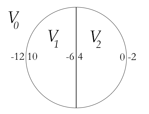
To find the second embedding of the dual in a rational surface, index the curves in the dual cycle by with , , , and meets , meets . Note generally that if there is a curve meeting , then contracting it and then leads to a surface and a nodal curve of square on . Thus must be either or . The case of is the case considered above. In case , there is obviously a root for (the proper transform of the curve on ). Also, one checks that the span an index two sublattice of and that is spanned by , with and . One can show that in fact both and are roots. It follows that there are infinitely many roots, and hence is infinite as well. The set is equal to . It is straightforward to check that , the reflection group generated by the roots, and all of the with are conjugate under . This case then corresponds to the case where is either or .
To sum up, we see that within each deformation type, there is exactly one combinatorial possibility for and exactly one element of square in . So Conjecture 5.14 is true in this case for classes of square .
6 Asymptotic behavior of the period map
Let be a Type III degeneration of anticanonical pairs. Fix a coordinate on and let be the corresponding coordinate on the universal cover . Thus and is well-defined on . As usual, let and let be the restriction of . Then is a local system with unipotent monodromy , which we denote by . Let . Note that the pullback of is trivialized by the choice of a point : is isomorphic to the constant sheaf with fiber .
The associated flat vector bundle has the canonical extension of Deligne [4]: can be taken to be the trivial holomorphic vector bundle , with the connection . A (local) flat section over is then a section locally of the form , for . In particular, we see that:
Proposition 6.1.
Let be a holomorphic section of . Then extends to a holomorphic section of if and only if, writing as a holomorphic function on with values in , the function , viewed as a function on , extends to a (single-valued) holomorphic function on with values in . ∎
On the other hand, by [35] (see also [4], [31]), the canonical extension is also given by . By Corollary 2.22, the subsheaf is a rank one subbundle of . An easy argument shows that, for , if , then (including the case ). We uniquely define an everywhere generating holomorphic section of by the requirement that
Now fix an integral splitting of the exact sequence
so that every element of is uniquely written as , where maps to the (oriented) generator of and . Note that, for , , and in particular , where we identify with its Poincaré dual. With our choice of , we can write
where is a multi-valued section of . By Proposition 6.1, the section extends to a single-valued holomorphic function on with values in . As
we see that
where is a single valued holomorphic function on with values in which extends to a holomorphic function on .
Thus , or equivalently:
Proposition 6.2.
, where and is holomorphic at . ∎
We then have the following corollary, which is a partial strengthening of [27, III(2.12)]:
Corollary 6.3.
The real, single-valued function with values in satisfies: for , , and in fact is in .
Proof.
We have
where is a function. The function is positive and tends to when , and hence extends to a continuous function on with . Thus for all . With our sign conventions, it follows that . Moreover, . Since is open in , for , . Thus, for , . ∎
Remark 6.4.
There is a several variable version of the above. The poldisk has boundary components, defined by , where is the coordinate on the factor. Given , such that the generic fiber over each boundary component is -semistable, there is an associated monodromy transformation with and . Then the period has the form
where is holomorphic.
By applying semistable reduction to a one parameter family over a disk which has order of contact with the component of the boundary, it follows that, for all , , we have (. This easily implies that, for , , and hence either for all or for all . Choosing orientations so that for all , it follows that, if for every , then .
7 The differential of the period map
We begin by discussing the smooth case, using [9] as a general reference. Let be an anticanonical pair (with a fixed orientation of ). For notational simplicity, we assume that each component of is smooth, i.e. that ; minor modifications handle the case . The period homomorphism is the homomorphism defined by: if and is the corresponding line bundle, then , and the period map is the map . The period map is holomorphic: for a fixed , given a family of pairs over , after shrinking we can assume that extends to a holomorphic line bundle over and that . The line bundle then defines a holomorphic map from to , and fitting these together for each defines the period map as a holomorphic map . The relationship between this period map and that considered in the previous section is as follows [9, (3.12)]:
The differential of the period map (for the semi-universal family) is then a map
We would like to describe the map . A local calculation shows:
Lemma 7.1.
Let be the composition of normalization and inclusion. Then there is an exact sequence
Given a line bundle on such that for every , its Chern class and its image in is zero. Thus, from the exact sequence
we see that lifts to a unique element of , which we denote by . Note that and we can think of as a Chern class with values in . The differential of the period map is then described as follows:
Theorem 7.2.
Let be the coboundary map arising from the exact sequence
which is an isomorphism since . Then
where denotes the cup product
Corollary 7.3.
is an isomorphism.
Proof.
Remark 7.4.
The vector space is dual to . Furthermore, is canonically isomorphic to . This gives the usual form of the differential of the period map, via cup product and contraction:
Proof of Theorem 7.2.
The class corresponds to a first order deformation . Explicitly, the correspondence is as follows: For a sufficiently small open cover of , there exists an isomorphism . Moreover, on , , where is a -cocycle. The condition that we keep the normal crossings divisor means that, in local coordinates,
for some holomorphic functions , , i.e. that is a section of over . However, in our situation we can do a little better:
Lemma 7.5.
After possibly shrinking the cover and modifying by a coboundary, we can assume that , i.e. that has the local form for some holomorphic functions , .
Proof.
We have a commutative diagram
A diagram chase shows that is surjective. Hence there is an exact sequence
But an easy calculation gives (i.e. every locally trivial deformation of is a product). Thus the natural map is surjective, which is the statement of the lemma. ∎
Returning to the proof of Theorem 7.2, fix once and for all a representative for satisfying the conclusion of the lemma. We have the usual exact sequence
and hence since . Hence, given a line bundle on , lifts uniquely to a line bundle on , which we see explicitly as follows: Every lifting of to an element of is necessarily of the form for some holomorphic functions . The condition that can be chosen to be a -cocycle is the equality
where is the -cochain and here and for the rest of the proof denotes Čech coboundary. In other words, the -cocycle is zero in . In this case, the transition functions
define the lift of to . Moreover, is then a -cocycle since
and, in case for , then represents the element .
We compute by lifting to a -cochain with values in and taking its Čech coboundary. Clearly, is such a lift, and thus is represented by the -cocycle .
Finally we compute the term . We can write
where is a -cocycle with values in representing and is a -cochain with values in . Thus is represented by the -cocycle
But, since ,
Since vanishes on , is a -coboundary with coefficients in . Thus, in cohomology, as claimed. ∎
We turn now to the case of a Type III degeneration . We define and by analogy with the smooth case:
Note that, by Lemma 2.20,
Lemma 7.6.
.
Proof.
We have the analogue of the exact sequence of Lemma 7.1:
Thus there is an exact sequence
This identifies with the kernel of
which is . ∎
There is a period homomorphism and it extends to a holomorphic map on germs of deformations of . In particular, there is a well-defined differential
To compute it, note first that the analogue of Lemma 7.1 holds, so that given , we have and its image . Then we have
Theorem 7.7.
Let be the coboundary map arising from the exact sequence
which is an isomorphism since . Then
where denotes Yoneda pairing
Proof.
On the hyperplane of , the Yoneda product is just cup product, and the proof is exactly the same as the proof for Theorem 7.2. By linearity, it suffices to prove the formula of Theorem 7.7 for a single class projecting onto a nonzero element of . Fix a one parameter smoothing . There are relative versions , , , . We also have the relative Kodaira-Spencer map , and is a section which restricts to an element with nonzero image in . Given , we can lift to a line bundle , and there is a relative (modified) Chern class . We want to establish the equality
This holds for a general by Theorem 7.2, and thus follows by continuity for , noting that is torsion free (see also Proposition 8.7 below). Restricting to gives the result for . ∎
Remark 7.8.
We will only need this result for , the hyperplane tangent to the equisingular deformations.
Corollary 7.9.
The restriction of the differential of the period map to is an isomorphism and the differential of the period map on is surjective.
Proof.
Note that , and similarly for . Thus there is the cup product map
which is identified via with
the differential of the period map. By [6, (2.10)], the vector spaces and are dual under cup product, hence the above cup product is nondegenerate by Serre duality. Moreover by compatibility of cup product,
where is the image of . This proves the first statement and the second then follows. ∎
8 Surjectivity of the period map
In this section, our goal is to use Theorem 7.7 to prove results about the surjectivity of the period map for families of -semistable Type III anticanonical pairs, and then to apply this to construct Type III degenerations such that the kernel of the period map on a general fiber is of a special type.
Let be a Type III anticanonical pair as defined in Definition 2.1. If is the central fiber of a Type III degeneration of anticanonical pairs, which is the case if and only if is -semistable, then there are line bundles on , namely , . By Lemma 2.16,
Define a class by the rule:
By the triple point formula, , and hence . It is easy to check that . Clearly for every component of .
Lemma 8.1.
The homomorphism defined by
has kernel and thus defines an injective homomorphism . Moreover, the cokernel of is torsion free.
Proof.
Suppose that is in the kernel. After adding the element , we may assume that and must show that for all . We have in . As the classes are linearly independent in , for all such that . Fix one such component . Then there exists a component such that , corresponding to a triple point of lying on . By assumption, in , and . An easy argument (cf. [9, 2.8]) shows that, if is an anticanonical pair and is a chain of length , i.e. , , then the classes are linearly independent in . Applying this fact to the pair , it follows that for all such that . Continuing in this way and using the fact that the dual complex of is connected, a straightforward argument then shows that for all .
Finally, we must show that is torsion free. This statement is invariant under a locally trivial deformation, so we can assume that is -semistable by [10, (2.16)], and that is a smoothing. Thus as described above. The proof of (i) of Proposition 3.9 shows that there is an inclusion of in for a general fiber . Hence is torsion free. ∎
We next define the period map for -semistable Type III anticanonical pairs:
Definition 8.2.
Let be the lattice defined by
Note that the condition is well-defined since for all and . By the proof of Lemma 8.1, if is -semistable and is a smoothing, then there is an inclusion of in for a general fiber .
For a Type III anticanonical pair , with oriented, we have the period map defined by . If is -semistable, then clearly for every . We define to be the homomorphism induced by . Given a locally trivial deformation of the pair with trivial monodromy, over a smooth connected base , with all fibers -semistable, there exists a holomorphic map in the usual way.
The following is then the main result of this section:
Theorem 8.3.
Let be a homomorphism. Then there exists a locally trivial deformation of with trivial monodromy, over a smooth connected base which we can take to be of the form , such that all fibers are -semistable, and a point such that, if is the corresponding Type III anticanonical pair, then for all and the induced homomorphism is .
Proof.
There are three ways that we can deform in a locally trivial way (cf. [11, (4.3)] for more details):
- 1.
We change the gluings by multiplying by .
- 2.
If is obtained by blowing up a point , we can deform the point to a point . (Note that a blowup at a singular point of the anticanonical divisor has no moduli.)
- 3.
In most cases, is obtained via iterated blowups from a minimal pair with no moduli (taut, in the terminology of [9]). In a very small number of exceptional cases ( or is already minimal and the double curve on is either irreducible nodal or has two components of self-intersection ), the pair has moduli .
There is then a “universal” deformation of , parametrized by , corresponding to the different possibilities (1), (2), (3) above. Universal in this sense simply means that every locally trivial deformation of appears as a fiber. After a translation on , we can assume that corresponds to . Furthermore, the monodromy of the family is trivial. Finally, we can assume that there is a unique component of isomorphic to .
Let be the double curve on . Then it is easy to check that is rigid under locally trivial deformations and that . Furthermore, if denotes the neutral component of , then . Since , as well, and thus we can choose an isomorphism of schemes
Since the monodromy of the family is trivial, there is a period map .
Lemma 8.4.
Let be the deformation constructed above. Then the period map is an affine map of tori.
Proof.
Very generally, if is a morphism of algebraic varieties, then by a theorem of Rosenlicht is an affine map. We will give an essentially direct argument that is an affine map. Thus, given a line bundle on , we must analyze how varies as we vary the gluings.
Let be the dual cycle to on . As previously noted, , and hence
Thus, an orientation on induces a compatible orientation on , and
In particular, if is a line bundle on which restricts to a line bundle of multidegree on , then the map is an affine isomorphism from to .
Choose an ordering on the components of so that , , i.e. , where the ordering of the components of is compatible with the orientation. Let . Then Mayer-Vietoris applied to the union implies that there is an exact sequence
i.e. a line bundle on is determined by line bundles on and on , such that , where is the isomorphism given by . Thus, if , and the gluing changes by , where is given by a surjective homomorphism from to a subtorus of , then the line bundle deforms to some line bundle corresponding to pairs , the line bundle corresponding to over the corresponding deformation of and , with , such that
If , where the factor operates in the usual way on the component of , then acts trivially on , and acts on , the set of line bundles on of multidegree , via and the usual action of on . Given and , there is a unique line bundle for which the compatibility condition holds. Thus, if we can show that is an affine map, it follows that is affine and hence so is , where is the class corresponding to the line bundle .
The line bundle determines a multidegree , with , and hence , . Restriction defines a morphism , and it is equivariant with respect to the actions of on and on via the natural homomorphism . We now consider the various ways that the construction of Lemma 8.5 changes the line bundle :
- 1.
Suppose that we change the gluings by . Here we may assume that since we have already dealt with the gluings from to . The line bundle is then replaced by for the automorphism corresponding to multiplying by on the component .
- 2.
If is obtained by blowing up a point , and we replace by , then the line bundle is then replaced by for an appropriate integer .
- 3.
In this exceptional case, a direct if somewhat tedious calculation shows that the corresponding map is affine (cf. [11, Lemma 4.6]). Alternatively, it is clear that the map is a morphism (i.e. algebraic) and hence it is affine by Rosenlicht’s theorem.
Combining the various possibilities, we see that we get an affine map from to as claimed. ∎
Consider the affine map defined by
where we view the image of as contained in the subtorus defined by: the product of the components is . Let be the neutral component of .
Lemma 8.5.
Let be the restriction of the family to the subtorus of . Then:
- (i)
For all , is -semistable.
- (ii)
The image of the Kodaira-Spencer map is
Proof.
By arguments similar to the proof of Lemma 8.4, one checks that defined by is an affine map and hence a homomorphism. By definition, the locus of -semistable deformations is . Then both and are homomorphisms since they take the identity to the identity, and . The differential of is surjective at by construction and [6, (5.9) and (4.5)]. Hence the codimension of is . The differential of is also surjective by Corollary 7.9. Hence . Thus the two subtori and have the same tangent space at and hence are equal. In particular, all fibers are -semistable. The final statement (ii) about the Kodaira-Spencer map then follows from Theorem 7.7. ∎
To complete the proof of Theorem 8.3, consider the family described in the remarks before Lemma 8.5. By construction, the family induces a period map . By Lemma 8.4, the map is an affine map. We claim that the differential of is surjective. By Lemma 8.5 and the remarks before it, we are reduced to showing the following: let
be defined as . We can replace by in the above. Moreover,
Then cup product induces a perfect pairing
This says that the differential of is surjective. Hence is an affine map of tori with surjective differential. It follows that is surjective. This is exactly the statement of Theorem 8.3. ∎
Remark 8.6.
Related methods give a somewhat more direct proof of Theorem 4.1 in [11].
We can relate the period map for a -semistable Type III anticanonical pair to the period map for nearby smoothings as follows. Suppose that is a morphism from the smooth complex manifold to the polydisk, whose fibers are smooth anticanonical pairs for and such that the fibers over are -semistable Type III anticanonical pairs. We will apply this in the case of the germ of the smoothing component of a -semistable Type III anticanonical pair below and for one parameter families (the case ) in Section 9. In this case, the monodromy on is trivial, there is a well-defined monodromy invariant , and there is an inclusion identifying the image with .
Proposition 8.7.
Let denote restriction. The function defined by
is holomorphic.
Proof.
For a fixed , there is a corresponding line bundle on , well defined up to twisting by components of the inverse image of . Restricting to and choosing a trivialization (which is always possible locally) gives a holomorphic map . By definition, this map is independent of the choice of and defines , evaluated on the class . Doing this construction for a basis of shows that is holomorphic. ∎
Remark 8.8.
Using the alternative formulation of the period map from the preceding section and Proposition 6.2 in the parametrized case, we see that, if is a coordinate defining the last factor of in the notation above, and is a class in , then, for ,
where extends to a holomorphic, nowhere zero function on . Hence, extends to a holomorphic function on with values in .
We will then need the following, which is in a sense complementary to Theorem 8.3:
Proposition 8.9.
Suppose that is a -semistable Type III anticanonical pair. Let be a sublattice of such that for all . Then there exists a Type III degeneration , with special fiber such that, via the specialization map
for all .
Proof.
Let be the germ of the subspace of the semiuniversal deformation of the pair corresponding to the smoothing component and, on the discriminant locus, to preserving the condition of -semistability. Note that and that the classes extend to Cartier divisors on with trivial restriction to . By Proposition 8.7, there is a well-defined, holomorphic period map (on the level of germs) . Via restriction, there is a surjection
and in particular the differential of the surjection is also surjective. Taking the composition with the period map, there is a (germ of a) holomorphic map . Theorem 7.7 and Corollary 7.9 imply that is a submersion at and that is transverse to the discriminant hypersurface. Taking a generic map of the disk to (and which is in particular transverse to the discriminant) gives the existence of the Type III degeneration above. ∎
9 Good sublattices and adjacent RDP singularities
Throughout this section, we fix a deformation type of a negative definite anticanonical pair , and denotes the set of roots of . We begin by describing a class of negative definite sublattices of :
Lemma 9.1.
Let be an anticanonical pair and let be a negative definite sublattice of , not necessarily primitive. Suppose that
- (i)
is spanned by elements of .
- (ii)
The period homomorphism satisfies: .
Then is a root system in the real vector space and there exist a set of simple roots such that
- (i)
For every , , where is a -curve.
- (ii)
If and , then , where the are nonnegative integers. In particular, if is a -curve on , then for some .
Proof.
If , then by [9, (6.9)]. It then follows e.g. by Definition 1 in [2, IV §1] that is a root system in (and in fact that every element of square in the -span of is a root).
Let be the set of -curves on , let be the reflection group generated by , and let . Then, by [9, Theorem 6.6], . Let be the simple roots for a Weyl chamber in defined by an ample divisor on . By [8, Lemma 2.4(ii)], all positive roots are effective. On the other hand, every is of the form , where the are -curves on . A standard argument using the fact that is negative definite shows that, if is effective and of the form , where the are -curves, then for all . Hence the positive roots are exactly the classes of the of the form , , and the simple roots are exactly the classes of the -curves on . ∎
Lemma 9.2.
Let be a negative definite sublattice of and suppose that is spanned by . Then there exists a such that .
Proof.
Let be the saturation of , and let be the finite index sublattice of spanned by . Then there exists a with . Hence , and is spanned by . Using the surjectivity of the period map, there exists a such that . By Lemma 9.1, there exist -curves whose classes span . Moreover, there is a nef and big divisor on such that for all , for all and for every curve or . If , then and for all , hence for all . ∎
We can then rephrase the conditions of Lemma 9.1 as follows:
Lemma 9.3.
Let be a class in . Let , . Suppose that . Then .
Hence, the condition (i) of Lemma 9.1 is equivalent to: there exists a such that and
(i)′ is spanned by elements of of square .
Proof.
Since is in the interior of , it is easy to check that is not orthogonal to any exceptional curve and hence that there is a neighborhood of in which is disjoint from for every exceptional curve . There exist positive such that for all , and hence
for all . Multiplying the by a positive , we can further assume that is not separated from by a wall of the form , where is exceptional, and hence . Thus meets the interior of . It follows from [9, Theorem 6.6] that . ∎
Definition 9.4.
Let be a negative definite sublattice of , not necessarily primitive. Then is good if
- (i)
is spanned by elements of .
- (ii)
There exists a homomorphism such that .
The lattice determines an RDP configuration (possibly consisting of more than one singular point) by taking the appropriate type of a set of simple roots for . We say that the corresponding RDP configuration is of type .
Given , the lattice is -good if it is good and if . By Lemma 9.2, every good sublattice is -good for some .
Let be a lattice spanned by elements of . If is primitive, then it is good. If is the saturation of and is cyclic, then is good. If is the decomposition of into its irreducible summands, then is good is good for every (this follows easily from the fact that, if with for all and if , then for some and ).
To explain the geometric meaning of good lattices, we start with the following definition:
Definition 9.5.
A generalized anticanonical pair is a pair , where is a rational surface, possibly with rational double points, and is a cycle contained in the smooth locus of , such that, if is the minimal resolution, then is an anticanonical pair.
We then have the following alternate characterization of RDP configurations of type (cf. [27, II (2.7)]):
Proposition 9.6.
Suppose that is a generalized anticanonical pair with minimal resolution such that every -curve on is contained in a fiber of . Then the classes of the components of fibers of generate a good sublattice of , and every good sublattice of arises in this way.
Hence the RDP configurations of type , for some good sublattice of , are exactly the RDP configurations which appear on a generalized anticanonical pair whose minimal resolution has deformation type and which satisfy the condition that every -curve on the minimal resolution is contained in a fiber of .
Proof.
If is as in the statement of the proposition, let . Then, by [9, 6.6] and its method of proof, , where is a -curve on . Thus . It follows that is a negative definite lattice spanned by , so that is good.
Conversely, suppose that is a good sublattice. By the surjectivity of the period map, we can choose an anticanonical pair such that and is spanned by . By Lemma 9.1, there exists a set of simple roots , where the are exactly the -curves on . Since is negative definite, there exists a morphism , where is normal and exactly contracts the . Hence is a generalized anticanonical pair with minimal resolution such that every -curve on is contained in a fiber of . ∎
We now relate the above discussion to the existence of adjacent RDP singularities.
Theorem 9.7.
Let be a Type III degeneration with monodromy invariant . Let be the finite set of elements of such that . Then, for all , and for all , for some and the function is identically equal to for all .
Proof.
: Obvious.
: Let be a neighborhood of in such that, if and is a wall with , then for some , i.e. is one of the finitely many walls corresponding to elements of and passing through .
Given , the function is a well-defined, function on and thus corresponds to a function , which we continue to denote by . By [9, (3.12)],
as multi-valued functions on . Hence, by Proposition 6.2,
for a single-valued holomorphic function which extends to a holomorphic function at . Taking real parts, we obtain an equality of (single-valued) functions
where is a function at . Dividing by gives
Thus defines a continuous function with . Thus, for , . It follows that, if , , , and , then lies on and so for some .
Given as above, either is identically equal to for all or for at most finitely many . Choosing smaller if need be, we can then assume that, for all , if is not identically equal to , then for all . ∎
Given a Type III degeneration , by a theorem of Shepherd-Barron [34, Theorem 2A, p. 157], there exists a birational morphism over , where contracts and the cycle to a point and, for , is the minimal resolution of a union of rational double points. We then have the following (compare [27, III (2.12)]):
Proposition 9.8.
For , the irreducible components of the exceptional fibers of are exactly the -curves on .
Proof.
Clearly, if is an irreducible component of an exceptional fiber of , then is a -curve on . Conversely, suppose that is a -curve on for some for and let . Then . By Theorem 9.7, is orthogonal to and is identically . It follows from Proposition 3.9 that corresponds to a line bundle on . For all , , i.e. where the are -curves on . The condition on that is effective on is closed (by semicontinuity) and open (because we can choose a relatively ample divisor on over small open subsets of ). Since is effective on , it follows that is effective for all , and, for generic, is the class of an irreducible curve. Since for all , arguing as in the proof of Proposition 3.11, after modifying by , we can assume that where is a surface on , not containing for any , and such that . In particular, there exists an effective Cartier divisor on such that for every . But every such divisor is a sum of the form , where , plus components disjoint from , and hence is contained in . Since is negative definite, this is only possible if for all . Thus , so that, via the relative contraction morphism over , is contracted to a point. Since fibers over and contracts the fiber to a point, must contract all fibers of to points as well. Thus contracts to a point. ∎
We can now state the main result concerning possible adjacencies of the cusp to RDP singularities:
Theorem 9.9.
(i) Suppose that and that is a -good sublattice of . Let be a Type III anticanonical pair of type . Then the cusp is adjacent to an RDP configuration of type . More precisely, after a locally trivial deformation of through -semistable varieties, there exists a Type III degeneration with central fiber and a blowdown over , such that the central fiber of is with contracted and the singular locus of the general fiber is an RDP configuration of type .
(ii) Conversely, suppose that the cusp is adjacent to an RDP configuration via a one parameter family of -type . For , if is the minimal resolution of a general fiber of , then the components of the exceptional curves generate a -good sublattice of , and the RDP configuration on the general fiber is of type .
Proof.
(i) Given the -good sublattice , choose a such that . Let be the restriction of to . By Theorem 8.3, after a locally trivial deformation of through -semistable varieties, we can assume that . By Proposition 8.9, there exists a Type III degeneration with central fiber such that, under the natural identification of and with sublattices of , for all and all . Conversely, by Theorem 9.7, for , if and , then is identically and , hence . Using the continuity of (Proposition 8.7), as well. Thus . In particular, by Lemma 9.1, the -curves on correspond to a set of simple roots for . By Proposition 9.8, these are exactly the exceptional fibers of the blowdown . Hence the singular locus of is an RDP configuration of type .
(ii) After a base change, we can assume that is birational to a Type III degeneration of -type . For , let be the sublattice of generated by . By Theorem 9.7, if , then , and hence . Thus is good, in fact it is -good. By Lemma 9.1, the classes of the -curves on are a set of simple roots for . By Proposition 9.8, the -curves on are exactly the fibers of the morphism . Hence the RDP configuration on is of type . ∎
Corollary 9.10.
Let be a cusp singularity with minimal resolution and let be the dual cycle. Suppose that is an anticanonical pair. Then the possible nearby RDP configurations on some smoothing component of of type are exactly the RDP configurations of type , where is a good sublattice of .
Proof.
Suppose that there is a nearby RDP configuration on some smoothing component of of type . Then we can choose a one parameter deformation , where the central fiber is the Inoue surface with contracted. After base change, there is a birational model for which is a Type III degeneration with monodromy invariant for some . By (ii) of Theorem 9.9, the RDP configuration on a general fiber of is of type , where is a -good and hence good sublattice of .
References
- [1] M. Abouzaid, D. Auroux, and L. Katzarkov, Lagrangian fibrations on blowups of toric varieties and mirror symmetry for hypersurfaces, https://arxiv.org/abs/1205.0053, 2012.
- [2] N. Bourbaki, Groupes et Algèbres de Lie, Chap. 4, 5, et 6, Masson, Paris, 1981.
- [3] C.H. Clemens, Jr., Picard-Lefschetz theorem for families of nonsingular algebraic varieties acquiring ordinary singularities, Trans. Amer. Math. Soc. 136 (1969), 93–108.
- [4] P. Deligne, Équations différentielles à points singuliers réguliers, Lecture Notes in Mathematics, Vol. 163. Springer-Verlag, Berlin-New York, 1970.
- [5] P. Engel, A proof of Looijenga’s conjecture via integral-affine geometry, http://arxiv.org/pdf/1409.7676, 2014.
- [6] R. Friedman, Global smoothing of varieties with normal crossings, Annals of Math. 118 (1983), 75–114.
- [7] R. Friedman, Base change, automorphisms, and stable reduction for type III surfaces, in The Birational Geometry of Degenerations pp. 277–298, Progr. Math. 29, Birkhäuser, Boston, Mass., 1983.
- [8] R. Friedman, On the ample cone of a rational surface with an anticanonical cycle, Algebra & Number Theory 7 (2013), 1481–1504.
- [9] R. Friedman, On the geometry of anticanonical pairs, arxiv.org/abs/1502.02560, 2016.
- [10] R. Friedman and R. Miranda, Smoothing cusp singularities of small length, Math. Ann. 263 (1983), 185–212.
- [11] R. Friedman and F. Scattone, Type III degenerations of surfaces, Invent. Math. 83 (1986), 1–39.
- [12] M. Gross. Special Lagrangian fibrations I: Topology, https://arxiv.org/abs/alg-geom/9710006, 1997.
- [13] M. Gross, P. Hacking, and S. Keel, Moduli of surfaces with an anti-canonical cycle, Compos. Math. 151 (2015), 265–291.
- [14] M. Gross, P. Hacking, and S. Keel, Mirror symmetry for log Calabi-Yau surfaces I, Publ. Math. Inst. Hautes Études Sci. 122 (2015), 65–168.
- [15] M. Gross and B. Siebert, Mirror symmetry via logarithmic degeneration data I, J. of Differential Geom. 72.2 (2006), 169–338.
- [16] M. Gross and B. Siebert. Mirror symmetry via logarithmic degeneration data, II. J. of Algebraic Geom. 19.4 (2010), 679–780.
- [17] N. Hitchin, The moduli space of special Lagrangian sub manifolds, Annali Scuola Sup. Norm. Pisa Sci. Fis. Mat. 25 (1997), 503–515.
- [18] M. Inoue, New surfaces with no meromorphic functions II, in Complex analysis and algebraic geometry, 91–106. Iwanami Shoten, Tokyo, 1977.
- [19] Y. Kawamata and Y. Namikawa, Logarithmic deformation of normal crossing varieties and smoothing of degenerate Calabi-Yau manifolds, Invent. Math. 118 (1994), 395–409.
- [20] M. Kontsevich, Homological algebra of mirror symmetry, https://arxiv.org/abs/alg-geom/9411018, 1994.
- [21] M. Kontsevich and Y. Soibelman. Affine structures and non-Archimedean analytic spaces, The unity of mathematics, Birkhäuser Boston (2006), 321–385.
- [22] C. L. Lawson, Transformation triangulations Discrete Math. 3 (1972), 365-272.
- [23] T.-J. Li and A.-K. Liu, Uniqueness of symplectic canonical class, surface cone and symplectic cone of 4-manifolds with , J. Differential Geom. 58 (2001), 331–370.
- [24] T.-J. Li and C. Y. Mak, Symplectic log Calabi-Yau surface—deformation class, http://arxiv.org/pdf/1510.06131, 2015.
- [25] E. Looijenga, On the semi-universal deformation of a simple-elliptic hypersurface singularity. II. The discriminant, Topology 17 (1978), 23–40.
- [26] E. Looijenga, The smoothing components of a triangle singularity. II, Math. Ann. 269 (1984), 357–387.
- [27] E. Looijenga, Rational surfaces with an anti-canonical cycle, Annals of Math. 114 (1981), 267–322.
- [28] E. Looijenga and J. Wahl, Quadratic functions and smoothing surface singularities, Topology 25 (1986), 261–291.
- [29] D. Morrison. Compactifications of moduli spaces inspired by mirror symmetry, https://arxiv.org/abs/alg-geom/9304007, 1993.
- [30] U. Persson, On Degenerations of Algebraic Surfaces, Mem. Amer. Math. Soc. 11 (1977), no. 189.
- [31] C.A.M. Peters and J.H.M. Steenbrink, Mixed Hodge structures, Ergebnisse der Mathematik und ihrer Grenzgebiete, 3. Folge, 52. Springer-Verlag, Berlin, 2008.
- [32] H. C. Pinkham, Simple elliptic singularities, Del Pezzo surfaces and Cremona transformations, in Several complex variables (Proc. Sympos. Pure Math., Vol. XXX, Part 1, Williams Coll., Williamstown, Mass., 1975), 69–71. Amer. Math. Soc., Providence, R. I., 1977.
- [33] H. C. Pinkham, Groupe de monodromie des singularités unimodulaires exceptionnelles, C. R. Acad. Sci. Paris Sér. A-B 284 (1977), A1515–A1518.
- [34] N. I. Shepherd-Barron, Extending polarizations on families of surfaces, in The Birational Geometry of Degenerations pp. 135–171, Progr. Math. 29, Birkhäuser, Boston, Mass., 1983.
- [35] J.H.M Steenbrink, Limits of Hodge structures, Invent. Math. 31 (1975/76), 229–257.
- [36] A. Strominger, S.-T. Yau, and E. Zaslow, Mirror symmetry is T-duality. Nuclear Physics B 479.1-2 (1996), 243–259.
- [37] M. Symington, Four dimensions from two in symplectic topology, in Proceedings of Symposia in Pure Mathematics, Vol. 71, pp. 153–208. Amer. Math. Soc., 2003.
- [38] J. Wahl, Elliptic deformations of minimally elliptic singularities, Math. Ann. 253 (1980), 241–262.
Philip Engel
Department of Mathematics
Harvard University
Cambridge, MA 02138
USA
engel@math.harvard.edu
Robert Friedman
Department of Mathematics
Columbia University
New York, NY 10027
USA
rf@math.columbia.edu