跳到论文正文
W Papers独立论文阅读器 arXiv:1609.07978 论文正文 计算阅读时间 · 0%
引用这篇论文根据当前论文元数据生成,正式投稿前建议核对。


License: arXiv.org perpetual non-exclusive license
arXiv:1609.07978v1 [cs.IT] 26 Sep 2016

Antenna Selection for MIMO-NOMA Networks

Yuehua Yu Affiliation: School of Electrical and Information Engineering, The University of Sydney, Australia*School of Computing and Communications, Lancaster University, UK    He Chen Affiliation: School of Electrical and Information Engineering, The University of Sydney, Australia*School of Computing and Communications, Lancaster University, UK    Yonghui Li Affiliation: School of Electrical and Information Engineering, The University of Sydney, Australia*School of Computing and Communications, Lancaster University, UK    Zhiguo Ding*    Branka Vucetic Affiliation: School of Electrical and Information Engineering, The University of Sydney, Australia*School of Computing and Communications, Lancaster University, UK    Email: {yuehua.yu Affiliation: School of Electrical and Information Engineering, The University of Sydney, Australia*School of Computing and Communications, Lancaster University, UK    he.chen    yonghui.li    branka.vucetic}@sydney.edu.au    *z. ding@lancaster.ac.uk
Abstract

This paper considers the joint antenna selection (AS) problem for a classical two-user non-orthogonal multiple access (NOMA) network where both the base station and users are equipped with multiple antennas. Since the exhaustive-search-based optimal AS scheme is computationally prohibitive when the number of antennas is large, two computationally efficient joint AS algorithms, namely max-min-max AS (AIA-AS) and max-max-max AS (A3-AS), are proposed to maximize the system sum-rate. The asymptotic closed-form expressions for the average sum-rates for both AIA-AS and A3-AS are derived in the high signal-to-noise ratio (SNR) regime, respectively. Numerical results demonstrate that both AIA-AS and A3-AS can yield significant performance gains over comparable schemes. Furthermore, AIA-AS can provide better user fairness, while the A3-AS scheme can achieve the near-optimal sum-rate performance.

I Introduction

The non-orthogonal multiple access (NOMA) technique has been recently regarded as a promising solution to significantly improve the spectral efficiency of 5G wireless networks [1]. By superposing the information of multiple users in the power domain, multiple users can be served within the same time, frequency and code domain. Different from the conventional water-filling power allocation strategy, the NOMA technique allocates more transmit power to the users with poor channel conditions (i.e., weak users). In this case, these users can decode their higher-power-level signals directly by treating others’ signals as noise. In contrast, those users with better channel conditions (i.e., strong users) adopt the successive interference cancellation (SIC) technique for signal detection. Specifically, the weak users’ messages are first decoded and subtracted before the strong users’ massages with lower-power-levels can be recovered. It has been demonstrated that both the system throughput and user fairness are significantly improved in NOMA systems compared to conventional orthogonal multiple access (OMA) systems [1].

Recent works have attempted to apply the multiple-input-multiple-output (MIMO) techniques into NOMA systems (MIMO-NOMA) to exploit the spatial degrees of freedom [2, 3, 4]. Although the capacity performance can potentially scale up with the increase of the number of antennas, this superior performance comes at the price of expensive RF chains at terminals. To avoid the heavy burden of hardware expenses while preserving the diversity benefits from MIMO, the antenna selection (AS) technique has been well recognized as an effective solution [5]. There are only a few papers that considered the AS problem for MIMO-NOMA systems in open literature. Specifically, a transmit AS (TAS) algorithm was proposed in [6], and a joint TAS and user scheduling algorithm was studied in [7]. However, both [6] and [7] only focused on the TAS design at the base station side as each user was assumed to equipped with single antenna. Moreover, the insightful analytical expressions of the system performance have not been derived in [6] and [7].

To our best knowledge, the joint AS at both the base station and users for MIMO-NOMA systems is still an open problem. Though there are some previous literatures which studied the joint AS schemes in conventional MIMO-OMA systems, they cannot be extended to MIMO-NOMA systems directly. This is because there are severe inter-user interferences in MIMO-NOMA systems while the signals are transmitted in an interference free manner in MIMO-OMA systems. A native way to find the global optimal solution of the problem may require an exhaustive search (ES) over all possible antenna combinations, whose complexity would become unacceptable as the numbers of antennas at both the base station and users become large. Motivated by this, in this paper we propose two computationally efficient joint AS algorithms for MIMO-NOMA systems, namely max-min-max AS (AIA-AS) and max-max-max AS (A3-AS), to maximize the system sum-rate. Specifically, AIA-AS tries to improve the performance of the instantaneous weak user while the A3-AS scheme maximizes the performance of the instantaneous strong user. The asymptotic closed-form expressions for the average rates for both AIA-AS and A3-AS are derived for high signal-to-noise (SNR) scenario. All analytical results are validated by computer simulations and it is demonstrated that both the AIA-AS and A3-AS can yield significant performance gains over comparable schemes. Furthermore, AIA-AS can provide better user fairness while the A3-AS scheme can achieve the near-optimal sum-rate performance.

II System Model
Refer to caption
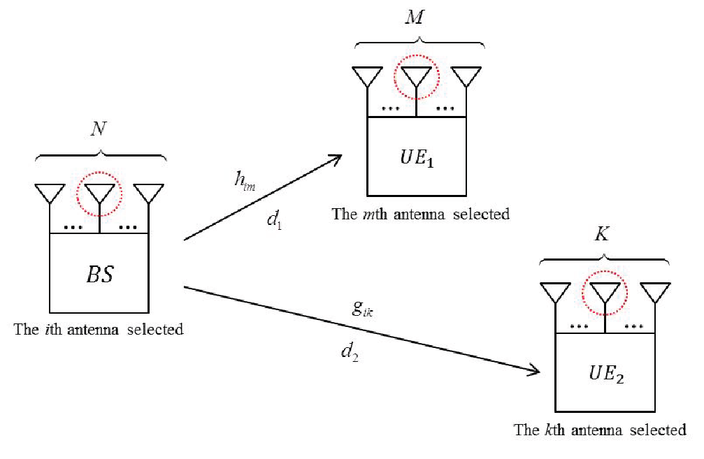
Fig. 1: Diagram of a MIMO-NOMA down-link scenario with multiple antennas at each node.

Consider a two-user MIMO-NOMA down-link scenario, since the two-user scenario is how NOMA is implemented in LTE-Advanced [3]. As shown in Fig. 1, the base station (BS) is equipped with NN antennas, while user one (UE1) and user two (UE2) are equipped with MM and KK antennas, respectively. The channel matrix from the BS to UE1 is denoted by 𝐇∈𝒞N×M{\bf{H}}\in{\mathcal{C}^{N\times M}} and the one from the BS to UE2 is denoted by 𝐆∈𝒞N×K{\bf{G}}\in{\mathcal{C}^{N\times K}}, where 𝒞m×n\mathcal{C}^{m\times n} represents the set of all m×nm\times n matrices. We assume that the channels between the BS and users are spatially uncorrelated flat Raleigh fading, then the entries of 𝐇\mathbf{H} (𝐆\mathbf{G}), e.g., h~i​m{\tilde{h}_{im}} (g~i​k{\tilde{g}_{ik}}), can be modeled as independent and identically distributed (i.i.d.) complex Gaussian random variables, where h~i​m\tilde{h}_{im} (g~i​k\tilde{g}_{ik}) represents the channel coefficient between the iith antenna of the BS and the mmth (kkth) antenna of UE1 (UE2). Specially, we define hi​m=|h~i​m|2{h}_{im}=|\tilde{h}_{im}|^{2} and gi​k=|g~i​k|2{g}_{ik}=|\tilde{g}_{ik}|^{2}, where the operation |⋅|\left|{\cdot}\right| denotes the absolute value.

We assume all the nodes are limited with one RF chain based on the cost consideration. As such, in each resource block, the BS selects one (e.g., iith) out of NN available antennas to transmit information, while the users select one (e.g., mmth and kkth) out of MM and KK available antennas respectively to receive massages. To proceed, the global information of the channel amplitudes are assumed to be perfectly known at the BS.

Let δ\delta denote the indicator, defined as

δ={1,hi​m≥gi​k,0,hi​m<gi​k.\displaystyle\delta=\left\{{\begin{array}[]{*{20}{c}}{1,}&{{h}_{im}\geq{g}_{ik}},\\ {0,}&{{h}_{im}<{g}_{ik}}.\end{array}}\right.

According to the principle of NOMA, the BS broadcasts the signals superposed in the power domain as

x=(1−δ)​(a​s1+b​s2)+δ⁡(b​s1+a​s2),\displaystyle x=({1-\delta})(\sqrt{a}s_{1}+\sqrt{b}s_{2})+\delta(\sqrt{b}s_{1}+\sqrt{a}s_{2}), (4)

where sis_{i} denotes the signal to UEi with 𝔼⁡[|si|2]=1\mathbb{E}[{\left|{{s_{i}}}\right|^{2}}]=1 and 𝔼⁡[⋅]\mathbb{E}[\cdot] denotes the expectation operation. aa and bb are the power allocation coefficients satisfying a+b=1a+b=1. For notational simplicity, we assume that a>ba>b is set to guarantee that more power is allocated to the instantaneous weak user.

The received signals at UEs are given by

y1\displaystyle{y_{1}} =\displaystyle= Ps​h~i​m​x+n1,\displaystyle\sqrt{P_{s}}\tilde{h}_{im}x+n_{1}, (5)
y2\displaystyle{y_{2}} =\displaystyle= Ps​g~i​k​x+n2,\displaystyle\sqrt{P_{s}}\tilde{g}_{ik}x+n_{2}, (6)

where PsP_{s} is the transmit power at the BS, and nin_{i} is the complex additive white Gaussian noise (AWGN) with variance σi2\sigma_{i}^{2}. For simplicity, we assume σ12=σ22=σ2\sigma_{1}^{2}=\sigma_{2}^{2}=\sigma^{2}.

When δ=1\delta=1, UE2 is the weak user and UE1 is the strong user, hence the power level of s2s_{2} is larger than that of s1s_{1}. In this case, UE2 decodes s2s_{2} directly by treating s1s_{1} as noise. In contrast, UE1 first decodes s2s_{2} and subtracts it by performing SIC, then decodes its own s1s_{1} without interference. For the case δ=0\delta=0, the decoding order is inverted. By using the fact that the channels are ordered, it can be easily verified that SIC can be carried out successfully, and the following two rates are achievable to the users:

R1\displaystyle{R_{1}}\!\!\! =\displaystyle= (−δ)​log2⁡(+a​hi​mb​hi​m+1ρ)+δ​log2⁡(1+ρ​b​hi​m),\displaystyle\!\!\!\left(1\!-\!\delta\right)\log_{2}\left(1\!+\!\frac{a{h}_{im}}{b{h}_{im}+\frac{1}{\rho}}\right)\!+\!\delta\log_{2}\left(1+\rho b{h}_{im}\right), (7)
R2\displaystyle{R_{2}}\!\!\! =\displaystyle= (−δ)​log2⁡(+ρ​b​gi​k)+δ​log2⁡(1+a​gi​kb​gi​k+1ρ),\displaystyle\!\!\!\left(1\!-\!\delta\right)\log_{2}\left(1\!+\!\rho b{g}_{ik}\right)\!+\!\delta\log_{2}\left(1+\frac{a{g}_{ik}}{b{g}_{ik}+\frac{1}{\rho}}\right), (8)

where ρ=Ps​/​σ2{\rho}={{{P_{s}}}\mathord{\left/{\vphantom{{{P_{s}}}{{\sigma^{2}}}}}\right.\kern-1.2pt}{{\sigma^{2}}}} is the transmit SNR. Accordingly, the achievable system sum-rate is given by

Rsum\displaystyle R_{\mathrm{sum}} =\displaystyle= R1+R2\displaystyle R_{1}+R_{2} (9)
=\displaystyle= log2⁡(1+ρ​b​γ~is)+log2⁡(1+a​γ~iwb​γ~iw+1/ρ),\displaystyle\log_{2}\left(1+\rho b\tilde{\gamma}_{i}^{s}\right)+\log_{2}\left(1+\frac{a\tilde{\gamma}_{i}^{w}}{b\tilde{\gamma}_{i}^{w}+1/\rho}\right),

where γ~is=max⁡(hi​m,gi​k)\tilde{\gamma}_{i}^{s}=\max\left({h}_{im},{g}_{ik}\right) denotes the instantaneous channel gain of the strong user and γ~iw=min⁡(hi​m,gi​k)\tilde{\gamma}_{i}^{w}=\min\left({h}_{im},{g}_{ik}\right) denotes the instantaneous channel gain of the weak user.

In order to maximize the achievable system sum-rate, we need to solve the AS problem given by

𝐏𝟏:{i∗,m∗,k∗}=arg⁡maxi∈𝒩,m∈ℳ,k∈𝒦⁡Rsum​(hi​m,gi​k),\displaystyle\mathbf{P1}:~\left\{i^{*},m^{*},k^{*}\right\}=\mathop{\arg\max}\limits_{i\in{\mathcal{N}},m\in{\mathcal{M}},k\in{\mathcal{K}}}{R_{\mathrm{sum}}}\left({h}_{im},{g}_{ik}\right), (10)

where 𝒩={1,2,⋯,N}\mathcal{N}=\{1,2,\cdots,N\}, ℳ={1,2,⋯,M}\mathcal{M}=\{1,2,\cdots,M\} and 𝒦={1,2,⋯,K}\mathcal{K}=\{1,2,\cdots,K\}.

It is straightforward to see that the optimization problem is an NP-hard problem, which means that the global optimal solution to the problem cannot be efficiently achieved. Finding the optimal combination of antennas at both the BS and users may require an exhaustive search with the complexity of 𝒪⁡(N​M​K)\mathcal{O}\left({NMK}\right)11 1 The big 𝒪\mathcal{O} notion is usually used in the efficiency analysis of algorithms. q⁡(x)=𝒪⁡(p⁡(x))q(x)=\mathcal{O}(p(x)) when limx→∞|q⁡(x)p⁡(x)|=c,0<c<∞\lim\limits_{x\rightarrow\infty}|\frac{q(x)}{p(x)}|=c,0<c<\infty.. This becomes unaffordable when NN, MM and KK become large. Motivated by this, in next section we will develop two computationally efficient AS algorithms with dramatically reduced computational complexity.

III Proposed Antenna Selection Algorithms

We can easily observe from (9) that the sum-rate RsumR_{\mathrm{sum}} is an increasing function of both γ~iw\tilde{\gamma}_{i}^{w} and γ~is\tilde{\gamma}_{i}^{s}. Based on this observation, in this section we develop two novel joint AS algorithms, termed AIA-AS and A3-AS, for the considered MIMO-NOMA system. In particular, AIA-AS aims to maximize γ~iw\tilde{\gamma}_{i}^{w}, while A3-AS targets to maximize γ~is\tilde{\gamma}_{i}^{s}. The principles of these two proposed algorithms are elaborated in the following two subsections.

III-A Max-min-max antenna selection (AIA-AS)

AIA-AS mainly consists of three stages as below.

  • •

    Stage 1. Find out the largest elements himax{h_{i}^{\max}} and gimax{g_{i}^{\max}} for each row of 𝐇{\bf{H}} and 𝐆{\bf{G}}, respectively.

    himax\displaystyle{{h}_{i}^{\max}} =\displaystyle= max⁡(hi​1,⋯,hi​M),\displaystyle\max\left({h}_{i1},\cdots,{h}_{iM}\right), (11)
    gimax\displaystyle{{g}_{i}^{\max}} =\displaystyle= max⁡(gi​1,⋯,gi​K).\displaystyle\max\left({g}_{i1},\cdots,{g}_{iK}\right). (12)

    Then each pair (himax,gimax)({h}_{i}^{\max},{g}_{i}^{\max}) is treated as one AS candidate where i∈𝒩i\in{\mathcal{N}}. The set of all NN pairs can be written as 𝒮(1)={(h1max,g1max),⋯,(hNmax,gNmax)}\mathcal{S}^{(1)}=\left\{({h}_{1}^{\max},{g}_{1}^{\max}),\cdots,({h}_{N}^{\max},{g}_{N}^{\max})\right\}.

  • •

    Stage 2. Find out the relatively smaller element γiw\gamma_{i}^{w} in each pair (himax,gimax)({h}_{i}^{\max},{g}_{i}^{\max}). That is,

    γiw=min⁡(himax,gimax),i∈𝒩.\displaystyle\gamma_{i}^{w}=\min({h}_{i}^{\max},{g}_{i}^{\max}),~~i\in{\mathcal{N}}. (13)

    The set of the NN smaller elements are denoted by 𝒮A​I​A(2)={γ1w,⋯,γNw}\mathcal{S}^{(2)}_{AIA}=\{\gamma_{1}^{w},\cdots,\gamma_{N}^{w}\}.

  • •

    Stage 3. Find out the largest element in 𝒮A​I​A(2)\mathcal{S}^{(2)}_{AIA}, i.e.,

    γw=max⁡(γiw),i∈𝒩.\displaystyle\gamma^{w}=\max(\gamma_{i}^{w}),~~i\in{\mathcal{N}}. (14)

We use (iI∗i^{*}_{\mathrm{I}}, kI∗k^{*}_{\mathrm{I}}) to denote the original row and column indexes of γw\gamma^{w} when it lies in 𝐆\bf G. In this case, the iI∗i^{*}_{\mathrm{I}}th antenna at the BS and the kI∗k^{*}_{\mathrm{I}}th antenna at UE2 are selected, respectively. Meanwhile, we use mI∗m^{*}_{\mathrm{I}} to denote the original column index of γs=hiI∗max\gamma^{s}={h}_{i^{*}_{\mathrm{I}}}^{\max}. Therefore the mI∗m^{*}_{\mathrm{I}}th antenna at UE1 would be selected concurrently. For the case that γw\gamma^{w} lies in 𝐇\bf H, the selected antenna indexes can be obtained similarly. It is worth noting that γw\gamma^{w} (γs\gamma^{s}) coming from UE1 or UE2 is not static, but varies based on the instantaneous channel conditions and the corresponding AS results.

The AIA-AS scheme is formally described in Algorithm 1.

Algorithm 1 Max-min-max antenna selection (AIA-AS).
0:    The channel matrix of UE1 and UE2: 𝐇\bf H and 𝐆\bf G;The antenna sets of the BS, UE1 and UE2: 𝒩\mathcal{N}, ℳ\mathcal{M} and 𝒦\mathcal{K}.
0:    {iI∗,mI∗,kI∗}=arg⁡maxi∈𝒩,m∈ℳ,k∈𝒦⁡Rsum​(hi​m,gi​k)\{i^{*}_{\mathrm{I}},m^{*}_{\mathrm{I}},k^{*}_{\mathrm{I}}\}=\mathop{\arg\max}\limits_{i\in\mathcal{N},m\in\mathcal{M},k\in\mathcal{K}}R_{\mathrm{sum}}({h}_{im},{g}_{ik}).Stage 1:
1:  Find out himax{h_{i}^{\max}} and gimax{g_{i}^{\max}} according to (11)-(12);
2:  Obtain 𝒮(1)={(h1max,g1max),⋯,(hNmax,gNmax)}\mathcal{S}^{(1)}=\left\{({h}_{1}^{\max},{g}_{1}^{\max}),\cdots,({h}_{N}^{\max},{g}_{N}^{\max})\right\}.Stage 2:
3:  γiw=min⁡(himax,gimax)\gamma_{i}^{w}=\min({h_{i}^{\max}},{g_{i}^{\max}}) where (himax,gimax)∈𝒮(1)({h_{i}^{\max}},{g_{i}^{\max}})\in\mathcal{S}^{(1)};
4:  Obtain 𝒮A​I​A(2)={γ1w,⋯,γNw}\mathcal{S}^{(2)}_{AIA}=\{\gamma_{1}^{w},\cdots,\gamma_{N}^{w}\}.Stage 3:
5:  γw=max⁡(γiw)\gamma^{w}=\max(\gamma_{i}^{w}) where γiw∈𝒮A​I​A(2)\gamma_{i}^{w}\in\mathcal{S}^{(2)}_{AIA};
6:  iI∗←i^{*}_{\mathrm{I}}\leftarrow the row index of γw\gamma^{w};
7:  γs={hiI∗max,giI∗max}−{γw}\gamma^{s}=\{h_{i^{*}_{\mathrm{I}}}^{\max},g_{i^{*}_{\mathrm{I}}}^{\max}\}-\{\gamma^{w}\}, where γs\gamma^{s} is in the same row of γw\gamma^{w};
8:  mI∗m^{*}_{\mathrm{I}} and kI∗←k^{*}_{\mathrm{I}}\leftarrow the column indexes of γw\gamma^{w} and γs\gamma^{s}.
9:  return iI∗,mI∗,kI∗i^{*}_{\mathrm{I}},m^{*}_{\mathrm{I}},k^{*}_{\mathrm{I}}.

III-B Max-max-max antenna selection (A3-AS)

Similar to the AIA-AS algorithm, A3-AS scheme also has three stages. The main difference between A3-AS and AIA-AS lies in the second stage. Specifically, for each pair of (himax,gimax)({h_{i}^{\max}},{g_{i}^{\max}}), A3-AS selects the larger element to maximize the contribution of γs\gamma^{s}, while AIA-AS selects the smaller one to guarantee γw\gamma^{w}. Three stages of A3-AS are elaborated as follow.

  • •

    Stage 1. Similar to the stage 1 in AIA-AS, find out the set 𝒮(1)={(h1max,g1max),⋯,(hNmax,gNmax)}\mathcal{S}^{(1)}=\{(h_{1}^{\max},g_{1}^{\max}),\cdots,(h_{N}^{\max},g_{N}^{\max})\}.

  • •

    Stage 2. Find out the relatively larger element in each pair of (himax,gimax)(h_{i}^{\max},g_{i}^{\max}). Mathematically, we have

    γis=max⁡(himax,gimax),i∈𝒩.\displaystyle\gamma_{i}^{s}=\max({h_{i}^{\max}},{g_{i}^{\max}}),~~i\in{\mathcal{N}}. (15)

    The set of the NN larger elements are denoted by 𝒮A3(2)={γ1s,⋯,γNs}\mathcal{S}^{(2)}_{A^{3}}=\{\gamma_{1}^{s},\cdots,\gamma_{N}^{s}\}.

  • •

    Stage 3. Find out the largest element in 𝒮A3(2)\mathcal{S}^{(2)}_{A^{3}}, i.e.,

    γs=max⁡(γis),i∈𝒩.\displaystyle\gamma^{s}=\max(\gamma_{i}^{s}),~~i\in{\mathcal{N}}. (16)

We use (iA∗i^{*}_{\mathrm{A}}, mA∗m^{*}_{\mathrm{A}}) to denote the original row and column indexes of γs\gamma^{s} when it lies in 𝐇\bf H. In this case, the iA∗i^{*}_{\mathrm{A}}th antenna at the BS and the mA∗m^{*}_{\mathrm{A}}th antenna at UE1 are selected, respectively. Meanwhile, we use kA∗k^{*}_{\mathrm{A}} to denote the original column index of γw=giA∗max\gamma^{w}=g_{i^{*}_{\mathrm{A}}}^{\max}. Therefore the kA∗k^{*}_{\mathrm{A}}th antenna at UE2 would be selected simultaneously. For the case that γs\gamma^{s} lies in 𝐆\bf G, the selected antenna indexes can be obtained similarly.

The process of A3AS is formally described in Algorithm 2.

Algorithm 2 Max-max-max antenna selection (A3-AS).
0:    The channel matrix of UE1 and UE2: 𝐇\bf H and 𝐆\bf G;The antenna sets of the BS, UE1 and UE2: 𝒩\mathcal{N}, ℳ\mathcal{M} and 𝒦\mathcal{K}.
0:    {iA∗,mA∗,kA∗}=arg⁡maxi∈𝒩,m∈ℳ,k∈𝒦⁡Rsum​(hi​m,gi​k)\{i^{*}_{\mathrm{A}},m^{*}_{\mathrm{A}},k^{*}_{\mathrm{A}}\}=\mathop{\arg\max}\limits_{i\in{\mathcal{N}},m\in{\mathcal{M}},k\in{\mathcal{K}}}{R_{\mathrm{sum}}}({h}_{im},{g}_{ik}).Stage 1:
1:  Similar to the stage one of A3-AS in algorithm 1, obtain 𝒮(1)={(h1max,g1max),⋯,(hNmax,gNmax)}\mathcal{S}^{(1)}=\{(h_{1}^{\max},g_{1}^{\max}),\cdots,(h_{N}^{\max},g_{N}^{\max})\}.Stage 2:
2:  γis=max⁡(himax,gimax)\gamma_{i}^{s}=\max({h_{i}^{\max}},{g_{i}^{\max}}) where (himax,gimax)∈𝒮(1)({h_{i}^{\max}},{g_{i}^{\max}})\in\mathcal{S}^{(1)};
3:  Obtain 𝒮A3(2)={γ1s,⋯,γNs}\mathcal{S}^{(2)}_{A^{3}}=\{\gamma_{1}^{s},\cdots,\gamma_{N}^{s}\}.Stage 3:
4:  γs=max⁡(γis)\gamma^{s}=\max(\gamma_{i}^{s}) where γis∈𝒮A3(2)\gamma_{i}^{s}\in\mathcal{S}^{(2)}_{A^{3}};
5:  iA∗←i^{*}_{\mathrm{A}}\leftarrow the row index of γs\gamma^{s};
6:  γw={hiA∗max,giA∗max}−{γs}\gamma^{w}=\{h_{i^{*}_{\mathrm{A}}}^{\max},g_{i^{*}_{\mathrm{A}}}^{\max}\}-\{\gamma^{s}\}, where γw\gamma^{w} is in the same row of γs\gamma^{s};
7:  mA∗m^{*}_{\mathrm{A}} and kA∗←k^{*}_{\mathrm{A}}\leftarrow the column indexes of γs\gamma^{s} and γw\gamma^{w}.
8:  return iA∗,mA∗,kA∗i^{*}_{\mathrm{A}},m^{*}_{\mathrm{A}},k^{*}_{\mathrm{A}}.

III-C User fairness

To evaluate the user fairness of the proposed two AS algorithms in MIMO-NOMA system, the Jain’s fairness index [8] is adopted in this paper. Specifically, the Jain’s fairness index for the aforementioned two-users scenario can be expressed as

η=(R1+R2)22​(R12+R22).\displaystyle\eta=\frac{(R_{1}+R_{2})^{2}}{2(R_{1}^{2}+R_{2}^{2})}. (17)

Jain’s fairness index is bounded between 0 and 1 with the maximum achieved by equaling user’s rates.

III-D Computational complexities

As mentioned before, the complexity of the optimal selection algorithm achieved by the exhaustive search is as high as 𝒪⁡(N​M​K)\mathcal{O}\left(NMK\right). In other words, the exhaustive search needs to calculate the achievable rate for all the N​M​KNMK combinations before finding out the optimal antenna triple. When the number of antennas at each node becomes large, the computational burden would increase significantly.

In contrast, both the two proposed AS algorithms dramatically reduce the selection complexity to 𝒪⁡(N⁡(M+K+3))\mathcal{O}\big(N(M+K+3)\big), where the main computation only lies in sorting the channel gains. For the case N=M=KN=M=K, we can find that the complexity of AIA-AS and A3-AS is approximately 𝒪⁡(N2)\mathcal{O}(N^{2}), which reduces an order of magnitude compared to the complexity of 𝒪⁡(N3)\mathcal{O}(N^{3}) for the optimal ES scheme.

IV Performance Analysis of Proposed Algorithms

In this section, we derive asymptotic close-form expressions for the system average sum-rates of AIA-AS and A3-AS algorithms for the high SNR scenario.

Assuming the flat Raleigh fading channel, hi​m=|h~i​m|2≥0{h}_{im}=|\tilde{h}_{im}|^{2}\geq 0 is then an exponentially distributed random variable with the distribution given by

Fh​(x)=1−e−Ωh​x,fh​(x)=Ωh​e−Ωh​x,x≥0,\displaystyle F_{{h}}(x)=1-e^{-\Omega_{h}x},~f_{{h}}(x)={\Omega_{h}}{e^{-\Omega_{h}x}},~x\geq 0, (18)

where Ωh=1/𝔼⁡[hi​m]\Omega_{h}=1/\mathbb{E}[h_{im}], and F⁡(x)F(x) and f⁡(x)f(x) denote the cumulative distribution function (CDF) and the probability distribution function (PDF), respectively. Similarly, let Ωg=1/𝔼⁡[gi​k]\Omega_{g}=1/\mathbb{E}[g_{ik}] and for any element in 𝐆\bf G, e.g., gi​kg_{ik}, we have the CDF and PDF of gi​k{g}_{ik} as follow

Fg​(x)=1−e−Ωg​x,fg​(x)=Ωg​e−Ωg​x,x≥0.\displaystyle F_{{g}}(x)=1-e^{-\Omega_{g}x},~f_{{g}}(x)=\Omega_{g}{e^{-\Omega_{g}x}},~x\geq 0. (19)

Recall that the first stage of both AIA-AS and A3-AS is to find out himaxh_{i}^{\max} and gimaxg_{i}^{\max} for i∈𝒩i\in\mathcal{N} according to (11)-(12). Therefore, we can obtain the distribution of himaxh_{i}^{\max} for x≥0x\geq 0 as follow

Fhimax​(x)\displaystyle F_{h_{i}^{\max}}(x) =\displaystyle\!\!=\!\! (−e−Ωh​x)M​=(c1)​∑i=0Mλi,M​e−i​Ωh​x,\displaystyle\left(1\!\!-\!\!e^{-\Omega_{h}x}\right)^{M}\overset{(c_{1})}{=}\sum\nolimits_{i=0}^{M}\lambda_{i,M}e^{-i\Omega_{h}x}, (20)
fhimax​(x)\displaystyle f_{h_{i}^{\max}}(x) =\displaystyle\!\!=\!\! −∑i=1MiΩhλi,Me−i​Ωh​x,\displaystyle-\sum\nolimits_{i=1}^{M}i\Omega_{h}\lambda_{i,M}e^{-i\Omega_{h}x}, (21)

where λi,M=(−1)i​(Mi)\lambda_{i,M}=(-1)^{i}\binom{M}{i} and the expansion step (c1)(c_{1}) is conducted based on the Binomial theorem.

Similarly, the CDF and PDF of gimaxg_{i}^{\max} for x≥0x\geq 0 are given by

Fgimax​(x)\displaystyle F_{g_{i}^{\max}}(x) =\displaystyle\!\!=\!\! (−e−Ωg​x)K=∑j=0Kλj,K​e−j​Ωg​x,\displaystyle\left(1\!\!-\!\!e^{-\Omega_{g}x}\right)^{K}=\sum\nolimits_{j=0}^{K}\lambda_{j,K}e^{-j\Omega_{g}x}, (22)
fgimax​(x)\displaystyle f_{g_{i}^{\max}}(x) =\displaystyle\!\!=\!\! −∑j=1KjΩgλj,Ke−j​Ωg​x.\displaystyle-\sum\nolimits_{j=1}^{K}j\Omega_{g}\lambda_{j,K}e^{-j\Omega_{g}x}. (23)

Then the asymptotic analysis for the sum-rates of AIA-AS and A3-AS will be obtained in the following subsections, respectively.

IV-A Analytical sum-rate of the AIA-AS algorithm.

In the second stage of AIA-AS, it is to find out the relatively smaller element γiw=min⁡(himax,gimax)\gamma_{i}^{w}=\min(h_{i}^{\max},g_{i}^{\max}) in each row. Thus, the CDF of γiw\gamma_{i}^{w} for x≥0x\geq 0 can be calculated as follows:

Fγiw​(x)\displaystyle F_{\gamma_{i}^{w}}(x) =\displaystyle= Pr{min(himax,gimax)<x}\displaystyle\mathrm{Pr}\left\{\min(h_{i}^{\max},g_{i}^{\max})<x\right\} (24)
=\displaystyle= 1−∑i=1M∑j=1Kλi,M​λj,K​e−(i​Ωh+j​Ωg)​x.\displaystyle 1-\sum_{i=1}^{M}\sum_{j=1}^{K}\lambda_{i,M}\lambda_{j,K}e^{-(i\Omega_{h}+j\Omega_{g})x}.

In the third stage of AIA-AS, it is to find out γw=max⁡(γiw)\gamma^{w}=\max(\gamma_{i}^{w}) for i∈𝒩i\in\mathcal{N}. In case γw\gamma^{w} lies in the iI∗i^{*}_{\mathrm{I}}th row, we first define γ^w=maxi≠iI∗⁡(γiw)\hat{\gamma}^{w}=\max\limits_{i\neq i^{*}_{\mathrm{I}}}(\gamma_{i}^{w}) and obtain the CDF of γ^w\hat{\gamma}^{w} as follows:

Fγ^w​(x)=[Fγiw​(x)]N−1​=(c​2)​∑ℓCℓ​tℓ​e−ξℓ​x,\displaystyle F_{\hat{\gamma}^{w}}(x)=[F_{\gamma_{i}^{w}}(x)]^{N-1}\overset{(c2)}{=}\sum_{\ell}C_{\ell}{t_{\ell}e^{-\xi_{\ell}x}}, (25)

where the step (c​2)(c2) is expanded according to the Multinomial theorem. Specifically, ℓ0+⋯+ℓM​K=N−1\ell_{0}+\cdots+\ell_{MK}=N-1, the multinomial coefficient Cℓ=(N−1ℓ0,⋯,ℓM​K)=(N−1)!ℓ0!⋯ℓM​K!C_{\ell}=\binom{N-1}{\ell_{0},\cdots,\ell_{MK}}=\frac{(N-1)!}{\ell_{0}!\cdots\ell_{MK}!}, tℓ=∏1≤i≤M1≤j≤K(−λi,M​λj,K)ℓi​jt_{\ell}=\prod_{\begin{subarray}{c}1\leq i\leq M\\ 1\leq j\leq K\end{subarray}}(-\lambda_{i,M}\lambda_{j,K})^{\ell_{ij}} and ξℓ=∑i=1M∑j=1K(i​Ωh+j​Ωj)​ℓi​j\xi_{\ell}=\sum_{i=1}^{M}\sum_{j=1}^{K}(i\Omega_{h}+j\Omega_{j})\ell_{ij}.

Next we need to obtain the CDF and PDF of γs=max⁡(hiI∗max,giI∗max)\gamma^{s}=\max({h_{i^{*}_{\mathrm{I}}}^{\max}},{g_{i^{*}_{\mathrm{I}}}^{\max}}) which lies in the same iI∗i^{*}_{\mathrm{I}}th row with γw\gamma^{w}. By applying some algebraic manipulations, we have

Fγs​(x)\displaystyle F_{\gamma^{s}}(x) =\displaystyle\!\!=\!\! Pr⁡{max⁡(hiI∗max,giI∗max)<x,γiI∗w≥γ^w}\displaystyle\mathrm{Pr}\left\{\max(h_{i^{*}_{\mathrm{I}}}^{\max},g_{i^{*}_{\mathrm{I}}}^{\max})<x,\gamma_{i^{*}_{\mathrm{I}}}^{w}\geq\hat{\gamma}^{w}\right\} (26)
=\displaystyle\!\!=\!\! N​Pr​(γ^w<giI∗max<hiI∗max<x)\displaystyle N\mathrm{Pr}(\hat{\gamma}^{w}<g_{i^{*}_{\mathrm{I}}}^{\max}<h_{i^{*}_{\mathrm{I}}}^{\max}<x)
+\displaystyle\!\!+\!\! N​Pr​(γ^w<hiI∗max<giI∗max<x),\displaystyle N\mathrm{Pr}(\hat{\gamma}^{w}<h_{i^{*}_{\mathrm{I}}}^{\max}<g_{i^{*}_{\mathrm{I}}}^{\max}<x),

and

fγs​(x)\displaystyle f_{\gamma^{s}}(x) =\displaystyle= N​fhimax​(x)​∫0xfgimax​(y)​∫0yfγ^w​(z)​𝑑z​𝑑y\displaystyle Nf_{h_{i}}^{\max}(x)\int_{0}^{x}f_{g_{i}}^{\max}(y)\int_{0}^{y}f_{\hat{\gamma}^{w}}(z)\mathrm{d}z\mathrm{d}y (27)
+\displaystyle+ N​fgimax​(x)​∫0xfhimax​(y)​∫0yfγ^w​(z)​𝑑z​𝑑y\displaystyle Nf_{g_{i}}^{\max}(x)\int_{0}^{x}f_{h_{i}}^{\max}(y)\int_{0}^{y}f_{\hat{\gamma}^{w}}(z)\mathrm{d}z\mathrm{d}y
=\displaystyle= ∑i=1M∑j=1K∑ℓCℓ​tℓ​ζi​j​(ψ⁡(i​Ωh,j​Ωg)+ψ⁡(j​Ωg,i​Ωh)),\displaystyle\sum_{i=1}^{M}\sum_{j=1}^{K}\sum_{\ell}C_{\ell}t_{\ell}\zeta_{ij}\big(\psi(i\Omega_{h},j\Omega_{g})+\psi(j\Omega_{g},i\Omega_{h})\big),

where ψ⁡(μ1,μ2)=e−μ1​x​(e−μ2​x−1μ2−e−(μ2+ξℓ)​x−1μ2+ξℓ)\psi(\mu_{1},\mu_{2})=e^{-\mu_{1}x}\left(\frac{e^{-\mu_{2}x}-1}{\mu_{2}}-\frac{e^{-(\mu_{2}+\xi_{\ell})x}-1}{\mu_{2}+\xi_{\ell}}\right) and ζi​j=N​i​j​Ωh​Ωg​λi,M​λj,K\zeta_{ij}=Nij\Omega_{h}\Omega_{g}\lambda_{i,M}\lambda_{j,K}.

By observing (9), we can approximate the achievable rate of the instantaneous weak user as a constant in the high SNR scenario, i.e. log2⁡(1+a​γ~iwb​γ~iw+1/ρ)​≈ρ→∞​log2⁡(1/b)\log_{2}\left(1+\frac{a\tilde{\gamma}_{i}^{w}}{b\tilde{\gamma}_{i}^{w}+1/\rho}\right)\overset{\rho\rightarrow\infty}{\approx}{\log_{2}\left(1/b\right)}. In this case, we can find the approximation of the system average sum-rate as follow

R¯sumAIA\displaystyle\bar{R}_{\mathrm{sum}}^{\mathrm{AIA}} ≈\displaystyle\approx ∫0∞log2⁡(1+b​ρ​x)​fγs​(x)​𝑑x+log2⁡1b\displaystyle\int_{0}^{\infty}\log_{2}(1+b\rho x)f_{\gamma^{s}}(x)\mathrm{d}x+\log_{2}\frac{1}{b} (28)
=\displaystyle= log2⁡1b+∑i=1M∑j=1K∑ℓCℓ​tℓln⁡2​(T1+T2+T3+T4),\displaystyle\log_{2}\frac{1}{b}+\sum_{i=1}^{M}\sum_{j=1}^{K}\sum_{\ell}\frac{C_{\ell}t_{\ell}}{\ln 2}\left(T_{1}+T_{2}+T_{3}+T_{4}\right),

where Tn,n={1,2,3,4}T_{n},~n=\{1,2,3,4\} are given by

T1\displaystyle T_{1} =\displaystyle= −∫0∞ξℓ​ζi​j​ln⁡(1+b​ρ​x)​e−j​Ωg​xi​Ωh​ϕidx=ξℓ​ζ~i​jϕiχ(jΩg),\displaystyle-\int_{0}^{\infty}\frac{\xi_{\ell}\zeta_{ij}\ln(1+b\rho x)e^{-j\Omega_{g}x}}{i\Omega_{h}\phi_{i}}\mathrm{d}x=\frac{\xi_{\ell}\tilde{\zeta}_{ij}}{\phi_{i}}\chi(j\Omega_{g}),
T2\displaystyle T_{2} =\displaystyle= −∫0∞ξℓ​ζi​j​ln⁡(1+b​ρ​x)​e−i​Ωh​xj​Ωg​ϕjdx=ξℓ​ζ~i​jϕjχ(iΩh),\displaystyle-\int_{0}^{\infty}\frac{\xi_{\ell}\zeta_{ij}\ln(1+b\rho x)e^{-i\Omega_{h}x}}{j\Omega_{g}\phi_{j}}\mathrm{d}x=\frac{\xi_{\ell}\tilde{\zeta}_{ij}}{\phi_{j}}\chi(i\Omega_{h}),
T3\displaystyle T_{3} =\displaystyle= −∫0∞ζi​j​ϕi​j,2​ln⁡(1+b​ρ​x)​e−ϕi​j,1​xϕi​ϕjdx=ζi​j​ϕi​j,2​χ​(ϕi​j,1)ϕi​ϕj​ϕi​j,1,\displaystyle-\int_{0}^{\infty}\frac{\zeta_{ij}\phi_{ij,2}\ln(1+b\rho x)e^{-\phi_{ij,1}x}}{\phi_{i}\phi_{j}}\mathrm{d}x=\frac{{\zeta}_{ij}\phi_{ij,2}\chi(\phi_{ij,1})}{\phi_{i}\phi_{j}\phi_{ij,1}},
T4\displaystyle T_{4} =\displaystyle= ∫0∞ζi​j​(i​Ωh+j​Ωg)​ln⁡(1+b​ρ​x)​e−(i​Ωh+j​Ωg)​xi​j​Ωh​Ωg​𝑑x\displaystyle\int_{0}^{\infty}\frac{\zeta_{ij}(i\Omega_{h}+j\Omega_{g})\ln(1+b\rho x)e^{-(i\Omega_{h}+j\Omega_{g})x}}{ij\Omega_{h}\Omega_{g}}\mathrm{d}x
=\displaystyle= −ζ~i​j​χ​(i​Ωh+j​Ωg),\displaystyle-\tilde{\zeta}_{ij}\chi(i\Omega_{h}+j\Omega_{g}),

in which,

ζ~i​j\displaystyle\tilde{\zeta}_{ij} =\displaystyle= N​λi,M​λj,K,\displaystyle N\lambda_{i,M}\lambda_{j,K},
ϕi\displaystyle\phi_{i} =\displaystyle= i​Ωh+ξℓ,ϕj=j​Ωg+ξℓ,\displaystyle i\Omega_{h}+\xi_{\ell},~~~\phi_{j}=j\Omega_{g}+\xi_{\ell},
ϕi​j,1\displaystyle\phi_{ij,1} =\displaystyle= i​Ωh+j​Ωg+ξℓ,ϕi​j,2=i​Ωh+j​Ωg+2​ξℓ,\displaystyle i\Omega_{h}+j\Omega_{g}+\xi_{\ell},~~~\phi_{ij,2}=i\Omega_{h}+j\Omega_{g}+2\xi_{\ell},
χ⁡(x)\displaystyle\chi(x) =\displaystyle= exb​ρ​Ei​(−xb​ρ),\displaystyle e^{\frac{x}{b\rho}}\mathrm{Ei}\left(-\frac{x}{b\rho}\right),

Ei⁡(x)\mathrm{Ei}(x) is the Exponential integral function and the integral of TnT_{n} is obtained with the help of [9, Eq. (4.337.2)].

IV-B Analytical sum-rate of the A3-AS algorithm.

Recall that in the A3-AS algorithm, γs\gamma^{s} is actually the larger element of maxi⁡(himax)\max\limits_{i}(h_{i}^{\max}) and maxi⁡(gimax)\max\limits_{i}(g_{i}^{\max}). Here we denote hmax=maxi⁡(himax)h^{\max}=\max\limits_{i}(h_{i}^{\max}) and gmax=maxi⁡(gimax)g^{\max}=\max\limits_{i}(g_{i}^{\max}) and obtain the corresponding distributions as follows:

Fhmax​(x)\displaystyle F_{h^{\max}}(x) =\displaystyle= ∑i=0N​Mλi,N​M​e−i​Ωh​x,\displaystyle\sum\nolimits_{i=0}^{NM}\lambda_{i,NM}e^{-i\Omega_{h}x}, (29)
Fgmax​(x)\displaystyle F_{g^{\max}}(x) =\displaystyle= ∑j=0N​Kλj,N​K​e−j​Ωg​x,\displaystyle\sum\nolimits_{j=0}^{NK}\lambda_{j,NK}e^{-j\Omega_{g}x}, (30)
fhmax​(x)\displaystyle f_{h^{\max}}(x) =\displaystyle= −∑i=1N​MiΩhλi,N​Me−i​Ωh​x,\displaystyle-\sum\nolimits_{i=1}^{NM}i\Omega_{h}\lambda_{i,NM}e^{-i\Omega_{h}x}, (31)
fgmax​(x)\displaystyle f_{g^{\max}}(x) =\displaystyle= −∑j=1N​KjΩgλi,N​Ke−j​Ωg​x.\displaystyle-\sum\nolimits_{j=1}^{NK}j\Omega_{g}\lambda_{i,NK}e^{-j\Omega_{g}x}. (32)

Then the CDF and PDF of γs=max⁡(hmax,gmax)\gamma^{s}=\max(h^{\max},g^{\max}) is given by

Fγs​(x)\displaystyle F_{\gamma^{s}}(x) =\displaystyle= Pr{max(hmax,gmax)<x}\displaystyle\mathrm{Pr}\left\{\max(h^{\max},g^{\max})<x\right\} (33)
=\displaystyle= Pr⁡(hmax<gmax<x)+Pr⁡(gmax<hmax<x),\displaystyle\mathrm{Pr}\left(h^{\max}<g^{\max}<x)+\mathrm{Pr}(g^{\max}<h^{\max}<x\right),
fγs​(x)\displaystyle f_{\gamma^{s}}(x) =\displaystyle= ∫0x(fgmax​(x)​fhmax​(y)+fhmax​(x)​fgmax​(y))​𝑑y\displaystyle\int_{0}^{x}\big(f_{g}^{\max}(x)f_{h}^{\max}(y)+f_{h}^{\max}(x)f_{g}^{\max}(y)\big)\mathrm{d}y (34)
=\displaystyle= ∑i=1N​M∑j=1N​Kλi,N​M​λj,N​K​(i​Ωh​e−i​Ωh​x+j​Ωg​e−j​Ωg​xCLOSE\displaystyle\sum_{i=1}^{NM}\sum_{j=1}^{NK}\lambda_{i,NM}\lambda_{j,NK}\big(i\Omega_{h}e^{-i\Omega_{h}x}+j\Omega_{g}e^{-j\Omega_{g}x}
−\displaystyle- OPEN(i​Ωh+j​Ωg)​e−(i​Ωh+j​Ωg)​x).\displaystyle(i\Omega_{h}+j\Omega_{g})e^{-(i\Omega_{h}+j\Omega_{g})x}\big).

Similarly, when ρ→∞\rho\rightarrow\infty, we can attain the asymptotic closed-form expression for the average sum-rate for the A3-AS algorithm as follows

R¯sumA3\displaystyle\bar{R}_{\mathrm{sum}}^{\mathrm{A}^{3}} ≈\displaystyle\approx ∫0∞log2⁡(1+b​ρs​x)​fγs​(x)​𝑑x+log2⁡1b\displaystyle\int_{0}^{\infty}\log_{2}(1+b\rho_{s}x)f_{\gamma^{s}}(x)\mathrm{d}x+\log_{2}\frac{1}{b} (35)
=\displaystyle= log2⁡1b+1ln⁡2​∑i=1N​M∑j=1N​Kλi,N​M​λj,N​K\displaystyle\log_{2}\frac{1}{b}+\frac{1}{\ln 2}\sum_{i=1}^{NM}\sum_{j=1}^{NK}\lambda_{i,NM}\lambda_{j,NK}
×\displaystyle\times (χ⁡(i​Ωh+j​Ωg)−χ⁡(i​Ωh)−χ⁡(j​Ωg)),\displaystyle\big(\chi(i\Omega_{h}+j\Omega_{g})-\chi(i\Omega_{h})-\chi(j\Omega_{g})\big),

where χ⁡(x)=exb​ρ​Ei​(−xb​ρ)\chi(x)=e^{\frac{x}{b\rho}}\mathrm{Ei}\left(-\frac{x}{b\rho}\right) as in AIA-AS.

V Numerical Studies

In this section, the performance of the proposed AS algorithms for MIMO-NOMA systems, i.e., AIA-AS and A3-AS, is evaluated by using computer simulations. In all simulation, we set M=K=2M=K=2, Ωh=d1α\Omega_{h}=d_{1}^{\alpha}, Ωg=d2α\Omega_{g}=d_{2}^{\alpha}, where α\alpha is the path-loss exponent and α=3\alpha=3, d1d_{1} (d2d_{2}) is the distance between the BS and UE1 (UE2).

Fig. 2 illustrates how the transmit power PsP_{s} at the BS affects the system average sum-rate R¯sum\bar{R}_{\mathrm{sum}}. As can be observed from Fig. 2, when PsP_{s} increases, R¯sum\bar{R}_{\mathrm{sum}} increases for all the schemes. Moreover, the performance of the proposed AIA-AS and A3-AS schemes are much better than that of the random AS in NOMA scenarios (NOMA-RAN), since both AIA-AS and A3-AS utilize the benefit brought by the multiple antennas settings at each node. Furthermore, the A3-AS scheme can achieve the same performance as that of the optimal ES scheme in NOMA scenarios (NOMA-ES) but with much lower computational complexity. We should note that the analytical results match the simulation results for both AIA-AS and A3-AS, which validates our theoretical analysis in Sec. IV. It is also worth pointing out that all the NOMA schemes outperform the ES scheme in OMA system (OMA-ES) over the entire region.

Refer to caption
Fig. 2: Average sum-rate vs. transmit power, N=2,d1=30​m,d2=100​m,a=0.6,b=0.4,σ=−70​dBmN=2,d_{1}=30\mathrm{m},d_{2}=100\mathrm{m},a=0.6,b=0.4,\sigma=-70\mathrm{dBm}.

Fig. 3 illustrates how the number of antennas NN at the BS influences the average sum-rate R¯sum\bar{R}_{\mathrm{sum}}. We can see from this figure that the sum-rates of the NOMA-RAN and AIA-AS keep constant when NN increases. For NOMA-RAN scheme, this is because it does not properly utilize the multiple antenna setting but selects one antenna at each node randomly. The reason for AIA-AS is that it guarantees the performance of the user with the poor channel gain γw\gamma^{w}, but not the user with the better channel condition γs\gamma^{s}, which contributes the most to R¯sum\bar{R}_{\mathrm{sum}}. In contrast, the average sum-rate of A3-AS increases along with NN and A3-AS achieves the same performance as that of the optimal scheme. Again, all the NOMA schemes outperform the OMA-ES scheme in the entire region.

Refer to caption
Fig. 3: Average sum-rate vs. NN, d1=30​m,d2=100​m,a=0.6,b=0.4,σ=−70​dBm,Ps=20​dBmd_{1}=30\mathrm{m},d_{2}=100\mathrm{m},a=0.6,b=0.4,\sigma=-70\mathrm{dBm},P_{s}=20\mathrm{dBm}.

Fig. 4 depicts how the distance between the BS and users influences R¯sum\bar{R}_{\mathrm{sum}} for various AS schemes. Take a constant d1d_{1} and a variable d2d_{2} for example. We can observe that when d2d_{2} increases, R¯sum\bar{R}_{\mathrm{sum}} decreases for all the schemes. We also note that both AIA-AS and A3-AS outperform the NOMA-RAN and the OMA-ES schemes, and again A3-AS achieves the same performance as NOMA-ES. Specially, there is a crossing between the curves for NOMA-RAN and OMA-ES. The reason for this is that in OMA-ES, when d2d_{2} is much larger than d1d_{1}, the energy and frequency resources exclusively allocated to UE2 are wasted since they contribute very little to R¯sum\bar{R}_{\mathrm{sum}}.

Refer to caption
Fig. 4: Average sum-rate vs. d2d_{2}, N=2,d1=30​m,a=0.6,b=0.4,σ=−70​dBm,Ps=20​dBmN=2,d_{1}=30\mathrm{m},a=0.6,b=0.4,\sigma=-70\mathrm{dBm},P_{s}=20\mathrm{dBm}.

Fig. 5 demonstrates how the power allocation coefficient bb affects the R¯sum\bar{R}_{\mathrm{sum}} for various AS schemes. Interestingly we can see that all the NOMA schemes keep almost constant when bb increases. The main reason is that R¯sum≈log2⁡(γs​ρ)\bar{R}_{\mathrm{sum}}\approx\log_{2}(\gamma^{s}\rho) when ρ→∞\rho\rightarrow\infty and it is not affected by the value of bb. In contrast, the performance of the OMA-ES scheme decreases when bb increases as more power are allocated exclusively to the user with the poor channel condition γw\gamma^{w} which contributes little to  R¯sum\bar{R}_{\mathrm{sum}}.

Refer to caption
Fig. 5: Average sum-rate vs. b, N=2,d1=30​m,d2=100​m,a=1−b,σ=−70​dBm,Ps=20​dBmN=2,d_{1}=30\mathrm{m},d_{2}=100\mathrm{m},a=1-b,\sigma=-70\mathrm{dBm},P_{s}=20\mathrm{dBm}.

Although the system sum-rate performance of A3-AS is slightly better than that of AIA-AS, regarding the fairness between UE1 and UE2, we can observe in Fig. 6 that AIA-AS can provide better fairness than A3-AS. In other words, in practice AIA-AS would be a better choice to balance the tradeoff between the system sum-rate and user fairness.

Refer to caption
Fig. 6: Jain’s fairness index vs. b, N=4,d1=60​m,d2=100​m,a=1−b,σ=−70​dBm,Ps=20​dBmN=4,d_{1}=60\mathrm{m},d_{2}=100\mathrm{m},a=1-b,\sigma=-70\mathrm{dBm},P_{s}=20\mathrm{dBm}.

VI Conclusion

This paper studied the joint AS problem in a two-user MIMO-NOMA system. Two computationally efficient algorithms, i.e., AIA-AS and A3-AS, were proposed to maximize the system sum-rate. The asymptotic closed-form expressions for the average sum-rates for both the proposed schemes were provided. Numerical simulations demonstrated that both AIA-AS and A3-AS yield significant performance gains over the OMA-ES and NOMA-RAN schemes. Furthermore, AIA-AS provides better user fairness while the A3-AS achieves the near-optimal sum-rate performance.

References

  • [1] Y. Saito, et al., “Non-orthogonal multiple access (NOMA) for cellular future radio access”, in Proc. IEEE Veh. Technol. Conf. (VTC Spring), Jun. 2013.
  • [2] Z. Ding, F. Adachi, H. V. Poor, “The application of MIMO to non-orthogonal multiple access”, IEEE Trans. Wireless Commun., vol. 15, no. 1, Jan. 2016
  • [3] Q. Sun, et al., “On the ergodic capacity of MIMO NOMA systems”, IEEE Wireless Commun. Lett., vol. 4, no. 4, Aug. 2015
  • [4] Z. Ding and H. V. Poor, “Design of massive-MIMO-NOMA with limited feedback”, arXiv: 1511.05583, 2015
  • [5] A. F. Molish and M. Z. Win, “MIMO systems with antenna selection”, IEEE Micro. Mag., vol. 5, pp. 46-56, Mar. 2004
  • [6] A. P. Shrestha, et al., “Performance of transmit antenna selection in non-orthogonal multiple access for 5G systems”, in 8th Int. Conf. on Ubiquitous and Future Netw. (ICUFN), Jul. 2016
  • [7] X. Liu and X. Wang, “Efficient antenna selection and user scheduling in 5G massive MIMO-NOMA system”, in Proc. IEEE Veh. Technol. Conf. (VTC Spring), May 2016
  • [8] R. K. Jain, D. M. W. Chiu, and W. R. Hawe, ¡°A quantitative measure of fairness and discrimination for resource allocation in shared computer systems,¡± DEC Technical Report 301, Sept. 1984.
  • [9] I. S. Gradshteyn and I. M. Ryzhik, Table of integrals, series, and products, 6th ed., Academic press, 2000