Performance Comparison of Short-Length Error-Correcting Codes
Abstract
We compare the performance of short-length linear binary codes on the binary erasure channel and the binary-input Gaussian channel. We use a universal decoder that can decode any linear binary block code: Gaussian-elimination based Maximum-Likelihood decoder on the erasure channel and probabilistic Ordered Statistics Decoder on the Gaussian channel. As such we compare codes and not decoders. The word error rate versus the channel parameter is found for LDPC, Reed-Muller, Polar, and BCH codes at length 256 bits. BCH codes outperform other codes in absence of cyclic redundancy check. Under joint decoding, the concatenation of a cyclic redundancy check makes all codes perform very close to optimal lower bounds.
I Introduction
One of the main goals of Information Theory founded by C.E. Shannon in 1948 is to make digital communications over a noisy channel. Applications are found in nowadays technology in fourth and fifth generations of mobile networks, in digital video broadcast, in optical communications at the Internet backbone, etc. Information Theory [1] predicts the existence of good error-correcting codes that are capable of achieving channel capacity. These optimal codes can transmit at the highest possible information rate given the noise level in the channel. In the past half century, mathematicians and engineers built many families of error-correcting codes [2],[3], to make true (or almost true) the performance predicted by Information Theory. The latter is a theory for asymptotically long codes. At asymptotic length, the code analysis is easier [4] (think about the law of large numbers). Also, in some specific applications such as fiber optic communications and data storage, huge packets of data are used allowing the application of capacity achieving codes. In recent fifth generation systems which are currently under construction, engineers are interested in short length packets. In parallel, at the theoretical side, researchers are studying the finite length regime of codes (e.g. [6]). Our paper is dedicated to error-correcting codes of short length, typically 256 bits. Phenomena observed at asymptotic length (100 thousand bits and above) like channel polarization [7] and threshold saturation [8] do not have a practical effect at these short lengths.
In this work, we compare the performance of short-length linear binary codes under equal-complexity identical decoding conditions based on a universal decoder. Complexity is not the main issue of this paper. We aim at comparing codes with respect to their performance by means of the best possible decoder which yields Maximum Likelihood (ML) or near Maximum Likelihood error rates. Two channels are considered for this performance comparison: the binary erasure channel (BEC) and the binary input additive white Gaussian noise (BI-AWGN) channel. The former channel corrupts the transmitted codeword by erasing some of its bits, the latter adds white Gaussian noise to the observed values corresponding to the codeword bits. To recover the original information transmitted over the channel, the receiver has to decode the corrupted observation. Over the years, many decoding strategies have been developed, often specific to one family of error-correcting codes [3],[4],[9]. For our comparison, we use a universal decoder that can decode any linear binary block code: Gaussian-elimination based ML decoder on the BEC and probabilistic Ordered Statistics Decoder (OSD) on the BI-AWGN channel. Moreover, the decoders under consideration are also optimalnear-optimal whereas many decoding strategies are sub-optimal, favoring decoding speed over performance. As a result we compare codes and not decoders.
The paper is structured as follows. Notation and ML decoding on the erasure channel are described in the next section. Section III briefly explains OSD decoding and its improvements. The list of linear binary block codes considered in this paper is found in Section IV. Section V includes performance results in terms of word error rate. Our conclusions on the performance of short-length codes are drawn in the final section.
II Notation and ML decoding on the BEC
The first scenario we consider is that of ML decoding on the BEC channel. At the transmitter, a length- binary information message , consisting of independent and identically distributed (i.i.d.) bits with , is encoded into a binary coded message of length using a linear binary block code . The code is completely specified by its generator matrix [2]. In systematic form we have , where is the identity and is a parity matrix defining the code. The encoding operation can be written as with the parity bits corresponding to . This codeword is transmitted over the BEC channel with erasure probability such that at the receiver we get the sequence with and , for , i.e. the symbol transmitted over the channel is erased with probability . At the receiver, ML decision is performed to construct an estimate of the originally transmitted , based on the observation .
Maximum Likelihood decoding of a linear binary code on the erasure channel is equivalent to filling bits, as much as possible, among those erased by the channel. The verb fill is equivalent to solve in this context. Let be the parity-check matrix of . The parity-check constraint is true for every codeword in [2]. The linear system is used to fill erasures via Gaussian elimination. Let be the erasure weight, i.e. is the number of erased bits in the transmitted codeword . Assume that has parameters , where is its minimum Hamming distance. For , all erasures in any positions can be filled by an algebraic decoder or a ML decoder [3]. For non-trivial binary codes, for , being the rank of , algebraic decoding fails because it is bounded by whereas ML decoding based on solving may fill a fraction of the erased bits or all of them.
ML decoding via Gaussian elimination has an affordable complexity, at least in software applications, for a code length as high as a thousand bits. The cost of solving is . Results shown in Section V are obtained for a short length .
III OSD decoding on the BI-AWGN
The transmitter for the BI-AWGN channel is the same as for the BEC channel, notation is inherited from the previous section. Before transmission on the BI-AWGN channel, the coded message is mapped to a BPSK symbol sequence using the rule . This symbol sequence is transmitted over the AWGN channel characterized by its single sided noise spectral density . At the output of the channel, we receive where is a set of i.i.d. real Gaussian random variables with zero mean and variance . Note that the symbols are normalized to unit energy such that the energy transmitted per information bit equals .
At the receiver soft-decision decoding is performed to construct an
estimate of the originally transmitted information
message . For this estimate, the decoder makes use
of two vectors corresponding to the sign and magnitude of the received
signal :
The hard-decision where
and the confidence values
To understand that is indeed a measure for the confidence of the received , it suffices to see that the log-likelihood ratio is for the considered system.
A hard-decision decoder only uses the vector to produce its estimate . The omission of the information contained in the magnitude of explains why hard-decision decoders perform worse than soft-decision decoders (page 15 in [9]).
III-A Soft-decision decoding using the OSD algorithm
Soft-decision decoding by the receiver is performed using the OSD algorithm, an efficient most reliable basis (MRB) decoding algorithm firstly proposed by Dorsch [10], further developed by Fang and Battail [11], and later analyzed and revived by Fossorier and Lin [12]. In the first step of the algorithm, the received vector is sorted in order of descending confidence and the corresponding permutation is applied to the generator matrix , yielding . Gaussian elimination is now performed on to construct the systematic , note that an additional permutation may be necessary. We write and , note that corresponds to the most-reliable independent positions of the received vector .
During the OSD algorithm, test-error patterns (TEPs) of increasing weight are generated. They are added to the hard-decision information bits on the MRB and the corresponding codeword is obtained by re-encoding via the systematic generator matrix . The trivial TEP results in the order-0 OSD codeword . The TEP results in codeword . Undoing the permutations yields the estimate of the original codeword .
After every re-encoding operation, the Euclidean distance between the OSD codeword and the received vector is calculated. If this distance is lower than that of the current best OSD codeword, we select as the new best codeword estimate. Note that for BPSK modulation, minimizing the Euclidean distance is equivalent to minimizing the weighted Hamming distance
The OSD algorithm is terminated after a predetermined number of re-encodings. For example, in OSD order 2, the following patterns are generated:
| weight 0 | weight 1 | weight 2 | |||||
It follows that in OSD order 1, patterns are generated, in OSD order 2 we generate patterns, etc. Hence the complexity of the algorithm is . In [12] it was shown that order- reprocessing is asymptotically optimal (close to ML) for
such that the complexity is determined by both and . Choosing the OSD order lower than the optimal allows a performance-complexity trade-off. In this paper, in Section V, we compare codes at the best possible OSD decoding performance.
III-B Improvements
In the literature, several improvements to the original OSD algorithm have been presented that aim to reduce the complexity of the optimal decoder and offer a finer performance-complexity trade-off [13, 14, 15, 16, 17, 18, 19]. In our implementation of the algorithm we used the probabilistic necessary condition from [17], the probabilistic sufficient condition [15], the reference re-encoding scheme [17], the preprocessing rules from [16], and the multiple biases diversity scheme from [18].
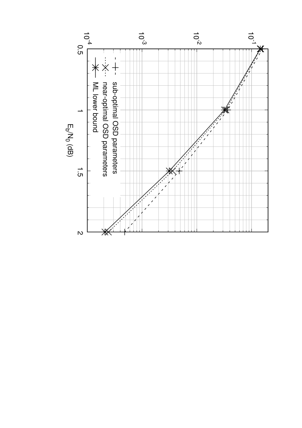
After having implemented these improvements, we can no longer use the rule to determine the optimal OSD order. Furthermore, the parameters of the improvements also have to be set. To determine if the decoder performs (near-)optimally, we make use of an ML lower bound calculated during computer simulation. Whenever the decoder outputs an erroneous estimate of the originally transmitted information word, the Euclidean distance between the original codeword and the received vector is evaluated. If this distance is larger than the distance between the decoder output and , then the ML decoder would also have made an erroneous decision.
Figure 1 shows the simulated performance of the (256,115) extended BCH code for two different choices of OSD parameters. The ML lower bound derived from the simulation with near-optimal parameters is also shown. We conclude that the second set of parameters leads to near-optimal results for this particular code at these signal-to-noise (SNR) values. The sub-optimal parameters, not considered in Section V, are however suitable for some practical applications because they lead to a decoding with a noticeably lower complexity at the expense of only a small loss of performance.
IV List of Codes suited to Short-Length Error-Correction
We apologize for not considering convolutional codes and turbo codes (parallel concatenated conv. codes) [20], [21]. Results on turbo codes will be included in a future work.
Given the recent research activity in the Coding community [22, 24, 25, 26, 27], we had to consider Polar codes and Reed-Muller codes. Also, BCH codes are known to be good codes at short length [2], [3]. Finally, LDPC codes from modern coding theory [4] are included. The list of binary codes regarded for performance comparison in the next section is:
- •
Reed-Muller codes: The code length is . Take Arikan’s kernel [22] and build its Kronecker product times, i.e. build . Then, select the rows of largest Hamming weight to get the generator matrix.
- •
Polar codes: As for Reed-Muller codes, rows are selected from . These rows correspond to highest mutual information channels after splittings. The generator matrix of the Polar code is found by exact splitting and adapted to each value of the channel parameter. For the BI-AWGN channel, we used density evolution [4] to split the channel and construct the code [23].
- •
- •
LDPC codes: Regular (3,6) low-density parity-check codes are built from a random bipartite Tanner graph [4]. Length-2 cycles are avoided, the number of length-4 cycles is reduced, but no other constraint was applied to the graph construction.
The use of a cyclic redundancy check (CRC) code to improve list decoding of polar codes was introduced by I. Tal and A. Vardy [24]. Here, given the universal nature of Gaussian elimination for ML decoding on the BEC and the universal nature of OSD decoding on the BI-AWGN channel, the CRC code was jointly decoded with all of the codes listed above to investigate its influence on the performance. By jointly we mean that a unique generator matrix is used for decoding. This joint matrix is simply the product of the CRC matrix with the generator matrix of the original code . Let be the generator matrix of . Let be the generator matrix of the CRC code, where is the degree of the CRC polynomial. Then, joint OSD decoding is based on the following generator matrix:
The serial concatenation has the CRC as outer code and the original error-correcting code as inner code. It is clear that the CRC will scramble the original matrix making any code look like a random code. We considered redundancy bits and the CRC-CCITT code with generator polynomial
V Performance Results
We ran computer simulations to obtain the performance of binary codes listed in the previous section. Randomly generated data is transmitted using the systems described in sections II and III. At every considered value of for the BEC and for the BI-AWGN channel, codewords were generated, transmitted, and decoded until 100 word errors occurred. During the computer simulation on the BI-AWGN channel, the ML lower bound was also recorded but we omit it from the figures to keep the graphs as clear as possible. The OSD parameters were chosen such that the performance is near-ML and the ML lower bound (almost) coincides with the actual simulated performance of the code.
Lower bounds on the optimal performance of finite-length codes exist for both the BEC and BI-AWGN channel. On the figures we include for the BEC the Polyanskiy-Poor-Verdú (PPV) bound on the maximal achievable rate, from Theorem 53 in [6],
where is the word error probability at coding rate , length , and BEC parameter . is the Gaussian-tail function. Computer simulations below take and or close to . On the BI-AWGN channel, we include the word error probability of optimal spherical codes, by C.E. Shannon [5],
where . The cone half-angle is computed by solving
The two above approximations from [5] are extremely accurate for lengths .
Figure 2 shows the word error rate versus the channel erasure probability for LDPC, Polar, RM, and BCH codes, all under ML decoding on the BEC. The performance of the LDPC code under iterative belief-propagation (BP) decoding is also included. No CRC is used for this performance comparison. The binary (256,131) BCH code is outperforming all other codes. Notice that the regular-(3,6) binary LDPC code has an excellent behavior.
Figure 3 shows the same codes on the BEC concatenated with the 16-bit CRC code given in Section IV. The horizontal scale in Figure 3 is from 0.44 to 0.5 only! All codes exhibit a performance within a small range of error rate. As mentioned in Section IV, the CRC scrambles the original generator matrix and the universal decoder (Gaussian elimination or OSD) does a joint decoding of both codes.
It is worth mentioning that the BCH code has dimension , hence its coding rate is higher than other codes and its PPV bound moves up with respect to the PPV bound at rate . This explains why the BCH code appears to be weaker, in fact it is closer to its PPV bound than the other codes.
The word error rate on the binary-input Gaussian channel is plotted on Figures 4 and 5, without and with CRC respectively. Figure 4 also includes the LDPC code under iterative belief-propagation (BP) decoding. With or without CRC, the (256,128) BCH code has the best performance versus the signal-to-noise ratio. As on the BEC, the CRC makes all codes behave almost like random codes, so the SNR gap between the worst and the best codes is very small.


VI Conclusions
We have compared the performance of four different short-length linear binary codes on the binary erasure channel (BEC) and the binary-input Gaussian (BI-AWGN) channel. The word error rate versus the channel parameter was plotted for LDPC, Reed-Muller, Polar, and BCH codes. In both channel scenarios, a universal, optimalnear-optimal decoder was used: the ML decoder for the BEC (via Gaussian elimination) and the OSD soft-decision decoder for the AWGN channel. From the computer simulation results, we conclude that the BCH code outperforms Reed-Muller, Polar, and LDPC codes on both channels. This behavior changes when we concatenate codes with a 16-bit CRC and perform joint decoding. As a result, the performance curves of the different codes lie much closer together and the choice of a good error-correcting code is not so critical.
Acknowledgment
Johannes Van Wonterghem would like to thank the Research Foundation in Flanders (FWO) for funding his PhD fellowship.
The work of Joseph J. Boutros was supported by the Qatar National Research Fund (QNRF),
a member of Qatar Foundation, under NPRP project 6-784-2-329.
The authors are grateful to Yury Polyanskiy for his precious and constructive comments on this work.
References
- [1] T.M. Cover and J.A. Thomas, Elements of Information Theory, Wiley-Interscience, 2006.
- [2] F.J. MacWilliams and N.J.A. Sloane, The theory of error-correcting codes, North-Holland, 1977.
- [3] R.E. Blahut, Algebraic codes for data transmission, Cambridge University Press, 2003.
- [4] T.J. Richardson and R.L. Urbanke, Modern coding theory, Cambridge University Press, 2008.
- [5] C.E. Shannon,”Probability of error for optimal codes in a Gaussian channel,” Bell System Technical Journal, vol. 38, no. 3, pp. 611-656, May 1959.
- [6] Y. Polyanskiy, H.V. Poor, and S. Verdú, “Channel coding rate in the finite blocklength regime,” IEEE Trans. Inf. Theory, vol. 56, no. 5, pp. 2307-2359, May 2010.
- [7] E. Arıkan, “Channel polarization: A method for constructing capacity achieving codes for symmetric binary-input memoryless channels,” IEEE Trans. Inf. Theory, vol. 55, no. 7, pp. 3051-3073, July 2009.
- [8] S. Kudekar, T. Richardson, and R.L. Urbanke, “Spatially coupled ensembles universally achieve capacity under belief propagation,” IEEE Trans. Inf. Theory, vol. 59, no. 12, pp. 7761-7813, Dec. 2013.
- [9] W.E. Ryan and S. Lin, Channel Codes, Classical and Modern, Cambridge University Press, 2009.
- [10] B. Dorsch, “A decoding algorithm for binary block codes and J-ary output channels,” IEEE Trans. Inf. Theory, vol. 20, pp. 391-394, May 1974.
- [11] J. Fang, “Décodage pondéré optimal des codes linéaires en blocs et quelques sujets sur la complexité du décodage”, PhD Thesis, ENST, March 1987
- [12] M. P. C. Fossorier and S. Lin, “Soft-decision decoding of linear block codes based on ordered statistics,” IEEE Trans. Inf. Theory, vol. 41, no. 5, pp. 1379-1396, Sep. 1995.
- [13] M. Fossorier, “Reliability-based soft-decision decoding with iterative information set reduction,” IEEE Trans. Inf. Theory, vol. 48, pp. 3101-3106, Dec. 2002.
- [14] A. Valembois and M. P. C. Fossorier, “Box and match techniques applied to soft-decision decoding,” IEEE Trans. Inf. Theory, vol. 50, no. 5, pp. 796-810, Dec. 2004.
- [15] W. Jin and M. P. C. Fossorier, “Probabilistic Sufficient Conditions on Optimality for Reliability Based Decoding of Linear Block Codes,” IEEE International Symposium on Information Theory, Seattle, WA, pp. 2235-2239, 2006.
- [16] Y. Wu and C.N. Hadjicostis, “Soft-Decision Decoding of Linear Block Codes Using Preprocessing and Diversification,” IEEE Trans. Inf. Theory, vol. 53, no. 1, pp. 378-393, Jan. 2007.
- [17] Y. Wu and C.N. Hadjicostis, “Soft-Decision Decoding Using Ordered Recodings on the Most Reliable Basis,” IEEE Trans. Inf. Theory, vol. 53, no. 2, pp. 829-836, Feb. 2007.
- [18] W. Jin and M. P. C. Fossorier, “Reliability-Based Soft-Decision Decoding With Multiple Biases,” IEEE Trans. Inf. Theory, vol. 53, no. 1, pp. 105-120, Jan. 2007.
- [19] Y. Wu and M. P. C. Fossorier, “Soft-decision decoding using time and memory diversification,” IEEE International Symposium on Information Theory, Toronto, ON, 2008, pp. 76-80, 2008.
- [20] C. Berrou and A. Glavieux, “Near optimum error correcting coding and decoding: Turbo-codes,” IEEE Trans. on Communications, vol. 44, pp. 1261-1271, Oct. 1996.
- [21] S. Benedetto and G. Montorsi, “Unveiling turbo-codes: some results on parallel concatenated coding schemes,” IEEE Trans. on Inf. Theory, vol. 42, no. 2, pp. 409-428, March 1996.
- [22] E. Arıkan, “A performance comparison of polar codes and Reed-Muller codes,” IEEE Comm. Letters, vol. 12, pp. 447-449, June 2008.
- [23] R. Mori and T. Tanaka, “ Performance of polar codes with the construction using density evolution,” IEEE Comm. Letters, vol. 13, pp. 519-521, July 2009.
- [24] I. Tal and A. Vardy, “List decoding of polar codes,” IEEE International Symposium on Information Theory, St. Petersburg, Russia, pp. 1-5, 2011.
- [25] M. Mondelli, S.H. Hassani, and R. Urbanke, “From Polar to Reed-Muller Codes: a technique to improve the finite-length performance,” arXiv:1401.3127 [cs.IT], Sept. 2014.
- [26] H. Vangala, E. Viterbo, and Y. Hong, “A Comparative Study of Polar Code Constructions for the AWGN Channel,” arXiv:1501.02473 [cs.IT], Jan. 2015.
- [27] S. Kudekar, S. Kumar, M. Mondelli, H.D. Pfister, E. Sasoglu, and R. Urbanke, “Reed-Muller Codes Achieve Capacity on Erasure Channels,” arXiv:1601.04689 [cs.IT], Jan 2016.