On the Tree-Like Structure of Rings in Dense Solutions
D. Michieletto,a
Received Xth XXXXXXXXXX 20XX, Accepted Xth XXXXXXXXX 20XX
First published on the web Xth XXXXXXXXXX 200X
DOI: 10.1039/b000000x
One of the most challenging problems in polymer physics is providing a theoretical description for the behaviour of rings in dense solutions and melts. Although it is nowadays well established that the overall size of a ring in these conditions scales like that of a collapsed globule, there is compelling evidence that rings may exhibit ramified and tree-like conformations. In this work I show how to characterise these local tree-like structures by measuring the local writhing of the rings’ segments and by identifying the patterns of intra-chain contacts. These quantities reveal two major topological structures: loops and terminal branches which strongly suggest that the strictly double-folded “lattice animal” picture for rings in the melt may be replaced by a more relaxed tree-like structure accommodating loops. In particular, I show that one can identify hierarchically looped structures whose degree increases linearly with the size of a ring, and that terminal branches are found to store about 30% of the whole ring mass, irrespectively of its length. Finally, I draw an analogy between rings in the melt and slip-linked chains, where contact points are enforced by mobile slip-links and for which a field-theoretic treatment can be employed to get some insight into their typical conformations. These findings are ultimately discussed in the light of recent works on the static structure of rings and on the existence of inter-ring threadings.
1 Introduction
††footnotetext: a School of Physics and Astronomy, University of Edinburgh, Peter Guthrie Tait Road, Edinburgh EH9 3FD, Scotland, United Kingdom.One of the last big mysteries in polymer physics is understanding the behaviour of rings in dense solutions and melts 1, 2, 3. Beyond the case of systems composed by synthetic ring polymers 3 which are of interest for the design of novel materials, there is a broad and general interest in understanding the organisation of bacterial genomes 4, 5 and kinetoplasts 6, 7, largely composed of closed (ring) DNA.
It is nowadays well accepted that, in the limit of large polymerisation index , rings in the melt assume configurations which display a typical size scaling as 8, 9, 10, 11 , with . This value of the metric exponent is usually associated with collapsed polymers in poor solvents, which tightly fold onto themselves expelling other chains and solvent from their interior volume. On the other hand, recent works 12, 13, 14, 15 pointed out that the fraction of a ring’s contour length that is in contact with any other ring in solution does not scale as , as the smooth surface of a compact sphere would, but rather as , indicating a very “rough” surface and a low degree of segregation. In agreement with this finding, several very recent works from different groups 12, 16, 17, 18 reported that rings in dense solutions display largely inter-penetrating configurations: segments of rings double-fold and thread through the contour of their neighbours, eventually leading to strongly overlapping configurations, perhaps best mimicked by the behaviour of ultra-soft colloids 19 rather than by that of polymers in poor solvents.
Another important element in the picture is that some decades ago it was discovered that ring polymers embedded in a fixed background of obstacles assume configurations known as “lattice animals” (LA) 20, 21, 22, 23, 11, 24, 25, 26, 27. These conformations have a characteristic double-folded shape which can branch into complicated and ramified “tree” structures. LAs are a natural consequence of the topological invariance of the system: rings which are prepared un-knotted and un-linked from any other ring or from the background of obstacles have to remain un-knotted and un-linked at any time. For a ring diffusing in a tight gel, i.e. with lattice spacing of the order of the ring’s persistence length, the entropy-maximising choice that satisfies these topological constraints is to double-fold onto itself and snake through the gel pores.
As argued in the literature 20, 28, 11, the situation of rings in the melt can be thought of as similar to the case of self-avoiding rings in an array of obstacles. In the ideal chain limit, field-theoretic arguments led a number of authors 24, 29, 20 to predict this system to be in the same universality class as ideal randomly branched polymers for which a metric exponent was found. Since this value of would lead to a divergence in the density of the system, some authors 20, 29 also suggested that the polymer would attain the lowest physically possible value of , or in 3D. The self-avoiding limit of the same system (randomly branched polymers) was instead shown 30 to display in 3D.
Numerical 8, 13, 12 and experimental 31 evidence seem to suggest that the self-avoiding regime () in fact holds only for short rings, whereas the ideal behaviour () takes over in the limit of large polymerisation index through a broad crossover where 22 . These arguments seem to lead to a picture of “crumpled lattice animals” where globally collapsed polymers display local tree-like structures.
While the global structure of the rings can be directly inferred from the metric exponent in simulations 10, 12 (or neutron scattering in experiments 31), their local structure is more difficult to probe. Although the existence of local tree-like conformations has been conjectured, there is only circumstantial evidence for their existence in the literature. In this work, the aim is to explicitly prove and quantify the presence of branches and tree-like structure in the conformation of ring polymers in dense solutions.

In order to achieve this aim, one important step is to find a method able to identify branches and tree-like structures in the configurations of rings. Characterising their conformations is in fact an open challenge 11, 10, 13 and one of the most important contributions in this direction has been made in Ref. 10 where the authors elegantly showed (through numerical simulations) that equilibrated configurations of rings in solution displayed very little change with respect to their initial state when prepared as densely packed lattice animals. In Ref. 10 the authors focus in particular on global observables, such as the gyration radius of the rings. Here, I will be using the data obtained from large-scale Brownian Dynamics simulations of rings in dense solutions (from Ref. 12) to identify tree-like structures at the local scale of the rings’ segments (see Fig. 1 for a snapshot of the system and Appendix A for details on the Brownian Dynamics simulations).
I will show that quantitative insight can be achieved by looking at instantaneous maps of the contacts between sections of the rings: characteristic contact patterns in fact seem to emerge, and from these, one can identify tree-like structures. By computing the writhing of rings’ segments, I will show that it is possible to get an accurate measure of the number and typical length of the terminal branches. Moreover, isolated spots in the contact map are shown to reveal the presence of loops which can be long-ranged, i.e. of order . The hierarchical looping of these structures is then addressed and from there, an analogy to a system of slip-linked rings is drawn. By making use of the field theoretic treatment developed by Duplantier 32 for networks of polymers, I finally discuss possible insights that can be obtained by further extending the analogy with slip-linked chains.
The results presented in this work can be used to gain a deeper understanding about the general behaviour of rings in dense solutions and in particular about the existence of tree-like structures at the local scales. They may also be used to obtain further insight into the probability of inter-penetration between rings 12, 18 and may complement recent findings on the statistics of threadings’ lengths and how these depend on the rings’ total contour length 16. These unresolved issues in fact seem to play a crucial role in some of the unexplained features displayed by rings in the melt, such as their very prolonged sub-diffusive regime 14 – which extends much further than the typical length-scale observed for linear polymers – or the “fat-tails” displayed by the stress-relaxation function 14, 3, 33, which seem to capture some unexpected long-time collective behaviours of the rings.

2 Patterns in the Contact Maps Reveal Loops and Branches
The first part of this work is aimed at achieving a basic understanding of how one should tackle the problem of characterising tree-like structures and what are the main observables to use. One of the most useful quantities is the instantaneous contact map, or matrix, of a configuration. Such a map is generated by recording the contacts between the segments (beads) making the polymer contour. In particular here I will set the entries of the contact matrix as
| (1) |
where if and 0 otherwise and is the threshold chosen to determine that two beads are “in contact” ( is the nominal size of a bead and throughout this work). These matrices are broadly used in biophysical experiments to determine the 3D organisation of genetic material of eukaryotes 34, 35, 36, 37, 38 and bacteria 4, 39. As in the case presented here, although on a much more complex level, characteristic patterns seem to emerge 35, and their understanding is one of the major challenges in the field of biophysics.
In Fig. 2(A-B) I give some examples of contact patterns that one can observe in idealised and naive tree-like conformations compared to a real contact map computed from the conformation of a ring polymer in dense solution. It is useful to bear in mind that contact maps are symmetric with respect to the operation (as one can see from eq. (1)). This means that recording the upper or lower half of the matrix is enough to fully characterise the contacts. For this reason in Fig. 2 I only report the upper of lower triangle of a contact map.
From the figure one can readily notice that perfectly double folded rings, or lattice animals, have characteristic contact patterns. The first feature is the main diagonal which comprises the points
| (2) |
and captures the beads self-interaction and the chain connectivity. Second, trunks, or backbones (see for instance and in Fig. 2(Aii)), are elements of the set of lines of length
| (3) |
where represents an arbitrary translation along and a modulo operation is taken implicitly due to the periodicity of the beads indexes introduced by the ring closed topology.
This symmetry entails the existence of a family of contact maps which all capture the same LA conformation and it is also interesting to notice that thanks to the composition of the two symmetries of the system, i.e. and one can readily identify points along the contact map boundaries so that . For instance, points bi1 and bi2 in Fig. 2(Ai) can be identified as the same point, this would not be possible if the polymer was linear (see also Appendix B).
The last element to point out is the set of “terminal branches” (see in Fig. 2(Ai)-(Aii)), also sometimes called “leaves”, which belong to a subset of determined by the fact that the elements of this set have to originate from , i.e.
| (4) |
At this point it is worth reminding that Figs. 2(Ai)-(Aii) represent idealised and perfectly double folded LA configurations. In reality, rings in dense solutions would hardly look exactly like these. By relaxing the constraint on the double-folded structure, one can draw LA-like conformations which can accommodate loops (see inset of Fig. 2(Bi)). Loops are represented as “spots” in the contact maps and they can be classified as elements of a subset of where , i.e. including short segments.
Finally, Figure 2(Bii) reports the contact map obtained from a ring beads long equilibrated in a dense solution (from Ref. 12). In this case the contact map shows the presence of some structures which can be associated to those of idealised LA, such as terminal branches, but it also shows the absence of long trunks at the advantage of several spots, or loops, which assume hierarchical, i.e. “loop-within-loop”, character. For instance loops L1,L2 and L3 in Fig. 2(Bii) form a “higher order” looped structure that is also commonly known as a “rosette” 40, 41 or “transitive” loops 35. This type of looped structure has been identified in the contact maps obtained from “Hi-C” 35 experiments on eukaryotic nuclei and it has been associated with the presence of transcription factories 42, 43 and with other types of ATP-driven organisation of chromosomal domains in both, interphase and metaphase chromosomes 44, 45, 46, 35, 47. It is somewhat intriguing to find similar patterns in the much simpler case of a dense solution of ring polymers as the one studied in this work; in particular, it may suggest that these higher-order looped architectures may also be guided by entropic forces working alongside topological constraints (more on this in the next sections).
The final remark I would like to make in this first Section is that the contact map shown in Fig. 2(Bii) displays some patterns (circled in red) that are more difficult to interpret uniquely at this stage. These in fact might capture either terminal branches or loops. In order to better classify these patterns one may want to seek for other observables: in the next section I will show that one possible choice is the local unsigned writhing of the polymer segments.
3 Local Writhing Identifies the Location and Length of Terminal Branches
One of the main motivations for introducing the “writhe” of a curve some decades ago 48 was to describe the super-coiling of torsionally constrained (closed) elastic ribbons such as circular double-stranded DNA 49. In this case, the writhe of the ribbon (Wr) is connected to the linking of its two edges (Lk) and its twist (Tw) via the formula 48, 49.
In fact, by taking the limit of infinitely narrow ribbons, it is possible to generalise the writhe of a ribbon to a single curve and directly compute its writhing number as the Gauss integral 49, 50, 51
| (5) |
This quantity can be thought of as the result of (i) summing the (directional) self-crossings of the curve associated with a particular two-dimensional projection and of (ii) averaging over infinitely many viewpoints 51. In other words it is a measure of how much entangled the curve is with itself.
The writhe of curves and polygons has been studied in the past as a measure of their entanglement in a number of works (see e.g. Refs. 52, 53, 54, 55, 56 and references therein). In the large majority of these works the authors have investigated the global writhe of polymers, either free 52, 53, in confinement 56 or in dense and poor solutions 52.

In the case of achiral polymers it is also useful to consider a variant of eq. (5) which better captures the degree of self-entanglement of a torsionally relaxed curve. This quantity is obtained by removing the information on the directionality of the crossings and it is therefore defined as the “unsigned” writhe, or “average crossing number”57, 58, 59:
| (6) |
Eq.(6) gives a measure of the average number of crossings of the whole curve , or polymer configuration. In principle, one can generalise this quantity for the case of local polymer segments 60, 50 and, in particular, it is possible to define a “segmental average crossing number” or “local unsigned writhing” as
| (7) |
which gives a measure of the (un-directional) self-crossings of the segment .
In light of this generalisation, and in analogy with the findings for plectonemes in supercoiled DNA 50, it is natural to ask whether terminal branches display a higher value of with respect to a non-branched part of the polymer contour length. In practice, I employ the numerical scheme discussed in Ref. 50 to compute the profile along the contour of ring polymers made of discrete beads ranging from to using a fixed value of ** * Large values of result in flatter profiles which lose the ability of detecting short branches. On the other hand, segments can writhe only on length-scales larger than the Kuhn length . As discussed in Appendix C, the optimal value for seems therefore to lie in between 1 and 2 Kuhn lengths..
In Fig. 3 I report an example of the profiles obtained using this procedure on the same ring that yields the contact map shown in Fig. 2(Bii). The figure shows as well as the 2D projection used in Fig. 2(Bii) this time colour-coded in terms of the value attained by the local unsigned writhe. One can readily notice the presence of three peaks which correspond to the two branches already identified in the contact map (B1 and B2 in Fig. 2(Bii)) and a third, which could have been classified as a loop near the main diagonal (middle branch). It is therefore natural to identify the location of terminal branches with the local maxima of the function . Furthermore, it is also possible to determine the length of the terminal branches by measuring the distance between the first two local minima at the sides of each peak (in practice one also requires that the value of the local unsigned writhe is above (below) a certain threshold () in order to remove spurious fluctuations, see also Appendix C).

3.1 Statistics of Branching
At this point it is natural to ask several questions regarding the nature of the terminal branches, for instance how does their statistics vary with the length of the rings?
As reported in Fig. 4(A), the number of terminal branches per ring, , is normally distributed (solid lines represent Gaussian fits) and the mean increases linearly with the ring size, (shown in the inset). This finding is interesting when seen in light of the fact that the number of inter-penetrations between rings was also found to scale linearly 18, 16 with the ring size. It may therefore be tempting to associate threadings with at least some of the terminal branches.
While the number of branches grows with the length of the rings, their average length, , is instead observed to robustly attain the value of beads independently of (see inset Fig. 4(B)). Importantly, the fact that is independent of the total ring length is valid for any choice of the parameter (see Appendix C) and it is in full agreement with the observation that the bond auto-correlation function measured for rings in dense solutions displays a negative dip whose minimum is located at few persistence lengths irrespectively of the total ring length 61, 62, 10. On the other hand, this finding does not exclude that there might be hierarchical branches whose effective length extends further than ; the algorithm proposed in this section only captures terminal branches, and does not quantify higher order structures such as branches within loops, for instance. A further remark is that the distribution of lengths shown in Fig. 4(B) is not simply Gaussian, as in the case of but it displays “heavy tails” and it may be better fitted by a log-normal distribution. In other words, some of the branches extend much further than the average length .
Because and it follows that the number of beads involved in terminal branches must also scale with . This is shown in Fig. 4(C) where I report that the probability distribution of observing a certain fraction of contour length inside terminal branches. As one can readily notice, the distribution narrows when longer rings are considered while its mean, (shown in the inset), appears to be independent on and it amounts to about the 30% of the total ring’s mass.
From the results reported in Fig. 4, it is straightforward to extract also the free energy associated with generating branches on a ring beads long as
| (8) |
where is the mean value of the fitted , and its variance.
From eq. (8) one can notice that the free energy penalty involved in creating one additional branch from an equilibrium state decreases with and it is about for a 25 beads segment. This free energy difference comes from the competition between the bending energy cost and the entropy gain of forming an extra branch. The former term can be crudely computed as the energy required to bend an elastic rod of length and persistence length into an “O” shape (see regions of high local writhe in Fig. 3(A)), i.e.
| (9) |
while the resulting entropic gain is .
The numbers that can be extracted from Fig. 4 and eq. (8) also allow one to estimate that the free energy minimising configurations possess one terminal branch, on average, every 90 beads and, by using the fact that its average length is about 25 beads, one can also estimate the average separation between branches as being about 65 beads.
In light of this and of the fact that for it may be tempting to conjecture a possible mechanism able to robustly select a typical branch length: (i) very short branches are energetically very costly (see eq. (9)) therefore (ii) branches sprout only when capable of covering a certain contour length (see Fig. 4(B)); starting from these ‘‘sprouts’’, terminal branches keep growing proportionally to their length (and hence the multiplicative ‘‘heavy tails’’ displayed by the distribution of lengths) until a critical length of around 50-65 beads is reached†† † The precise numbers will be, of course, system dependent, while the general mechanism should be more general.. At this point they split into further terminal branches while the part of the original branch moves away from the main diagonal in the contact map, i.e. from the set to , and only the remaining tips are identified as terminal branches. This is because only the terminal branches remain tight and highly self-entangled while the branches that move away from the diagonal open up to become “loose” (more about this mechanism is discussed Section 5 through the analogy with slip-links).
Finally, it is worth highlighting the finding that the fraction of contour length that is stored in the terminal branches for any one ring is, on average, the 30% of its whole mass ‡‡ ‡ For comparison, some species of biological trees seem to display a “leaf mass ratio” in the range 63 25-35% while others (Acacia or Acer) reach a staggering 64 50-60%. (see inset Fig. 4(C)). One should in fact bear in mind that the branches captured by the algorithm discussed in this section are only the terminal ones, i.e. no higher order branching is identified and quantified at this stage. In the next Section I will attempt to characterise the higher levels of organisation of the rings by quantifying their hierarchical looping.

4 Hierarchical Looping
An interesting observation that was pointed out in Refs. 28, 11 and discussed in Sec. 2 is that rings in the melt do not need to display a strictly double-folded structure; in fact, they can accommodate loops. The presence of loose loops in the configurations of ring polymers in the melt was first identified in Ref. 13 (where they were also referred to as “voids”) and it can be readily observed in the snapshot reported in Fig. 1 or in the contact map plotted Fig. 2, where the spots are scattered and do not form long lines as for the case of idealised LA. It is also tempting to associate loose loops with openings of the double-folded structure which offer some “threadable” surface 16 to the neighbouring rings. For this reason it may be of interest to quantify the number of loops, their typical size, and some of the hierarchical structures that may emerge when multiple loops come together.
From a contact map such that the one showed in Fig. 2(Bii) it is possible to extract the number of isolated spots. The general procedure requires two steps: (i) marking the boundaries of the spots by checking the presence of clustered “on” pixels against the “off” background, and (ii) enumerate different clusters by progressively adding the boundary points that fall within a certain radius of one-another. Here I set since one may argue that contacts between beads that are shorter than two persistence lengths cannot form ‘‘loose’’ loops since the connecting segments are stiff on this length scale§§ § Again, one may argue that in the limit one loses information of the fine looped structure, while in the other limit small chain fluctuations may lead to “false” isolated spots. The scaling properties of the derived observables and the general picture should not be affected by the precise value of in the range of few persistence lengths..
Furthermore, one can use the knowledge of the length of the terminal branches (extracted from Fig. 4) to exclude spots which are closer than to the main diagonal, where is defined through the following formula
| (10) |
and in order to exclude the large majority of terminal branches that may appear as spots in the contact map (the results reported are not sensitive to the precise value of as long as it allows one to discriminate between a loop and a terminal branch).
Following this procedure one obtains contact maps with enumerated spots as exemplified in Fig. 5(A) where I report the same contact map shown in Figs. 2(Bii) and 3, but where the boundaries of isolated spots are now marked in different colours and enumerated.

4.1 Statistics of Looping
One of the quantities that can be easily extracted from this procedure is the number of loops, , as a function of the rings size; the distribution and the (roughly linear) scaling of the mean value is shown in Fig. 5(B). A further interesting observable to quantify is the size of the loops. The probability of observing a loop of size is clearly related to the probability of contact between two segments distant beads apart, , often investigated in relation to the statistics of rings 11, 12 and to obtain information on the 3D configuration of bio-polymers 65, 35, 41. This probability is known to scale as
| (11) |
with a “contact” exponent 11 and one may expect to scale with the same exponent.
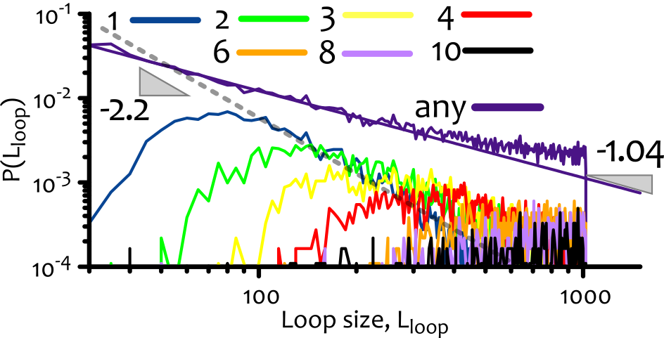
In order to extract this distribution from the contact map one can consider the geometric centre of the spots computed from their boundaries (see Fig. 5(A)) and measure the loop size from its location as , which accounts for periodic boundary conditions in the rings indexes (in practice, I also require to be smaller than again for symmetry considerations and the constraint on the length of the terminal branches). The number of observations of a loop of length across the sampled rings is then normalised by the total number of loops to give the probability distribution shown in Fig. 6. In agreement with the previous argument, is found to decay as a power law with an exponent compatible with the known values of and in particular with the one directly measured (in Ref. 12) on the configurations of the rings studied in this work ().
A direct consequence of this scaling is that loops can be formed at any length-scale, i.e. there is no preferred loop size, differently from the case of terminal branches where a selected length-scale could be observed. A further interesting point is that the curves in Fig. 6 display a “bump” in the region which may suggest a number of loops covering order contour length above the one predicted by scaling (the same “bump” was already observed in Ref. 13 through the contact probability ).
4.2 Hierarchy of Looping and Looping Degree
The last aspect of looping which is left to address is its hierarchical architecture. For instance, loops 7,6 and 5 in Fig. 5 may be thought of as progressively forming “loops within loops”. Another example also previously discussed is the case of “rosettes” 40 where multiple loops come together in a single 3D hub such as the one formed by loops 2,3,4 and 5 in Fig. 5 (see also Fig. 2); these have also been recently called “transitive loops” in the specific case of the organisation of the so-called “topologically associated domains” 35.
In order to quantify these hierarchical structures one can recursively classify the loop degree of spots which contain other spots (always excluding the spot in the corner (0,M-1) and in practice allowing some degree of error in the location of each spot), and assign the highest score of “looping degree”, , to the whole tree-like structure. For example, loops near the terminal branches (such as “7” or “2” in Fig. 5) would score a loop degree while loop “3” would have ¶¶ ¶ It is interesting to mention that one can use this classification of the loops to re-analyse the distribution of loop sizes for each looping degree. The results of this analysis are reported and discussed in Appendix D and in Section 5.. The result of this algorithm is sketched in Fig. 7(A) where the same contact map of Fig. 5(A) is shown (turned by 45∘). The spots are this time labelled as L1-L6 and coloured in terms of their looping level.

From this figure it is interesting to notice that there are two clear types of structures in the same tree: the first is a “rosette” formed by loops L1-L4, i.e. these four loops come together in the same 3D “hub”; this can be readily identified by the fact that part of their “boundaries” are shared, which means that the beads at the base of the loops are near one another in 1D, and therefore, also in 3D. The second structure is made by loops L4-L6 which form “loops-within-loops” in a fashion that resembles a stapled hairpin, or a “stack” – i.e. an aligned cluster – of slip-links 66 (also called a “necklace”). This structure is rather different than a rosette which can instead be pictured, by extending the analogy, as an isotropic cluster of slip-links. It is also worth mentioning that a “rosette” implies only the 3D co-localisation of the contact points forming loops, and does not specify any topological information about the cluster of loops. On the other hand, the “necklace” has a specific topological structure (more on this later).
Finally, an interesting quantity that can be extracted from the described procedure is the looping degree of a given tree-like structure. In Fig. 7(B), I report the distribution of this quantity, which can give an estimation of the number of hierarchical levels in the tree-like representation of a ring. Interestingly, the mean of the distributions is found to scale linearly (within errors) with the size of the rings (see inset).
Summarising, in this section I have shown that the configurations of ring polymers (captured through their contact maps) display loops, which strongly suggest the absence of a perfectly (or even partially) double-folded LA conformation. Furthermore, loops can have a hierarchical structure, and the degree of the hierarchy scales linearly with the size of the rings. Loops in the conformation of rings can be thought of as temporary contacts, and one important consequence of the findings reported in this section (Fig. 5) is that the number of loops tends to fluctuate around . A crude approximation of such a picture is that of a ring with a fixed number of contact points which can diffuse along the ring contour. In turn, this approximation is extremely akin to that of a ring decorated with slip-links. This analogy (which was introduced earlier to describe the two topological structures observed previously) will be further explored in the next section.
5 Analogy with Slip-Linked Rings
A ring configuration is the result of the competition between energetic and entropic forces, the former favouring the presence of few large loops, the latter favouring the creation of many short terminal branches. In order to shed some light on the possible structures that such interplay might produce it may be of help to push the analogy with slip-linked chains mentioned earlier further.
As briefly introduced in the previous section, the findings reported in Fig. 5 support a (crude) approximation where a ring polymer embedded in dense solution or melt can be thought of as a slip-linked chain with slip-links. These can freely diffuse along the polymer contour and enforce the presence of contact points while also allowing the exchange of contour length among the ring segments stored in between the slip-links.

To put this analogy more in the context of rings in the melt, one may imagine that the entanglements and topological constraints experienced by the rings in dense solutions form effective tight “gates” 28 which “squeeze” some parts of a given ring polymer. Because of the rings closed topology, such a gate would enforce a sliding contact point for the polymer segments as long as the entanglement is present. For this reason, while physical slip-links are only allowed to slide along the chain, in this case it may be more appropriate to envisage a combination of sliding and un-binding/re-binding with a typical rate that is related to the entanglement relaxation time.
It might also be worth pointing out at this stage that within this model slip-links would be allowed to form pseudo-knots. Although barely noticeable in the contact map in Fig. 7(A), a close inspection of the 3D configuration of the ring (see Suppl. Movie M1) reveals that loops L2-L1 and L4-L3-L1 cross each other. In other words, the arc diagrammatic representation 66 derived from the contact map (Fig. 8(A)) contains crossing arcs. In addition, it is worth highlighting that loops L1-L4 still form a rosette in 3D, but now the topology of the rosette (unknown before) is also determined. ∥∥ ∥ The abundance of pseudo-knotted configurations can be readily measured by checking for loops which stem from base-points that alternate along the contour of the ring. Pseudo-knots appear in about 50% of the configurations for , 85% for and more than 99% for .
5.1 Theory for Slip-Linked Chains
The slip-links analogy naturally lends itself to be discussed in terms of these arc-diagrammatic representations. For instance, the contact map in Fig. 7(A) can be represented as the arc-diagram shown in Fig. 8(A). Fig. 8(B) shows the diagram in terms of a ring configuration with physical slip-links while Fig. 8(C) shows the corresponding “polymer network” representation 32, 66.
Borrowing from the work of Duplantier 32, there are several observations that can be made solely based on the topology of the network representation. In general, the number of configurations for a polymer network made by chains with lengths summing up to and joined at vertexes of functionality is given by
| (12) |
where is an appropriate scaling function and is a topology-dependent exponent equal to
| (13) |
In eq. (13) is the number of closed paths**** ** Closed paths in the network represenation of a slip-linked chain are also incidentally called “loops”. These are different from the loops discussed in the previous sections, whose size was defined as the whole stretch of contour length separating two monomers near one another in 3D space. Here, the size of a closed path is the sum of the segments joining vertexes in the network representation. in the graph, the number of vertexes of functionality and the exponent related to the -leg vertex 32.
It is also worth noticing that slip-links locally appear always as a 4-legged vertex. This implies that the exponent can be computed directly by knowing only the number of slip-links on the chain. In the case of slip-links one has
| (14) |
In turn, this entails that the exponent of a ring polymer with fixed number of contacts remains the same, no matter the specific global topology of the network. For this reason, the simpler network represented in Fig. 8(D) obtained by shifting the arcs L2 and L4 inside the arcs L1 and L3-L1 respectively, has the same exponent as the graph in Fig. 8(C) (this argument of course neglects the scaling function which can instead vary 66, 67).
In terms of the jargon introduced in Ref. 66, the network shown in Fig. 8(D) is a ‘‘round-table’’ (small loops decorating a large central loop made by L1,L2 and L3†††† †† It is worth reminding that due to the ring periodicity, loop L1 can be seen as non-containing L2 and L3, i.e. these three loops do not form concentric arcs.), glued to a “necklace” (concentric arcs made by loops L4-L6). Further physical properties of these two special topologies can be inferred 66 from eq. (12); in particular, one can obtain informations about the statistics of loop sizes and this, in turn, might shed some light into the findings of the previous sections and, in general, on the configurations of ring polymers in the melt.
Starting from the assumption that all the decorating loops are small compared to the central one, the “round-table” configuration with closed loops connecting the vertexes carries a statistical weight (see also Fig. 8(E))
| (15) |
This means that while the central loop is swollen () due to the sliding entropy of the slip links, the decorating loops are tight () therefore being self-consistent with the initial assumption. For the “necklace” structure one in general finds that the terminal loops are expected to be tight, as one would expect for terminal branches, while one of the inner loops can be swollen, i.e. of the size of the whole contour length.
5.2 Applications of Slip-Link Theory to Rings
Understanding how the statistics of loop lengths changes when the “round-table” and the “necklace” structures are glued together or in the case of more complex network topologies such as the one in Fig. 8(C) is far from the scope of this work and it remains an open challenge for the future. Nonetheless, it is interesting to notice that the distribution of loop sizes for loops of degree zero – i.e. the smallest ones that appear in the contact map and that do not contain any other loop – shows a power law decay with an exponent remarkably close to the value predicted by the field theory for the size of tight loops on slip-linked chains (see Fig. 9 and Appendix D). This might suggest that the smallest loops appearing in the conformations of rings might indeed be thought of as originating from a slip-link model.

Another interesting remark that may be relevant for completing the analogy between rings in the melt and slip-linked chains is that it would be of interest to compare the behaviour of rings in dense solutions with that of rings with “sticky” slip-links. This model would in fact display a transition between a swollen coil and a collapsed globule with branches sticking out – a sort of sea urchin or large rosette – depending on the interaction strength.
Crudely, the transition point may be inferred from the free energy of slip-links interacting with attraction energy and forming loops of equal size . By making use of eq. (14) one may write
| (16) |
where the first term increases only linearly in in the limit of a large rosette due to the finite number of interactions that any one slip-link can make with its neighbours. The last term in eq. (16) can be obtained from eq. (12) in the limit where all loops have equal size and the rosette is made by slip-links (vertexes) having 4 legs each. The system with the free energy expressed in eq. (16) displays a transition between the fully swollen state and the fully collapsed “sea-urchin” state, the latter being attained for
| (17) |
By using for , , and considering loops made by 50 beads and a number of 10 maximum number of neighbours per each slip-link () one obtains a critical attraction strength of .
In addition to this crude estimation, it may be relevant to study (i) a more accurate model where slip-links are allowed to move along the chain and can form loops of different sizes and (ii) an effective non-equilibrium model where the binding/un-binding kinetics of the slip-links – related to the temporary nature of the entanglements with the neighbours – may affect the steady state of the system. By drawing an analogy to the recent work on “ephemeral” DNA-binding proteins 68, the (un)binding kinetics may, also in this case, offer a mechanism through which the coarsening towards a large rosette is arrested and the coexistence of several structures is stabilised. Finally, it would be interesting to investigate whether the structures produced by these models might resemble those assumed by rings in the melt.
6 Trees, Slip-Links and Threadings
One important message of the previous Section is that in the case of simple networks made of slip-linked chains, loops of completely different sizes have been shown to coexist (e.g. very tight and very loose in the round-table configuration). From the analogy with slip-linked chains it is therefore tempting to speculate that rings in the melt might also be able to show coexistence of long-ranged loops and small ones.
The presence of long-ranged and “loose” (in that they do not form a double-folded trunk) loops, although in contrast with the classical double-folded LA picture for rings in the melt, is supported by several findings: (i) large tails in the statistics of contacts 13 and of loop sizes (see Fig. 6) which indicates the significant presence of looping, (ii) the absence of strictly double-folded, or ideal lattice animal, conformations 13 and the observation of “voids” in the rings configurations 13 and (iii) the presence of threadings whose number grow with the length of the rings 18, 12 and with the size of their minimal surface 16. All these observations tend to suggest that rings display loose long-range looping which may lead to large “threadable” surfaces, not unlike certain equilibrium configurations of slip-linked rings 66.
This conjecture naturally leads also to the following speculation: a solution of dense ring polymers, obtained by squeezing together tight and loose loops from neighbouring chains, is bound to show the presence of threadings formed by tight loops accommodated inside the loose ones. The behaviour of these threadings may also be imagined (as argued in Ref. 16) as random walks originating and returning to planes formed by the locally flat minimal surface spanning a threaded ring. This argument is supported by the distribution of threading lengths which is shown to be well fitted by a power law with an of exponent compatible with that expected for a 3D random walk in between interactions with a surface.
6.1 Threadings as (non) Returning Walks
A relevant observation in regard to this conjecture is that the exponent can be observed for the distribution of lengths of 3D random walks that can be absorbed only by the origin (see Fig. 10(A)). In this case, though, the returning probability is smaller than one 69, and this in turn implies that some of the walks are never re-absorbed by the origin (and hence the spike at large walk lengths shown in Fig. 10(A)).

This observation may have some significance for estimating the length and extension of a threading. In fact, a threading displays, by definition, both an outgoing and an ingoing segments passing through the threaded chain. While the ingoing segment is bound to return to the threaded region, the outgoing segment can freely wander as if it was a truly free random walker in 3D. In other words, the tip of a threading may be thought of as the one performing a 3D random walk in space.
In the case the threading originates from a very small disk, the probability of the tip returning to the the same position, and therefore to vanish, is smaller than one. This implies that, in some circumstances, some of the threadings may wonder off and display a length that is limited only by the amount of mass that can be stored in the threading segment. Because of the large lengths of these non-returning walks, they also display a large “extension”– , defined as their maximum distance from the origin – which scales with their length as .
In the case of walks that can be re-absorbed to the origin, this scales with the size of the entire walk as
| (18) |
On the other hand, the case in which the tip of the threading may be re-absorbed at any point over an infinite plane leads to shorter average walk lengths, i.e.
| (19) |
which leads to an average extension
| (20) |
These two regimes can be seen in the inset of Fig. 10(A) where as per ideal walks.
6.2 Return Probability on a Finite-Size Surface
Clearly, this is only a crude estimation which neglects several important elements. One of these is that the absorbing element is neither a point or an infinite plane, but more likely a disk of finite area. Because the average length of the walk is mainly dominated by the non-returning walks, if there are, it is important to estimate the return probability in systems with absorbing surfaces of finite area. In order to estimate this quantity I have performed simulations of ideal random walkers on a cubic lattice leaving the origin and being absorbed on a square of size (in units of lattice spacings). In Fig. 10(B) I show the return probability computed by averaging over walks of length steps. The return probability goes from the expected 0.34 for to unity for the case of an infinite plane passing through intermediate values which are still smaller than one.
This strongly suggests that also in the case of threadings which pass through loops – which form the boundaries of surfaces of finite-area – there may be some whose tip does not return to the surface. These may have a length that grows with the maximum size of the walk, i.e. with the size of the ring itself, and their extension can reach , therefore establishing large (both in 1D and in 3D) and long-lived, topological constraints.
As a practical example, one can consider the loops of degree zero whose size distribution is shown in Fig. 9. From this, one can estimate their average size as being around 20 persistence lengths for rings beads long. Because the area of the minimal surfaces spanning rings in the melt scales linearly their contour length 16, these zero-degree loops can be crudely mapped to squares of linear size for which the return probability is about . This means that 20% of the threadings through these zero-degree loops might wonder off and form long-lived topological constraints.
Clearly, there are other aspects that I have neglected in this argument which may be important for the problem, such as the sliding of the segments at the origin of the threading and the self-avoidance of the polymer segments. Nonetheless, the conjecture described here may suggest that in some circumstances threadings may be able to grow with the size of the threading ring and reach considerable extensions. In these cases, the topological constraints that they generate on the configurations of the threaded neighbours (or of itself, in the case of self-threading 25) lead to long-lived correlations that are strong candidates for explaining the “slowing down” in the rings’ dynamics observed by several groups 70, 14, 16, 18, 71, 17.
The arguments presented here, together with several previous observations 16, 70, 18 also support the conjecture that in the limit of very large rings, long threadings will populate the system, and may eventually lead to spontaneous topological vitrification 72. Compelling numerical evidence 12 indeed suggest that a “topological glass” state can be achieved by randomly pinning even a small fraction of rings in dense solutions when these are long enough. On the other hand, the existence of a spontaneous transition to this state – i.e. at zero pinning fraction – is still an open question which lends itself to be best tackled in the future through scaling arguments rather than brute force simulations.
7 Conclusions
In this work I have tried to tackle the problem of characterising local tree-like structures in conformations of globally crumpled rings in equilibrium in dense solutions.
By looking at the contact maps of the rings one can readily conclude that they do not assume perfect “lattice animal” structures but accommodate loops which can be long-ranged. Further, and from the same contact maps, one can also identify the presence of terminal branches which appear as lines originating from the main diagonal (Fig. 2).
I have shown that by measuring the unsigned local writhing of the rings segments (see eq. (7) and Fig. 3) one can determine that the number of terminal branches scales linearly with the size of the rings and that their length is instead independently determined. Further, the fraction of mass stored in the terminal branches is about 30% of the total mass of the rings, irrespective of their total polymerisation index (Fig. 4).
Looping has been analysed by identifying isolated spots in the contact map (Fig. 5). The loop size distribution is found to scale as where the exponent is, unsurprisingly, in agreement with the one describing the contact probability . A more interesting remark is that shows the presence of “bumps” at the scale , perhaps suggesting a significant number long range loops (Fig. 6). The number of loops has been shown to thermally fluctuate around a free energy minimising value while the “looping degree” of the tree-like structure has been characterised by measuring the hierarchical levels of looping and shown to scale linearly with within errors (Fig. 7). The looping degree also allows one to compute the loop size distribution for loops of given degree and I have shown that for (i.e. loops which do not contain any other loop) this scales with an exponent remarkably close to the one predicted by field-theoretic arguments (see Fig. 9).
The observation that rings display a preferred number of loops may allow one to draw a crude analogy with slip-linked chains, where slip-links are placed along the polymer contour to enforce the presence of a certain number of contact points (Fig. 8). A slip-link may be thought of as replacing an entanglement generated by the neighbours of a given ring. The idea of using slip links to describe entanglements among polymers in a network of linear chains goes back to S. Edwards and R. Ball 73, 74. Here, given the closed topology of the rings and the un-concatenation with their neighbours, slip links would represent an effective replacement of the entanglements which make the ring polymer segments “squeeze through a gate” and enforce self-contacts. Further, such slip-links may be thought of as locally sliding for a time comparable to the relaxation of the entanglements and then allowed to unbind once the entanglement has been released.
From the slip-links analogy, one can draw several observations by using the field-theoretic results of Duplantier for polymer networks 32. In particular, an interesting point is that slip-links always appear locally as 4-legged vertexes and therefore the global network exponent is solely determined by the number of loops (see Fig. 8). Information about the statistical weight associated with loops of a certain size can be inferred for networks of simple topologies 66 for which the free energy minimising configurations see the coexistence of loose and tight loops. Furthermore, simple arguments may be proposed to study the collapse transition of a system of “sticky” slip-links decorating a ring polymer. The “stickiness” is here thought of as replacing an effective entropic force which tends to squeeze contact points together in co-localised “hubs” or “rosettes”.
Finally, it is tempting to draw a connection between the coexistence of different-size loops with the observed remarkable abundance of threadings between rings in dense solutions 18, 16, 12. Within this picture, tight loops would accommodate through loose ones. Simple arguments related to the statistics of ideal random walks absorbed by either a point or by a finite or infinte flat surface also suggest that, in some cases, threadings may grow with the size of the rings (see Fig. 10). Such large threadings may eventually generate topological constraints which can leave a signature in the long-time relaxation of the rings 18, 70, 16, 72, 13, 3 and allow one to generate topologically frozen states by randomly pinning a small fraction of the rings 12.
In summary, I have shown that the conformations of rings in dense solutions contain local tree-like structures that are not necessarily described by the classical tightly double-folded lattice animal picture. The two major emerging structures, loops and branches, have been characterised trough contact maps and local writhing. The analogy with slip-linked chains has been shown to lead to interesting insights into the rings’ equilibrium conformations although a more thorough investigation of this avenue is left open as a future challenge.
Acknowledgement
The author would like to thank Davide Marenduzzo for comments on the manuscript.
Appendix A Computational Details
The rings are modelled as Kremer-Grest 75 semi-flexible bead-spring polymers of length and persistence length . The system monomer density is fixed at and is the nominal size of a bead. The main control parameter is the rings’ length which is varied from to . The simulations are performed with the LAMMPS engine in Brownian Dynamics mode, i.e. the solvent is implicitly modelled and the beads undergo Langevin dynamics in an NVT ensemble. Further details on the specific system studied in this work are provided in Ref. 12 while a detailed description of the Kremer-Grest polymer model can be found in Ref. 75.
Appendix B Symmetries of the Rings’ Contact Maps
The contact map for a linear polymer displays the usual symmetry (i) or (from eq. 1). In the case of ring polymers, the periodicity in the beads index introduce a further relation (ii) . Given symmetries (i) and (ii) it is possible to make the identification . A general contact map would therefore look as the one sketched in Fig. 11, where numbers help the reader to identify identical points along the boundaries which are also connected by dashed lines.


Appendix C Size of Terminal Branches
In this Section I discuss how the typical length of the branches found in Section 3 depends on the choice of the size of the sliding window through which the local unsigned writhe is computed. In Fig. 12 I report the profile of the unsigned writhing for four choices of beads corresponding to the range Kuhn segments ().
As mentioned in the main text, this is a physically motivated range for since in the limit , the profile of is expected to become flat, and for the computation must return a constant that captures the total writhing of the curve (). In addition, values of shorter than the Kuhn length have to be excluded since the chains cannot writhe on these length scales.
Clearly, choosing larger values for leads to a loss of resolution. For instance, in a situation where two terminal branches are separated by a short and weakly self-entangled segment, a sliding window that too large will not be able to distinguish the presence of two terminal branches and will classify the whole stretch as one long terminal branch (this can be seen happening in Fig. 12(B) for ).
From this one can readily conclude that should be considered to correctly capture the presence and size of branches is of the order of one or two Kuhn lengths. The value of used in the paper lies in the middle of this range. In this Appendix I show what happens when other values of are considered. The values of and employed are: and for beads.
Fig. 12(C) shows that larger values of shift the distribution of branch lengths to larger . This implies that the precise value of is sensitive to the choice of . In particular one finds for beads.
Fig. 12(C) also shows that irrespectively of , the mean is always independent of the total ring length . In other words, the distributions are always found to collapse on top of each other, no matter the value of . This is an important point, especially because it is in full agreement with previous studies which measaured the bond auto-correlation function (BACF) in systems of dense rings 62, 10. This BACF is reported to display a negative correlation dip, which is interpreted as the signature of terminal double-folded branches and the position of its minimum – i.e. the typical branch size – is observed to be independent on the total rings’ length. In particular, Ref. 10 studies a system of rings not too dissimilar from the one investigated here (in terms of rings’ stiffness and system density) and observes that the minimum of the BACF is attained at about beads, in agreement with the values of found for beads.
Perhaps even more importantly, for all the values of considered in this Appendix the fraction of mass that is stored in the terminal branches is always found to be around 30% (Fig. 12(D)). This can be understood through the simple observation that larger lead to the detection of wider, but fewer, terminal branches so that the total fraction is conserved and independent on the choice of (within the physically motivated range discussed above).
Appendix D Distribution of Loop Sizes for a Given Loop Degree
From the study of the looping degree described in Section 4 one can classify each loop in terms of its degree. An interesting quantity that can be extracted from this classification is obtained by measuring the distribution of loop sizes for each individual looping degree . This is reported in Fig. 9 in the main text and in Fig. 13 in this Appendix for chains with beads. As discussed in Section 4, the distribution of loop sizes for loops of any degree is shown to decay as a power law with exponent (discussed in Section 4, Fig. 6). The same distributions restricted for given loop sizes are instead observed to follow different statistics.
The first observation is that the distribution for loops of degree zero, i.e. the first that appear near the diagonal and that do not contain other loops, can still be fitted by a power law which decays with an exponent close to the one predicted by the slip-link theory for tight loops (see Section 5.2 and Fig. 9).
The second observation is that the loop size distribution for for loops of degree greater than zero are no longer following a simple power law statistics. They show that there exist a minimum length at which loops of certain degree appear. Furthermore, loops of very large degree (larger than 4) tend to accumulate towards the end of the spectrum of available lengths, perhaps explaining the “bump” that can be observed in Fig. 6 and in contact probability 13.
The final observation is that the same exponent near seems to describe the decay of loop size distribution of loops of intermediate degree (in between 1 and 3) perhaps indicating the “mixed nature” of these loops, being able to include loops of lower degree but still being “tight” in terms of their slip-link representation.
References
- 1 T. C. B. McLeish, Science, 2002, 297, 2005–6.
- 2 T. C. B. McLeish, Nature, 2008, 7, 933–935.
- 3 M. Kapnistos, M. Lang, D. Vlassopoulos, W. Pyckhout-Hintzen, D. Richter, D. Cho, T. Chang and M. Rubinstein, Nature materials, 2008, 7, 997–1002.
- 4 T. B. Le, M. V. Imakaev, L. A. Mirny and M. T. Laub, Science (New York, N.Y.), 2013, 342 VN -, 731–734.
- 5 J. Johnson, C. A. Brackley, P. R. Cook and D. Marenduzzo, J. Phys.: Condens. Matter, 2015, 27, 064119.
- 6 J. Chen, C. A. Rauch, J. H. White, P. T. Englund and N. Cozzarelli, Cell, 1995, 80, 61–9.
- 7 D. Michieletto, D. Marenduzzo and E. Orlandini, Phys. Biol., 2015, 12, 036001.
- 8 T. Vettorel, A. Y. Grosberg and K. Kremer, Phys. Biol., 2009, 6, 025013.
- 9 T. Sakaue, Phys. Rev. Lett., 2011, 106, 167802.
- 10 A. Rosa and R. Everaers, Phys. Rev. Lett., 2014, 112, 118302.
- 11 A. Grosberg, Soft Matter, 2014, 10, 560—-565.
- 12 D. Michieletto and M. S. Turner, Proc. Nat. Acad. Sci. USA, 2016, 113, 5195–200.
- 13 J. D. Halverson, W. B. Lee, G. S. Grest, A. Y. Grosberg and K. Kremer, J. Chem. Phys., 2011, 134, 204904.
- 14 J. D. Halverson, W. B. Lee, G. S. Grest, A. Y. Grosberg and K. Kremer, J. Chem. Phys., 2011, 134, 204905.
- 15 J. D. Halverson, K. Kremer and A. Y. Grosberg, J. Phys. A:Math. Gen., 2013, 46, 065002.
- 16 J. Smrek and A. Y. Grosberg, ACS Macro Lett., 2016, 5, 750–754.
- 17 D. G. Tsalikis, V. G. Mavrantzas and D. Vlassopoulos, ACS Macro Lett., 2016, 755–760.
- 18 D. Michieletto, D. Marenduzzo, E. Orlandini, G. P. Alexander and M. S. Turner, ACS Macro Lett., 2014, 3, 255–259.
- 19 M. Bernabei, P. Bacova, A. J. Moreno, A. Narros and C. N. Likos, Soft Matter, 2013, 9, 1287.
- 20 A. Khokhlov and S. K. Nechaev, Phys. Lett. A, 1985, 112, year.
- 21 D. J. Klein, Macromolecules, 1986, 118, 105–118.
- 22 M. Cates and J. Deutsch, J. Physique, 1986, 47, 2121–2128.
- 23 S. T. Milner and J. Newhall, Phys. Rev. Lett., 2010, 105, 208302.
- 24 T. C. Lubensky and J. Isaacson, Phys. Rev. A, 1979, 20, 2130.
- 25 D. Michieletto, D. Marenduzzo, E. Orlandini, G. P. Alexander and M. S. Turner, Soft Matter, 2014, 10, 5936.
- 26 B. Iyer, A. Lele and V. Juvekar, Phys. Rev. E, 2006, 74, 1–12.
- 27 B. Iyer and S. Shanbhag, J. Polym. Sci., Part B: Polym. Phys., 2008, 46, 2370–2379.
- 28 J. Smrek and A. Y. Grosberg, J. Phys.: Condens. Matter, 2015, 27, 064117.
- 29 M. Daoud and J. F. Joanny, J. Phys. (Paris), 1981, 42, 1359–1371.
- 30 G. Parisi and N. Sourlas, Phys. Rev. Lett., 1981, 46, 871–874.
- 31 A. Brás, S. Gooßen and M. Krutyeva, Soft Matter, 2014, 10, 3649–3655.
- 32 B. Duplantier, J. Stat. Phys., 1989, 54, 581–680.
- 33 D. Vlassopoulos, Rheologica Acta, 2016, 55, 613–632.
- 34 J. Dekker, K. Rippe, M. Dekker and N. Kleckner, Science, 2002, 295, 1306–1312.
- 35 S. S. P. Rao, M. H. Huntley, N. C. Durand, E. K. Stamenova, I. D. Bochkov, J. T. Robinson, A. L. Sanborn, I. Machol, A. D. Omer, E. S. Lander and E. L. Aiden, Cell, 2014, 159, 1665–1680.
- 36 C. A. Brackley, J. M. Brown, D. Waithe, C. Babbs, J. Davies, J. R. Hughes, V. J. Buckle and D. Marenduzzo, Genome Biol., 2016, 17, 31–36.
- 37 C. A. Brackley, S. Taylor, A. Papantonis, P. R. Cook and D. Marenduzzo, Proc. Natl. Acad. Sci. USA, 2013, 110, E3605–11.
- 38 M. Barbieri, M. Chotalia, J. Fraser, L.-M. Lavitas, J. Dostie, A. Pombo and M. Nicodemi, Proc. Natl. Acad. Sci. USA, 2012, 109, 16173–8.
- 39 F. Benedetti, J. Dorier, Y. Burnier and A. Stasiak, Nucleic Acids Res., 2014, 42, 2848–2855.
- 40 D. Marenduzzo and E. Orlandini, J. Stat. Mech., 2009, 2009, L09002.
- 41 C. A. Brackley, J. Johnson, S. Kelly, P. R. Cook and D. Marenduzzo, Nucleic Acids Res., 2016, 44, 3503–3512.
- 42 P. Cook, Principles of Nuclear Structure and Function, Wiley, 2001.
- 43 P. R. Cook, J. Mol. Biol., 2010, 395, 1–10.
- 44 A. Y. Grosberg, Biophys. J., 2016, 110, 2133–2135.
- 45 E. Alipour and J. F. Marko, Nucleic Acids Res., 2012, 40, 11202–11212.
- 46 G. Fudenberg, M. Imakaev, C. Lu, A. Goloborodko, N. Abdennur and L. A. Mirny, Cell Reports, 2016, 15, 2038–2049.
- 47 A. Goloborodko, M. V. Imakaev, J. F. Marko and L. Mirny, eLife, 2016, 1–20.
- 48 J. White, Am. J. Math, 1969, 91, 693–728.
- 49 F. B. Fuller, Proc. Natl. Acad. Sci. USA, 1971, 68, 815–9.
- 50 K. Klenin and J. Langowski, Biopolymers, 2000, 54, 307–17.
- 51 M. Dennis and J. Hannay, Proc. R. Soc. A, 2005, 461, 3245–3254.
- 52 E. J. J. V. Rensburgt, E. Orlandini, D. W. Sumners, M. C. Tesi and S. G. Whittington, J. Phys. A: Math. Gen, 1993, 26, 981–986.
- 53 E. Orlandini, M. C. Tesi, S. G. Whittington, D. W. Sumners and E. J. J. V. Rensburg, J. Phys. A: Math. Gen., 1994, 27, L333–L338.
- 54 E. Panagiotou, K. C. Millett and S. Lambropoulou, J. Phys. A: Math. Theor., 2010, 43, 045208.
- 55 J. F. Marko, J. Stat. Phys., 2011, 142, 1353–1370.
- 56 C. Micheletti, D. Marenduzzo, E. Orlandini and D. Sumners, J. Chem. Phys., 2006, 124, 64903.
- 57 V. Katritch, J. Bednar, D. Michoud, R. Scharein, J. Dubochet and A. Stasiak, Nature, 1996, 384, 142–145.
- 58 A. Stasiak, V. Katritch, J. Bednar, D. Michoud and J. Dubochet, Nature, 1996, 384, 122.
- 59 D. Michieletto, D. Marenduzzo and E. Orlandini, Proc. Natl. Acad. Sci. USA, 2015, 112, E5471–E5477.
- 60 A. V. Vologodskii and N. R. Cozzarelli, J. Mol. Biol., 1992, 227, 1224–1243.
- 61 M. Muller, J. Wittmer and M. E. Cates, Phys. Rev. E, 2000, 61, 4078–89.
- 62 M. Lang, Macromolecules, 2013, 46, 1158–1166.
- 63 S. Xu, Y. Li and G. Wang, PLoS ONE, 2014, 9, year.
- 64 E. Grotkopp and M. Rejmánek, Am. J. Bot., 2007, 94, 526–532.
- 65 L. A. Mirny, Chromosome Res., 2011, 19, 37–51.
- 66 R. Metzler, A. Hanke, P. G. Dommersnes, Y. Kantor and M. Kardar, Phys. Rev. E, 2002, 65, 1–9.
- 67 A. Hanke and R. Metzler, Biophys. J., 2003, 85, 167–73.
- 68 C. A. Brackley, B. Liebchen, D. Michieletto, F. Mouvet, P. R. Cook and D. Marenduzzo, arXiv:1607.06640v1, 2016.
- 69 G. Pólya, Mathematische Annalen, 1921, 84, 149–160.
- 70 E. Lee, S. Kim and Y. Jung, Macromolecular Rapid Communications, 2015, 36, 1115–1121.
- 71 A. R. Brás, R. Pasquino, T. Koukoulas, G. Tsolou, O. Holderer, A. Radulescu, J. Allgaier, V. G. Mavrantzas, W. Pyckhout-Hintzen, A. Wischnewski, D. Vlassopoulos and D. Richter, Soft Matter, 2011, 7, 11169–11176.
- 72 W.-C. Lo and M. S. Turner, EPL (Europhysics Letters), 2013, 102, 58005.
- 73 R. C. Ball, M. Doi, S. F. Edwards and M. Warner, Polymer, 1981, 22, 1010.
- 74 P. G. Higgs and R. C. Ball, Europhys. Lett., 1989, 8, 357–361.
- 75 K. Kremer and G. S. Grest, J. Chem. Phys., 1990, 92, 5057.