Stochastic foundations of undulatory transport phenomena: Generalized Poisson-Kac processes - Part I Basic theory
Abstract
This article introduces the notion of Generalized Poisson-Kac (GPK) processes which generalize the class of “telegrapher’s noise dynamics” introduced by Marc Kac [39] in 1974, using Poissonian stochastic perturbations. In GPK processes the stochastic perturbation acts as a switching amongst a set of stochastic velocity vectors controlled by a Markov-chain dynamics. GPK processes possess trajectory regularity (almost everywhere) and asymptotic Kac limit, namely the convergence towards Brownian motion (and to stochastic dynamics driven by Wiener perturbations), which characterizes also the long-term/long-distance properties of these processes. In this article we introduce the structural properties of GPK processes, leaving all the physical implications to part II and part III [80, 81].
1 Introduction
Statistical physics, nonrelativistic quantum mechanics and field theory are profoundly intertwined with the concept of Brownian motion and with the application of Langevin stochastic equations driven by Wiener processes [1, 2, 3]. Starting from the work of R. Feynman it is difficult to figure out a compact formulation and application of quantum mechanics without the reference to path-integrals over Brownian-Wiener trajectories [4, 5].
In statistical physics of gases, liquids, polymers and colloids (soft-matter physics, for short), the use of Brownian motion and Wiener processes can be regarded as the legacy of a large-number ansatz, wherein the influence of a manifold of small contributions, uniquely characterized by their mean and variance justifies the application of stochastic perturbations characterized by uncorrelated increments distributed in a normal way, which is precisely the definition of a Wiener process [6, 7, 8].
The statistical characterization of microdynamic equations written in the form of Wiener-Langevin stochastic dynamics leads (using any representation of the stochastic integrals in the meaning of Ito, Stratonovich, Klimontovich, etc.) to parabolic (forward Fokker-Planck) equations for the probability density function, in which a deterministic drift , and a tensorial diffusivity can be always identified, possessing the structure of a second-order advection-diffusion equation.
The analogy between Fokker-Planck equations and advection-diffusion problems permits to identify the overall probability flux associated with the probability density as
| (1) |
where the convective contribution refers to the mean velocity drift and the diffusive contribution accounts for the action of the stochastic perturbations, and is proportional to the probability concentration gradient multiplied by the tensorial diffusivity , which corresponds to a generalized Fickian relation.
In order words, there is a one-to-one correspondence between Wiener-modelling of fluctuations at the microscopic level and Fickian constitutive equations. This correspondence, starting from the microscopic Wiener paradigm (i.e., from the stochastic Langevin equations driven by Wiener perturbations for micro/mesoscopic particle motion) reflects itself also in the hydrodynamic limit of these equations, i.e., in the formulation of the classical theory of irreversible process, such as embodied in the monographs by de Groot and Mazur [9] and Prigogine [10], wherein the second principle of thermodynamics - developed for continua upon a preliminary identification of the entropy production rates associated with the different irreversible processes - is naturally fulfilled by constitutive equations of Fickian nature.
The Wiener paradigm, and its macroscopic counterpart expressed by constitutive equations of Fickian type, imply several major physical issues:
- •
A generic realization of a Wiener process admits a trajectory that, with probability , is an almost nowhere rectifiable curve (in point of fact, it is a fractal curve possessing Hausdorff dimension 3/2) [11]. Consequently, with probability , the velocity is unbounded, which contrasts the constraint imposed by special relativity to the propagation of physical particles and fields, limiting the application of the theory to timescales much larger than fluctuational timescale.
- •
A parabolic advection-diffusion equation, in which the diffusive flux admits a Fickian constitutive equation possesses an infinite propagation velocity, again in striking contraddiction with special relativity.
- •
The parabolic nature of the Fokker-Planck equations associated with Wiener driven stochastic microdynamics cannot be consistently embedded in the space-time description of special relativity as the time coordinate enters as a first-order partial derivative and spatial coordinate (due to the Laplacian contribution accounting for effect of the diffusive Fickian flux), as second-order partial derivative.
These issues, are indeed formal manifestations of one and the same physical problem that is entirely associated with the simplifying coarse-grained assumptions underlying the statistics of Wiener processes, determining their fractal, almost-everywhere non-differentiable, character.
It is important to stress that the lack of relativistic consistency of the classical parabolic paradigm of continuum dynamics of irreversible processes is crucial not because we are considering high-energy transport processes, for which the velocities can approach that of light in vacuo, but essentially because, classical transport models and the thermodynamics of irreversible phenomena are regarded as a phenomenological, “second-rank”, theories with respect to the conservative theoretical formulations of field theory (both classical and quantum), in the sense that the former are viewed as corse-grained approximations of the latter, as in the Zwanzig projection method [12].
In 1948 and in subsequent works C. Cattaneo [13, 14] and subsequently P. Vernotte [15] proposed a hyperbolic diffusion model for heat conduction, based on a constitutive equation with memory, capable of solving the issue of infinite propagation velocity associated with the classical parabolic heat equation. In the Cattaneo model, the constitutive equation for the diffusive flux (in the framework of heat transfer, this flux corresponds to the generalization of the Fourier conductive contribution), becomes
| (2) |
where is a characteristic relaxation time that, once inserted into the balance equation , provides the hyperbolic diffusion equation
| (3) |
characterized by a finite propagation velocity. Starting from this model, many different hyperbolic transport equations have been proposed [16, 17, 18, 19, 20, 21], by modifying slightly the formal structure of the Cattaneo equation (3), and applied to a manifold of different physical phenomenologies [22, 23, 24, 25].
The statistical (kinetic) derivation of the hyperbolic Cattaneo model is essentially based upon the Taylor series expansion of the Chapman-Kolmogorov equation for the probability density function, up to the second order both in time and space variables [26, 27]. As any Taylor series expansion and truncation of the evolution equation for the probability density function of a Markovian process, this procedure does not ensure that the solution of the truncated balance equation would satisfy positivity requirements, i.e., that, starting from an initial non-negative probability density, the solution of the truncated equation remains non-negative at any positive time instant. This issue follows straightforwardly as a consequence of the Pawula theorem [28], and is further addressed below. A recent critical analysis of the statistical derivation of the Cattaneo equation is developed by Zhang et al. [29]. Both [27, 29] contain references on the first statistical and kinetic attempts to derive the Cattaneo hyperbolic model. The article by Metzler and Compte [30] develops the derivation of Cattaneo-type transport models from Continuous Time Random Walk. The analysis is limited to one-dimensional spatial problems, but the Cattaneo model is also generalized to the anomalous case involving fractional time derivatives.
The Cattaneo paradigm, coupled to an extensive analysis of the Grad’s 13-moment expansion of the collisional Boltzmann equation [31], are the two main conceptual building blocks that inspired and motivated a generalized theory of irreversible phenomena, initiated by I. Müller and T. Ruggeri [32, 33, 34] and subsequently elaborated by many researchers (D. Jou, D. Lebon, A. Casas-Vazquez, and many others) [35, 36, 37, 38] and referred to as extended thermodynamics.
The main conceptual difference between extended thermodynamics and the classical theory of irreversible processes [9] is the generalization of the functional structure of the thermodynamic functions of state in out-of-equilibrium conditions that, in these theories, can depend also on the thermodynamic fluxes. In this framework the Cattaneo model provides an instance of simple constitutive equation motivating this generalization. It is fully natural to ask for its microscopic interpretation in terms of some underlying stochastic microdynamics. A simple and beautiful answer to this question, in the case of one-dimensional spatial problem, i.e., , has been given by M. Kac in 1974 [39], that showed that the one-dimensional Cattaneo equation can be regarded as the Fokker-Planck equation associated with stochastic perturbations controlled by Poisson processes of the form , where is an ordinary Poisson process. The “telegrapher’s noise” considered by Kac in [39] is analogous to the model of persistent random walk considered by S. Goldstein [40], possessing an exponentially decaying correlation function with time.
The Poisson-Kac perturbation corresponds to a dichotomous noise, the amplitude of which switches, with an exponential distribution of switching times, between the values and . For this reason, the body of literature originated from Kac’s article has used this model to study the effects of dichotomous, bounded noise on physical systems [41, 42, 43, 44, 45, 46, 47, 48, 49, 50, 51] or has applied this stochastic system in order to address the influence of colored noise on stochastic dynamics [52, 53, 54, 55]. For a review on dichotomous noise see [56, 57]. Particularly relevant is the analysis, within the Poisson-Kac paradigm, of noise-induced transitions [58], i.e., of phase-transitions controlled by noise, occurring in a variety of physical systems, from rheological models to chemical kinetics [59, 60, 61, 62].
Using a continuation of the time variable towards the imaginary axis, Gaveau et al. showed in one dimensional spatial models that the statistical description of the simplest Poisson-Kac stochastic dynamics corresponds to the one-dimensional Dirac’s equation for the free electron [63]. This approach have been subsequently generalized by several authors [64, 65, 66]. Jona-Lasinio and coworkers developed several field-theoretical calculations for fermions, including a Feynman-Kac theorem, for stochastic quantized models using Poisson (and Poisson-Kac) processes [67, 68].
In point of fact, the correspondence between the Cattaneo macroscopic model and Poisson-Kac processes holds exclusively for one-dimensional space dynamics. More precisely in two- or higher dimensions there is no stochastic process admitting the Cattaneo hyperbolic transport model as its forward Fokker-Planck equation. The lack of microscopic stochastic explanation for the Cattaneo model in higher dimensions () follows directly from the direct observation that the Green function associated with eq. (2) for , , attains negative values, as addressed in [69]. This observation raised doubts and criticisms on higher-dimensional hyperbolic transport models, and on the stochastic foundations of extended thermodynamics theories based upon it (see [70, 71] and the analysis in [72]). A similar result concerning negative solutions for pulse propagation, i.e., for the Green function of another hyperbolic model (the Guyer-Krumhansl model) has been recently reported [73].
Several works have been published on higher dimensional extension of Poisson-Kac processes. Particularly interesting is the analysis developed by Kolesnik and coworkers on two-dimensional generalizations, which leads, for the overall probability density function, to extremely complicated balance equations [74, 75]. Concerning persistent random walks on a lattice, the works by Masoliver et al. [76, 77] and by Boguna et al. [78] on two- and three-dimensional walk models showed that their statistical description does not reduce to a higher-dimensional Cattaneo equation but is slightly more complex, see also [79].
The aim of this article, and of the forthcoming two, referred to as part II and part III [80, 81], respectively, is to provide a stochastic foundation for generic stochastic processes possessing finite propagation velocity, and almost everywhere smooth trajectories - generalizing the one-dimensional Poisson-Kac paradigm - and to derive their properties and implications in non-equilibrium thermodynamics, kinetic and transport theories [82]. The class of processes we consider is referred to as Generalized Poisson-Kac processes (GPK for short). A preliminary definition of GPK processes can be found in [83].
Due to the hyperbolic nature of the balance equations for the vector-valued probability density function describing statistically GPK processes, the associated transport phenomena originating from microscopic GPK dynamics can exhibit - depending on the values of the parameters defining the specific GPK process - either relaxation dynamics typical of parabolic dissipative models (e.g. the usual diffusion equation) or more pronounced wave-like properties. For this reason, the class of statistical and transport models originating from GPK microdynamics will be referred to as “undulatory transport processes”, just to highlight their wave-like propagation.
In this article, and in the subsequent parts II and III, the theory of GPK processes is thoroughly developed focusing on the most relevant physical implications, which range from a stochastic interpretation of the Boltzmann collisional equation to the stochastic backbone for extended thermodynamic approach of nonequilibrium processes.
The approach followed in defining GPK processes is to embed the original Poisson-Kac model within a Markovian transition structure amongst possible distinct states characterizing the stochastic perturbation (we refer to this model a the finite -state Poisson process), which in turn modulates a finite number of possible velocity perturbations. This class of models is very simple and very flexible, and contains Brownian motion (Wiener processes) as a limiting case (the Kac limit). The almost everywhere smooth nature of the trajectories provides the occurrence of a finite propagation velocity, and overcomes the problems stated above for Wiener-driven processes. Remarkably, the generalization of this class of models to include nonlinear effects, and a continuum of stochastic states leads directly to a stochastic model corresponding to the classical collisional Boltzmann equation for a particle gas. In this sense, GPK theory strengthens and completes the original program by M. Kac in kinetic theory [84, 85, 86], to provide a Markovian stochastic model for the Boltzmann kinetic equation without using simplifying assumption, or toy-model representation for the collisions amongst the molecules. Stemming from GPK theory, several byproducts follow, e.g., the Poisson-Kac mollification of Wiener processes that can be useful in analysis of stochastic partial differential equations and field theory.
While all the extensions and physical applications are addressed in parts II and III, the present particle focuses almost exclusively on the formal setting of GPK processes and on its basic properties as regards the convergence towards Wiener-driven Langevin equations (the Kac limit). The article is organized as follows. All the basic definitions and properties of the classical one-dimensional Poisson-Kac model, useful for the proper framing of GPK theory, are reviewed in the Appendix at the end of the article. Section 2 formalizes the guiding principles underlying the development of Generalized Poisson-Kac processes. Section 3 addresses the multi-dichotomic extension of the original Kac model in higher dimensions and its formal drawbacks, essentially due to its “heavy” formalism and due to the difficulty in performing a continuum-extension of the model. These difficulties justify the introduction of Generalized Poisson-Kac processes addressed in Section 4. In GPK processes, the driving stochastic mechanism is a -state finite Poisson process, modulating the occurrence of a given velocity vector out of a family of stochastic velocity vectors. The statistical description of this class of processes involves partial probability density waves, the evolution of which is controlled by a family of first-order hyperbolic equation with recombination. The “structural theory” of GPK processes, i.e., the dynamic properties associated with the choice of the transition rates, the transition probability matrix, and the stochastic velocity vectors is developed. This structural theory bears some resemblance with similar calculations lying in the background of Lattice Boltzmann models [87], and with the theory of the discrete Boltzmann equation [88, 89, 90]. Section 5 focuses on the Kac limit of GPK processes, i.e., on the convergence of this class of stochastic models towards Brownian motion and Wiener-driven Langevin equations, whenever the intensity of the stochastic velocity vectors and the characteristic transition rate diverge to infinity, keeping fixed the ratio . Homogenization theory of GPK processes is addressed in Section 6, showing that, under certain conditions, the Kac limit can be viewed as a long-term emerging property of this class of models.
2 Basic principles
The structure of one-dimensional Poisson-Kac processes, reviewed in the Appendix, contains the germs for its generalization in higher dimensions. Three basic principles can be enucleated out of it, that can guide the development of a simple and consistent stochastic theory of undulatory transport phenomena. These principles are:
- •
The principle of stochastic reality;
- •
The principle of the primitive variables;
- •
The principle of the asymptotic Kac convergence.
Below, their meaning and importance is outlined and discussed.
2.1 The principle of stochastic reality
The principle of stochastic reality states that all the transport models should be derived from an underlying microscopic equation of motion.
The evolution equation for the probability density function follows from the structure of the stochastic microdynamics. Moreover, from the analysis of the moments associated with the probability density function, it is possible to derive the transport equations, analogously to what usually applied in kinetic theory (using the 5-moment recipe of classical irreversible thermodynamics, or the Grad’s 13-moment expansion).
In undulatory transport theory, the microdynamics can be written as a generalization of the Poisson-Kac model reviewed in the Appendix. In the statistical theory of Poisson-Kac processes, the equivalent of the Fokker-Planck equation (associated with classical Wiener-driven Langevin equations) is given by the system of two first-order equations (135), involving the partial probability densities . This observation leads further to the second principle we adopt, namely that of primitive variables, introduced and discussed in the next paragraph.
The principle of stochastic reality admits two fundamental implications. To begin with, it automatically ensures that the transport equations for scalar concentration fields (such as molar concentrations of chemical species, or the absolute temperature), strictly non-negative quantities by definition, would automatically fulfill this fundamental consistency requirement (at least, choosing in a consistent wave-like way the boundary conditions, whenever transport problems in bounded domains are considered [91]). Moreover, it implies that, given a statistical description for the evolution of a scalar concentration/probability field, it is always possible to obtain a trajectory-based (Lagrangian) description for the granular entities (atoms, molecules, particles, aggregates, etc.), the statistical description of which constitutes the essence of the transport problem under examination.
2.2 The principle of primitive variables
The formulation of the statistical description of the microscopic dynamics leads automatically to the identification of the primitive fundamental statistical variables describing the process. In stochastic dynamics associated with Wiener-driven Langevin equations, , where is a constant diffusivity, , and is a -dimensional vector-valued Wiener process, the primitive variables are obviously the probability density function and its diffusive flux . The balance equation is of the form , and the influence of a stochastic perturbation, possessing normally-distributed independent increments, automatically defines a constitutive equation, relating the diffusive flux to the concentration gradient of ,
| (4) |
of Fickian nature. This is because Wiener fluctuations are completely “renormalized” out of the Fokker-Planck equation, and this complete renormalization implies a Fickian-type, memoryless, constitutive equation.
Re-analyzing the one-dimensional model discussed in the Appendix, a one-dimensional Poisson-Kac process can still be described in terms of an overall probability density , and of its diffusive flux . However, just because of the finite-propagation of the stochastic perturbation, the flux-concentration description is a derived byproduct of the fundamental description of the process, that is naturally expressed by means of the two partial probability waves , .
The primitive variables of the one-dimensional Poisson-Kac process (130) are just . In point of fact, the statistical description of the process in terms of the partial probability waves, eq. (135), is definitely simpler than the corresponding concentration/flux -description based on eq. (137).
Expressed in terms of the primitive variables, boundary conditions becomes much simpler to define and enforce, even in the one-dimensional spatial case [91].
Therefore, in the development of a undulatory theory of transport processes, the following identification principle should be fruitfully used: The statistical structure of a stochastic perturbation naturally induces a system of primitive statistical variables. The definition of transport equations and boundary conditions should involve the properties (e.g. the moments) associated with these primitive variables, out of which overall concentrations, and overall fluxes can be determined as derived quantities.
As we will see in the next Sections, and further in part II and III, in higher-dimensional transport problems the classical paradigm based on an overall concentration and its associated “diffusive” flux breaks down completely and becomes useless both for theoretical development and for practical purposes. Conversely, a suitable system of partial probability waves can always be defined, being fairly simple to handle both in theoretical development and in numerical calculations.
It is rather clear that this radical shift in defining primitive statistical variables changes completely the way transport equations are formulated and, as a consequence, modify the formal structure of an extended irreversible thermodynamic theory that can be built upon them. A typical example supporting this claim occurs in the formulation of entropy functions and in the formalization of the second principle of thermodynamics see [80].
To conclude, it may sound “artificial” that the overall concentration (overall probability density) and its diffusive flux - which are the physical quantities easily amenable to a direct experimental measurement - are regarded as derived quantities, while the primitive observables of the theory are a system of partial probability densities which are less intuitive to figure out. This situation is however rather common in physics. In non-relativistic quantum theory, the primitive variable is the wave-function , solution of the Schrödinger equation, while the quantity of direct physical interest is its square modulus , that, using the Born ansatz, defines a spatial probability density function for the quantum system. The situation is even more clear, and conceptually analogous to the use of partial waves, when the relativistic quantum theory is consider, and the primitive quantities of Dirac’s theory are spinors, i.e. 4-dimensional field variables that covariantly transform under a Lorentz boost. Indeed, the connection between the principle of the primitive variables and the spinorial formulation (in , and not in as in the Dirac quantum theory) is strict [92].
2.3 The principle of the asymptotic Kac convergence
The principle of the asymptotic Kac convergence is a closure condition with respect to Brownian motion (Wiener process). Given an undulatory stochastic dynamics in the presence of a deterministic biasing field , and let and , the characteristic velocity associated with the propagation of stochastic fluctuations and the characteristic transition rate, respectively (the expressions for , and in the framework of Generalized Poisson-Kac processes are developed in Section 5). In the case of eq. (136), , .
If we let and diverge, keeping constant the ratio
| (5) |
and equal to a diffusivity (Kac limit), then the statistical description of the system would involve solely the overall probability density function that, in the Kac limit, should be a solution of the parabolic advection-diffusion equation
| (6) |
The Kac-limit principle can be interpreted in a three-fold way:
- •
It ensures that the classical parabolic models of transport are limit cases of the corresponding undulatory counterparts whenever the characteristic velocity and transition rate of the stochastic perturbations are no longer finite, still keeping fixed the value of a functional relation amongst them eq. (5);
- •
It provides analytical criteria for deriving basic constraints on the parameters entering the generalization of Poisson-Kac processes (see Section 5);
- •
Mutuating the analogy with quantum mechanics, it represents a form of “semiclassical limit” of all the undulatory models of stochastic dynamics, with respect to their Wiener-driven counterparts.
The rigorous assessment of the Kac limit for a generic model of undulatory transport is not a simple mathematical task, as analyzed by Kolesnik in some cases [93]. However, a physically-oriented approach to the Kac limit is developed in Section 6, grounded on an equipartition principles amongst the partial probability waves in their recombination dynamics.
3 Multi-dichotomic extensions of the Poisson-Kac model
In this Section we analyze some extensions of the Poisson-Kac model reviewed in the Appendix to one- and higher-dimensional problems, based on a “multi-dichotomic” description of the stochastic perturbation.
3.1 One-dimensional Poisson-Wiener mixed model
If one releases the assumption of finite propagation velocity of the stochastic perturbation, a “mixed” stochastic model can be considered for systems subjected to both Wiener and Poisson perturbations. Below, we analyze the one-dimensional case. Consider the stochastic differential equation
| (7) |
where are the increments in the interval of a one-dimensional Wiener process, and . Assume that and are independent of each other. The statistical description of this model is still based on the two partial probability densities that, in the present case, fulfill the system of parabolic equations
where , and . In terms of and , these equations can be rewritten as
| (9) |
where . Eqs. (9) represents the one-dimensional, stochastically consistent, archetype of the class of Guyer-Krumhansl models [94, 95].
In the Kac limit, this model reduces to an advection-diffusion equation with an effective diffusivity , which is the sum of the diffusivity associated with the Wiener perturbation, and deriving from the Poissonian contribution.
3.2 Higher-dimensional multi-dichotomic extensions
Using a system of dichotomic perturbations, it is rather straightforward to develop higher-dimensional extensions of the one-dimensional Poisson-Kac model reviewed in the Appendix.
To begin with, consider a two-dimensional case, , letting , be two Poisson processes, independent of each other, characterized by the same transition rate . Consider the stochastic dynamics
| (10) |
and set , . In the present case, the statistical description of the dynamics involves a system of four partial probability density functions ,
| (11) |
representing the primitive statistical variables of the model. Henceforth, will indicate the -dimensional measure element ( in the present case), and is the compact notation for , . The partial probability waves satisfy the balance equations
where
| (13) |
This model corresponds, with minor modifications, to the problem considered by Plykhin [97]. Even in this simple case, the importance of the primitive statistical description can be fully appreciated. A simple, dimensional argument is enlightening. The full statistical description of this model involves four partial probability density functions . The overall probability density function , and the diffusive flux associated with the Poissonian stochastic perturbation are given by
| (14) |
It represents a system of three functions: and the two entries of , which cannot fully describe the statistical properties of the system, at least in a simple way as the first-order evolution equations for the four primitive statistical functions .
It is straightforward to develop a multi-dichotomic extension in arbitrary spatial dimension , and in the presence of an arbitrary number of independent Poissonian perturbations. Consider a -dimensional space , and . Let be a system of Poisson processes, independent of each other, and characterized, for simplicity, by the same transition rate . Let be a system of constant velocity vectors in , and consider the stochastic differential equation
| (15) |
Due to the dichotomic nature of each -perturbation, a system of partial probability density functions is required for the full description of the process. In order to formalize the statistical description of the stochastic dynamics (15), let
be the different strings, the entries of which attain values , corresponding to all the possible states of the -vector of Poissonian stochastic perturbations
and let , be the string transformations defined as follows: if , , , then
| (16) |
The transformation corresponds to the transition of from to . Let be the -th entry of .
The statistical description of the stochastic dynamics (15) involves partial probability density functions , , fulfilling the system of first-order partial differential equations
| (17) | |||||
Albeit formally correct and of general validity, this higher dimensional extension of the Poisson-Kac stochastic dynamics is too complex for being physically appealing. Conceptually, it is similar to the model considered by Kac in order to provide a simplified description of the Boltzmann equation for a particle gas [84]. However, the drawbacks of this formalization are evident, and can be summarized as follows:
- •
The multi-dichotomous nature of the stochastic perturbation, implies a complex formalism for the associated partial probability density functions, the dynamics of which is given by eq. (17). It hinders further development of the theory.
- •
The number of partial probability density functions necessary to achieve a complete statistical description of the model grows exponentially with respect to the number of independent Poissonian perturbations considered.
- •
A further major theoretical drawback is that this model is not suitable for developing a continuum-limit extension of the stochastic perturbation, i.e., to consider, instead of a finite number of of Poissonian contributions, a continuum of stochastic forcing terms, see further part III.
All these problem can be overcome by using an alternative approach, which is discussed in the next Section.
4 Generalized Poisson-Kac processes
The straight multidimensional extension of dichotomous Poissonian perturbations discussed in Section 3 is not the most convenient and physically tractable generalization of Poisson-Kac stochastic dynamics, essentially because the number of primitive statistical descriptors of this process grows exponentially as as a function of the number of distinct and independent Poissonian perturbations considered. Moreover, it is fairly cumbersome to develop a continuum-extension of the stochastic forcing. An alternative approach is to consider a Markov-chain formulation of the stochastic forcing, leading to a class of processes that we refer to as Generalized Poisson-Kac processes [83].
The stochastic building block of this class of processes is represented by the -state finite Poisson process , which is a stationary, memoryless, ordinary stochastic process attaining distinct values .
A -state finite Poisson process is a Markov chain amongst states, defined by a constant vector of transition rates, , , and by a constant matrix of transition probabilities. In the interval the transition from , to , , is expressed by the transition probabilities
| (18) | |||||
The ordinary nature of the process implies that the probability of having more than a single transition in the interval is order of . As regards the transition probability matrix , it follows from its probabilistic meaning that
| (19) |
i.e., that is a left-stochastic matrix [98].
Let be the conditional probability of the occurrence given the initial condition . From eqs. (18), it follows that , satisfy the system of differential equations for the associated Markov chain
| (20) |
Indicating with the partial probabilities obtained by summing over all the possible initial states, it follows from eq. (20) that , , satisfy eq. (20) simply by replacing with .
Let be a system of constant (velocity) vectors in . A Generalized Poisson-Kac process in , in the presence of a deterministic velocity field , is defined by the stochastic differential equation
| (21) |
where is a -state finite Poisson process, equipped with the initial conditions . Therefore a GPK is defined by the sextuple
where is the dimensionality of the system variables , is the dimensionality of the stochastic perturbation, corresponding to the number of states of the Markov chain defining the finite Poisson process , , is the vector of the transition rates, , a left stochastic matrix accounting for the allowed transitions amongst the states, , is a system of constant vectors corresponding to the possible stochastic perturbations allowed in the system, and is a smooth vector field in , describing the deterministic component of the dynamics.
Let us discuss in greater detail the properties of the parameters defining a GPK. The transition matrix accounts for the states that can be reached from any other states, and their transition probabilities. It is rather intuitive to assume a form of ergodicity, that for the -state finite Poisson process implies that the left-stochastic matrix is irreducible [98]. This means that if , for any , then there exists a time , such that for , , i.e., starting from any initial state , any other state is reached in finite time. Irreducibility implies the existence of a unique real Frobenius eigenvalue of , corresponding to the eigenvalue of possessing maximum modulus.
Using a form of detailed balance, it is also reasonable to assume that if a transition from state to state occurs, then the reverse transition from to occurs with the same rate. This implies the condition
| (22) |
If eq. (22) holds, the GPK process is said to be transitionally symmetric. Unless otherwise stated, we assume that condition (22) holds, which implies that the matrix , is symmetric. Indicating with , the diagonal matrix, the entries of which are the transition rates defining the vector , eq. (22) implies that
| (23) |
is symmetric.
If all the transition rates coincide and thus are equal to a constant , the detailed balance condition (22) implies that the transition matrix is symmetric, thus, because of eq. (19), it is a doubly stochastic matrix.
Let us consider the velocity vectors . As the Poissonian perturbation represents a form of unbiased stochastic motion, some conditions should be imposed on these vectors. The nature of these conditions depends, in turn, on the Markovian recombination mechanism amongst the distinct states of . Consider the Markovian process (20) for the partial probabilities , in the general case, i.e., without setting any conditions on other than it is a left-stochastic matrix. These partial probabilities converge for large time to the equilibrium values given by
| (24) |
Setting , eq. (24) becomes
| (25) |
i.e., corresponds to the right Frobenius eigenvector , , of the left-stochastic matrix , associated with the eigenvalue , normalized in a suitable probabilistic way. Therefore,
| (26) |
where the latter condition for provides the correct probabilistic normalization of .
As regards the velocity vectors forming , the preliminary condition that they span should be set in order to avoid degeneracy along some directions. More precisely, there is a subset of velocity vectors forming a base for . This automatically implies that . Moreover, a condition should be further imposed in order to ensure that the stochastic perturbation does not provide any finite mean drift, that is an unbiasing condition. A suitable condition for the velocity vectors ensuring unbiasing conditions is that with respect to equilibrium distribution , the resulting stochastic flux vanishes. Therefore, we can assume
| (27) |
If the stochastic perturbation associated with the -state finite Poisson process is assumed in equilibrium conditions starting from , it follows that the initial condition for would be , .
If all the transition rates are equal, , , is symmetric, i.e., it is a doubly-stochastic matrix. The normalized Frobenius eigenvalue is associated with a uniform eigenvector , , so that eq. (27) reduces to
| (28) |
We will see in paragraph 4.2 that eq. (27) reduces to eq. (28) whenever the matrix is symmetric.
A GPK is velocity-symmetric if for any vector , there exists an , such that
| (29) |
For velocity-symmetric GPK, should be an even integer.
Let us indicate with and the characteristic values
| (30) |
where indicates the Euclidean norm of a vector. corresponds to the minimum velocity in the system, and to the slowest transition rate in the recombination process amongst the states. With these characteristic quantities, the nominal diffusivity of a GPK process can be defined as
| (31) |
which plays a role in the assessment of the Kac limit. Let us consider a GPK process in a domain characterized by a “characteristic length” (i.e., by a characteristic value of the state variable ). A dimensionless group , referred to as the Kac number can be defined as
| (32) |
The Kac number is the ratio between the slowest recombination time amongst the states of the process and the slowest characteristic advection time of the system of velocity vectors characterizing the stochastic perturbation acting in a GPK process.
It follows straightforwardly that all the higher-dimensional extensions discussed in the previous Section can be regarded as GPK processes. To give an example consider the two-dimensional model eqs. (10)-(13) discussed in Section 4. In this case, all the , , coincide and are equal to . The vectors are given by:
| (33) |
where state corresponds to , , state to , , state to , , state to , .

The transition probability matrix is given by
| (34) |
Using the terminology introduced for GPK processes, it is a velocity-symmetric process, possessing a doubly stochastic symmetric matrix .
4.1 Statistical description of GPK processes
Consider a GPK process , and let , be the transitional probabilities of finding at time given that . From the Markovian transition structure amongst the -state finite Poisson process , it follows that satisfy the hyperbolic equations
| (35) | |||||
. Defining the partial probabilities as the sum of with respect to the initial state (and, for notational simplicity neglecting the functional dependence on the initial state), these quantities satisfy the same balance equation (35), namely
| (36) |
. The quantities represent the primitive statistical variables of a GPK process, while the overall probability density function and the diffusive flux , i.e., the flux associated with the stochastic perturbation, are derived statistical quantities,
| (37) |
From eq. (36) - or equivalently from the underlying Markovian nature of the -state finite Poisson process generating stochasticity in the system - it follows that a GPK process satisfies the extended Markov property,
| (38) |
for any , . Starting from this extended Markovian condition the adjoint formalism of GPK process can be derived [99].
4.2 Examples and further observations
This paragraph discusses several examples in order to highlight some properties and additional observations related to GPK processes.
Figure 2 panel (a) depicts a realization of a -state finite Poisson process with , , using the symmetric transition matrix , .
Making use of this process, and introducing the system of velocity vectors , , a GPK process in can be defined in the absence of a deterministic bias, i.e., .

Figure 3 shows a portion of the trajectory of the GPK process defined above starting from .

Although it has been already mentioned, it is worth pointing out that the trajectories of a GPK process are almost everywhere smooth functions of time . This means that is for almost all apart from a numerable set of time instants , , where the derivative of is not defined. These discontinuities correspond to the transition instants of the -state finite Poisson process from a state , to a state , . Correspondingly, the left- and right-derivatives of at time are still defined and
| (39) |
Figure 2 panel (b) depicts the realization of a -state finite Poisson process, , in the presence of a nonuniform distribution of the transition rates , .
Assume that the detailed balance condition (22) hold, i.e., consider a transitionally symmetric GPK process. For this class of GPK processes, the symmetric matrix defined by eq. (23) fully characterizes the transition properties of the process. By definition
| (40) |
From the structure of , the vector of the transition rate and the left-stochastic matrix of the transition probabilities can be determined as
| (41) |
corresponding to the sum of entries of the -th column of , and
| (42) |
This provides an alternative way of defining a transitionally symmetric GPK process starting from the quintuple
where satisfies conditions (40), out of which and can be derived applying eqs. (41)-(42).
For example, the non-uniform -state finite Poisson process, a realization of which is depicted in figure 2 panel (b), has been obtained starting from the symmetric non-negative matrix
| (43) |
to which the transition-rate vector is associated with.
While the use of the -representation is more convenient for analytical calculations, the representation via and is more suitable for stochastic simulations of the microdynamic equation of motion (21). Let us explore further the implications of this observation.
Consider a transitionally symmetric GPK processes defined by a symmetric non-negative matrix . The stationary probabilities for the -state finite Poisson process generating it are given by
| (44) |
for any choice of . This property follows immediately from the fact that
| (45) |
due to the symmetry of . As byproduct of it, the zero-bias condition for a generic transitionally symmetric GPK process reduces to eq. (28). From eq. (44) and from the definition of the vector entering eq. (25), it follows that
| (46) |
which implies that the entries of the right Frobenius eigenvector of the transition probability matrix are proportional to the transition rates. This property is useful in order to address the statistics of the transition times (see below).
Conversely, the numerical simulation of eq. (21) is simply based on the Markovian dynamics of , and can be conveniently built up using the -representation. A stochastic algorithm for simulating eq. (21) can be organized as follows:
- 1.
Let , be the initial condition at time ;
- 2.
Pick a transition time out of the exponential distribution pertaining to the -th state;
- 3.
For times integrate the equation of motion ;
- 4.
At time the state-transition occurs: select a new state chosen randomly according to the transitional probabilities , ;
- 5.
Continue the procedure using and as the new initial condition.
It follows from the sketch of the numerical algorithm outlined above that the decomposition of into a left-stochastic matrix and into a vector of transition rate is functional to the integration of eq. (21), in which the central core of the algorithm is the simulation of the stochastic process . To give a numerical example, figure 4 depicts the evolution of the probabilities associated with the states of for the model described by the symmetric matrix eq. (43), starting from . Data refer to an ensemble of particles. As expected from eq. (44), , for large times.

A more delicate issue is related to the distribution of the switching times in GPK processes. Let , , be the sequence of intervals between two consecutive transitions of , and its probability density function. It follows from the way the stochastic dynamics is generated, that is the average of the probability density function of the switching intervals starting from the state weighted with respect to the stationary probability distribution of finding the state just at the switching times ,
| (47) |
Since the transition amongst the states of the process is controlled exclusively by the transition probability matrix , it follows that equals the normalized right Frobenius eigenvector of , i.e., . Therefore, using eq. (46) one finally obtains for the expression
| (48) |
Figure 5 depicts the comparison of eq. (48) against stochastic simulations for the process described by the matrix eq. (43). Simulation data have been obtained using a sample of intervals between two consecutive transitions. The agreement is excellent.

A more severe check of eq. (48) can be obtained by considering the model described by the symmetric matrix
| (49) |
for a large number of states . Figure 6 (symbol ) depicts the values of obtained from this matrix for . As can be observed, the switching rates are distributed almost uniformly in the interval , where . Symbols and line (b) in figure 6 depict the entries of the state distribution probability vector at the transition times. Line (b) refers to the theoretical expression (46) (since ), while symbols are simulation results obtained from a sample of transitions.

The behavior of for this model is depicted in panel (b). Also in this case the agreement is excellent. It is worth observing that the structure of the transition rates that are distributed almost uniformly close to determines a very anomalous profile of , that for more than two decades scales as a power law (line b in panel (b)).
4.3 Boundary conditions in closed systems
In this article we analyze mainly the unbounded propagation of GPK processes in , so that the only condition to be imposed is the regularity at infinity for the partial probability waves . Nevertheless, keeping the focus on probabilistic problems, it is useful to address also the case of GPK process in bounded domain , assuming probability conservation, namely
| (50) |
Two cases are relevant. The first is represented by compact manifold, such as the -torus , where and correspond to the one and the same point for . In this case, periodic boundary conditions apply to the partial probability waves, namely
| (51) |
The second case is when is a bounded set of , possessing a boundary . Let be the normal unit vector pointing outwardly at , and suppose that the deterministic field admit a vanishing normal component at ,
| (52) |
The condition ensuring probability conservation in can be exclusively expressed in terms of the diffusive flux , namely at . Expressed with respect to the partial probability waves, this condition becomes
| (53) |
Set . Upon a suitable relabeling of the states, the partial waves at can be subdivided into three subsets: (i) probability waves that propagate outwardly , such that , (ii) probability waves, propagating inwardly, i.e, , and (iii) neutral waves, , such that their direction is orthogonal to , i.e.,
Using this decomposition, eq. (53) can be formulated as:
| (54) |
expressing the property that the inwardly oriented flux associated with the back-scattered partial waves at should compensate the outwardly oriented flux associated with .
The zero-flux boundary condition expressed by eq. (54) can be realized in many different ways. The simplest choice is to consider an equipartition procedure, meaning that we assume that all the back-scattered partial probabilities are equal to each other, so that eq. (54) implies
| (55) |
.
In terms of the stochastic microdynamics (21), the impermeability condition at , does not imply solely a reflecting boundary condition for at any point of , as for Langevin dynamics driven by Wiener fluctuations, but also a transition to a new state, induced by the reflecting boundary itself, and not by the internal statistical structure of the -state finite Poisson process [101]. If reaches the boundary at time , this means that the state of is such that , i.e., its stochastic velocity vector is pointing outwardly. After the reflection, say at , the state of also changes, taking any value between , corresponding to an inwardly oriented direction. Assuming the equipartition rule expressed by eq. (55), it corresponds to the equiprobable choice of any of the inwardly oriented states.
5 The Kac limit
The principle of asymptotic Kac convergence is, in some sense, a closure condition with respect to the Brownian motion paradigm. In the limit for and tending to infinity, keeping fixed the nominal diffusivity , a GPK process should converge to a strictly Markovian process described solely by the overall probability density function , solution of a parabolic advection-diffusion equation, where the advective term is controlled by the deterministic velocity field , and the diffusive term is characterized by an effective diffusivity proportional to . The relation between and depends on the structure of the GPK process i.e., on , and , as will be clear in the remainder.
The assessment of the Kac limit for generic GPK processes is not a simple mathematical issue, as discussed by Kolesnik for some, relatively simple two-dimensional Poisson-Kac processes [93]. A physically-oriented strategy for tackling the Kac limit is developed below, enforcing the fact that this limit corresponds to an infinitely fast recombination kinetics amongst the partial probability waves, and this implies a form of thermalization/equipartition of probability amongst the partial waves.
The assessment of the Kac limit provides also the functional conditions on the structure of , and , i.e., a system of linear constraints relating the values of the stochastic velocity vectors to the structure of the transition matrix and to the values of the transition rates.
For generic GPK processes, the balance equation for the overall probability density function can be always written as
| (56) |
where is the diffusive flux associated with the stochastic perturbation. Therefore, the assessment of the Kac limit involves the structure of the constitutive equation for , and implies a limit Fickian behavior for .
The analysis of the Kac limit is developed in several steps. In the first paragraph we develop the criteria for the assessment of the Kac limit for GPK processes of increasing complexity. Next, we present some numerical examples of the theory developed. Section 6 is also related to the Kac limit, from another perspective, namely its occurrence as an emerging long-term property for finite values of and .
5.1 The Kac limit for GPK process
As a first case, consider a GPK process in the presence of a uniform distribution of transition rates , , where the transition matrix is doubly stochastic (and a fortiori symmetric), and assume that all the stochastic velocity vectors possess the same modulus,
| (57) |
so that , . The partial probability waves evolve according to eq. (36) where all the ’s equal . Multiplying eq. (36) by , and summing over the states , the following constitutive equation for the diffusive flux is obtained
| (58) | |||||
In eq. (58) we have used the notation and to indicate dyadic tensors, and for the divergence of a tensorial quantity. Given a dyadic tensor , where , , the tensor divergence is defined componentwise as
| (59) |
where is the -th entry of .
Let us assume that the stochastic velocity vectors belonging to satisfy the conditions
| (60) |
where is some constant independent of . Componentwise, this implies for any
| (61) |
This condition is apparently similar to an eigenvalue equation, but it is not. It essentially expresses a uniform transition condition for the stochastic velocities that relates them to the transition mechanism characterizing the GPK process, described by the matrix . It is easy to check that eqs. (60) are consistent with the zero-bias condition (28). Summing over and enforcing the doubly stochastic nature of , one obtains
| (62) |
Therefore, either , and the sum of the can attain any value, or and . But the constant cannot be equal to . This follows from the following argument. Taking the scalar product of both sides of eq. (61) by ,
| (63) |
But, , and the equal sign occurs solely if or . Therefore,
| (64) |
It follows that, if eq. (61) is fulfilled, than the zero-bias condition (28) is automatically satisfied. Moreover . Substituting this result into eq. (58), one obtains
| (65) | |||||
In the Kac limit, the transition rate diverges, implying that the recombination kinetics between the partial waves becomes infinitely fast. It is reasonable therefore to assume a principle of local equilibrium, namely that, for very large ,
| (66) |
where is a quantity vanishing to zero for . Eq. (66) represents a form of thermalization of the internal state of the stochastic process expressed via its partial probability waves . Enforcing eq. (66), the term at the right-hand side of eq. (65) becomes
| (67) |
where
| (68) |
represents a symmetric dyadic tensor referred to as the structure tensor of the GPK process. In the Kac limit, a GPK process reduces to a classical advection-diffusion equation characterized by a scalar diffusivity provided that the structure tensor is isotropic, i.e.,
| (69) |
where . If condition (69) is fulfilled, then the constitutive equation for the diffusive flux reduces to the Fickian expression , where the effective diffusivity attains the expression
| (70) |
Next, consider the more general class of transitionally symmetric GPK processes, where the transition rates can be arbitrary, and the matrix is symmetric. No assumptions are made on the velocity vectors . Multiplying eq. (36) by and summing over the states provides
| (71) | |||||
Assume that the stochastic velocity vectors satisfy the transition conditions
| (72) |
which generalize eq. (60) to nonuniform . Eqs. (72) represent a system of constraints that complement the zero-bias conditions eq. (28), forming a system of linear constraints to be imposed on and , . Enforcing eq. (72), it follows that:
Assuming that , eq. (71) becomes
| (73) | |||||
Let us define , , where and are given by eq. (30), so that eq. (73) becomes
| (74) | |||||
In the Kac limit, corresponding to an infinitely fast recombination amongst the partial probability waves, the local equilibrium condition analogous to eq. (66) can be assumed, namely
| (75) |
Substituting this asymptotic expression into eq. (74), one obtains, for , keeping constant the nominal diffusivity, the expression for the flux constitutive equation
| (76) |
In order to achieve a consistent Kac limit, converging towards an isotropic diffusion process, the structure tensor
| (77) |
should be isotropic with . If eq. (77) is fulfilled, the effective diffusivity of this general GPK scheme is still given by eq. (70) with the difference that the structure factor is now defined via eq. (77).
This completes the analysis of the Kac limit for GPK processes. To conclude, it is worth mentioning a further generalization. We have considered the Kac limit as an asymptotic convergence of GPK processes towards an isotropic diffusion model. This principle can be generalized, if needed, to encompass the convergence towards anisotropic Fickian diffusion. In the latter case, for , the Kac limit becomes a constitutive equation of the form , where is a symmetric positive definite tensor of effective diffusivities. The implications of this more general condition in terms of , and can be developed following the same approach applied in the fully isotropic case.
5.2 Examples in
In this paragraph we apply the theory developed for Kac homogenization using several examples in . Consider the system of velocity vectors
| (78) |
For even, this system is velocity symmetric. Figure 7 shows several examples of velocity vectors obtained for different values of . This system of stochastic velocities satisfies the unbiasing condition (28). Let , uniformly with respect to .

As a first example let be given by
| (79) |
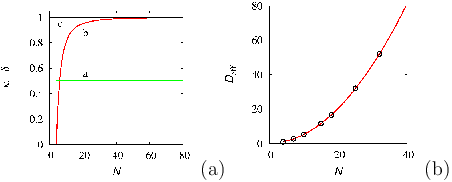
where for , and . Essentially, from state transitions occurs towards the two “nearest neighboring” states with equal probabilities. This model satisfy the velocity transition condition (60) for any . Moreover, the resulting structure tensor is isotropic for . Figure 8 panel (a) depicts the values of the two structure parameters and characterizing this model as a function of the number of stochastic velocity vectors considered. For this GPK process, for any , while approaches as increases, . Panel (b) of the same figure depicts the predicted value of the effective diffusivity given by eq. (70) taking . Symbols () corresponds to the estimate of from the scaling of the mean square displacements , along the and coordinates, , , obtained from stochastic simulations of eq. (21) with , using an ensemble of particles.
As another example consider the symmetric matrix
| (80) |
keeping the same stochastic velocity vectors (78). This model corresponds to the model analyzed by Kolesnik [93]. Since the structure is unchanged, for this model too. Also in this case, the velocity transition conditions (60) are satisfied, with , and the effective diffusivity, using eq. (70), is given by
| (81) |
in agreement with the analysis by Kolesnik [93]. If one slightly changes the transition probability matrix from eq. (80) to the form
| (82) |
one obtains , providing for any .

As can be observed, the fulfillment of the velocity transition condition is a fairly common property of many GPK processes.
Next, consider a system of nonuniform transition rates , , and a given transition matrix , and suppose that is a system of unit vectors satisfying the transition condition
| (83) |
with . Let
| (84) |
where is a parameter. By definition, the vectors defined by eq. (84) satisfy the transition condition eq. (72), so that the further requirement to be imposed on the transition rates is that also the zero-bias condition holds true, namely that
| (85) |
Eq. (85) represents a system of linear constraints on the admissible values of the transition rates . Once a system of admissible transition rates is determined via eq. (85), the resulting GPK process admits an effective diffusivity tensor the entries of which are given by
| (86) |
where, in the present case, the nominal diffusivity is . This implies that the parameter should be chosen such that . In this way, anisotropic diffusion processes can be generated in the Kac limit, corresponding to .
5.3 GPK in : construction of from platonic solid geometry
In , the construction of suitable vector systems , possessing enough symmetries to ensure the convergence towards isotropic diffusion in the Kac limit, can be grounded on the geometry of platonic solids. As well known, there are five platonic (regular) solids, possessing faces respectively: from corresponding to the tetrahedron, up to for the icosahedron.
Given a platonic solid possessing faces, the system of stochastic velocity vectors can be constructed by considering the normal unit vectors to the faces of the solid, multiplied by a characteristic velocity .
Consider uniform transition rates, i.e. , and the transition probability matrix expressed either by eq. (81) or by eq. (82).
For both the choices of the transition probability matrix, the transition conditions (60) amongst the vectors are satisfied, and the resulting diffusivity tensor is isotropic, namely , where .

In the case of (82), for all the five platonic solids in eq. (60), and . In the case of eq. (80) both and depend on , as depicted in figure 10. Observe that is a monotonic function of attaining the value for (tetrahedron), up to for (icosahedron).
The generalization to higher dimensional spaces can be obtained by applying the same procedure to higher dimensional polytopes.
6 Homogenization: the Kac limit as emerging property
So far we have analyzed the Kac limit as a limit behavior for and tending to infinity, keeping fixed the group . In point of fact, as purely stochastic dynamics is concerned, i.e., for , the convergence of GPK processes towards Brownian motion (Wiener processes) can be viewed as a long-term/large-distance property occurring for any value of and . The emerging Brownian-motion behavior characteristic of GPK processes is analyzed in this Section, using moment analysis, which is a classical technique in homogenization theory [100]. We show that in the long-term limit the statistical characterization of a GPK process approaches the solution of a parabolic model , where and are the constant effective velocity vector and diffusivity tensor, respectively, determining their values using the first elements of the moment hierarchy. Strictly speaking we do not prove the convergence, but rather we estimate and via first and second-order moment scaling. However, the complete proof of the convergence towards a parabolic model can be obtained using moment analysis and Pawula theorem [28], estimating the property of the fourth-order moments. This calculation is however extremely lengthy and is left to the tenacious reader.
6.1 Homogenization in the absence of a deterministic drift
Consider a GPK process in the absence of a deterministic drift, i.e., . In the analysis of the long-term properties assume also the following conditions: (i) the matrix is symmetric; (ii) the stochastic velocity vectors satisfy the zero-bias condition (28).
The concept of long-term property can be made quantitative: Consider the symmetric transfer matrix controlling the dynamics of state recombination. It admits as the dominant eigenvalue, which is non degenerate (single multiplicity) because the assumption of irreducibility. Let be the second eigenvalue with reversed sign. The characteristic time for relaxation of the state dynamics of the -state finite Poisson process generating the dynamics is therefore , so that long-term dynamics implies .
As stated above, consider a GPK process in the absence of a deterministic drift, and the system of lower-order partial moments
| (87) | |||||
for , . The dynamics of the zero-th order partial moments is given by
| (88) |
For , , approach a uniform distribution with respect to
| (89) |
which follows from the symmetry of . The first-order moments are solution of the equations
| (90) |
Since converge to constant values, the long-term limit of the first-order moments is at most linear with time,
| (91) |
where and , , are constant coefficients to be determined. Substituting eqs. (91) into eqs. (90) the following conditions amongst the expansion coefficients are obtained in the long-time limit
| (92) |
| (93) |
Summing over in eq. (93), and enforcing the zero-bias condition for the stochastic velocity vectors one gets
| (94) |
But the sum at the left-hand side of eq. (93) is exactly the definition of the -th entry of the effective velocity vector, so that eq. (94) implies
| (95) |
Moreover, by the symmetry of the matrix , it follows that eq. (92) is satisfied by a uniform vector in , , and due to eq. (94), it follows that . Therefore,
| (96) |
Next, consider the second-order partial moments that satisfy the system of evolution equations
| (97) |
Due to the long-term properties of , the second-order moments are, for , at most quadratic in time, to the leading order
| (98) |
In point of fact, since , it follows that the coefficients are identically vanishing. At present, we do not need to enforce this property. The substitution of this expression into the balance equation (97) provides the system of relations amongst the expansion coefficients
| (99) |
| (100) |
| (101) |
At this stage it is necessary to assume some conditions on the stochastic velocity vectors . As done in Section 5, let us assume the velocity transition condition (72) with .
Summing over in eq. (99) provides
| (102) |
The right-hand side in eq. (102) is identically vanishing, because of eq. (96). But the term at the left-hand side of eq. (102) is just the prefactor of the quadratic contribution associated with the overall second-order moment . Since the first-order moments are asymptotically constant, eq. (102) implies that the overall covariance matrix scales in the long-term regime linearly with time , i.e.,
| (103) |
and that the sum over the states of is twice the entry of the effective diffusivity tensor . To obtain an expression for this quantity, use eq. (101)
| (104) |
The term at the right-hand side can be estimated enforcing eqs. (93) and (96), derived from the dynamics of the first-order moments. Multiplying eq. (93) by , summing over the states , and enforcing the velocity transition condition (72) one gets
| (105) | |||||
which provides for the expression
| (106) |
and for an expression identical to eq. (76).
Some concluding observations on the long-term properties follows from the moment analysis addressed in this paragraph. In the case of purely stochastic GPK processes, the asymptotic approach towards a Brownian-like behavior is not solely a mathematical property that holds in the Kac limit, letting and diverge, keeping fixed . It is also a long-term asymptotics of the process. This makes GPK processes particularly appealing in the description of the physical systems in all the cases where the stochastic fluctuations occur at characteristic time-scales definitely shorter than the observation time-scales. It is also remarkable that all the conditions derived in Section 5 have been naturally and simply re-derived using homogenization techniques in the long-term limit.
6.2 A generalization
Within the framework of homogenization theory it is comfortable to address the case where no velocity transition conditions are assumed, and the stochastic velocity vectors fulfills solely the zero-bias condition (28). Even in this more general setting it is possible to derive a long-term Brownian behavior of GPK processes. Enforcing the fact that the first-order partial moments saturates asymptotically, i.e., , it follows that identically so that the effective diffusivity tensor can be defined and, by eqs. (101)-(102), is expressed by
| (107) |
From eqs. (93) and (96) it follows that, for a fixed value of the index , the coefficients satisfy a linear system of equations
| (108) |
where we have set and . Eqs. (108) represent decoupled systems of linear equations for , , the coefficient matrices of which are singular.
The matrix is, by assumption, symmetric, so that it possesses a system of real eigenvalues ordered such that , and of eigenfunctions ,
| (109) |
that can be always assumed to be mutually orthogonal and normalized to unit norm. The assumption of irreducibility implies that is non degenerate, so that , for . Specifically, the dominant eigenfunction is given by .
Let the usual Euclidean scalar product for -dimensional vectors , . The zero-bias condition on the velocity vectors implies that
| (110) |
for any . Therefore, the forcing terms in the linear systems (108) admit a vanishing projection onto the subspace spanned by the dominant (and vanishing) eigenvalue, and this ensures that eqs. (108) admit a solution, and indeed infinitely many. The solution of eq. (108) can be expressed by respect to the eigenfunctions of the coefficient matrix as
| (111) |
Substituting this expansion into eq. (108) after elementary algebra follows that for the expansion coefficients are univocally defined and given by
| (112) |
so that
| (113) |
depending on the arbitrary constants . The first term at the r.h.s of eq. (113) provides a vanishing contribution to the expression of the effective tensor diffusivity (107), due to the zero-bias conditions, so that the substitution of eq. (113) into eq. (107) provides the following expression for
| (114) |
representing the formal solution for the effective diffusivity tensor in the general case. From the above derivation it can be observed that, while the zero-bias condition represents a fundamental requisite in order to achieve an emergent Brownian behavior, the assumption of a given velocity transition condition is simply a very convenient property that provides an easy and compact expression for the Kac limit and for the emerging long-term properties, but that is not necessary for their occurrence, albeit in this general case the effective tensor diffusivity may not be isotropic.
6.3 Presence of a deterministic drift
In the previous paragraphs we have not considered the presence of a deterministic drift . This is because its presence may change completely the qualitative properties of GPK processes for small/moderate values of and .
The presence of a deterministic bias breaks down the symmetry between the Kac-limit in the parameter space and the long-term limit of GPK processes over all the range of parameters and . In point of fact this phenomenon can occur both for solenoidal and irrotational deterministic biasing fields .
Particularly critical is the case where is irrotational, i.e., it stems from a potential. In this case, it may happen that for small values of and the dynamics of a GPK process is not even ergodic, as it becomes trapped into many different invariant domains, each of which characterized by a unique stationary invariant probability density function. The phenomenon of ergodicity breaking is analyzed in [102] for one-dimensional Poisson-Kac dynamics, and thoroughly addressed in part II for higher dimensional systems.
6.4 A degenerate case: transitionally deterministic GPK processes
The assessment of the Kac limit for GPK processes goes well beyond the class of examples considered in paragraph 6.2. In this paragraph we consider another example that is interesting for highlighting other properties of GPK processes, represented by GPK models that are not transitionally symmetric, and that are associated with a rather peculiar transition mechanism: transition from any state occurs just towards a single one. For this reason, these models can be referred to as transitionally deterministic. More precisely, a GPK process is transitionally deterministic if there exists a one-to-one mapping such that
| (115) |
A transitionally deterministic process is irreducible, if the iterates of starting from any state spam the whole set of possible states .
A peculiar case of transitionally deterministic GPK processes is the one-dimensional Poisson-Kac process analyzed in Section 2, where the stochastic forcing is strictly dichotomic. This occurs because the number of distinct states equals . In this case, the process is also transitionally symmetric. The latter property however does not hold for .
Transitionally deterministic processes are interesting for the following reason: albeit the strictly deterministic transition mechanism, the long-term dynamics possesses a dissipative character, corresponding to the Kac limit. This is essentially due to the continuous time parametrization, which implies that, at any time , there is a finite probability of remaining at a given state , not switching to the state , and this provides an asymptotic dispersive behavior.
Below, we consider a subclass of these processes for which: (i) all the transition rates are equal , (ii) the velocity vectors satisfy the zero bias condition eq. (28), and finally, (iii) the process is velocity symmetric with the property that there exists an integer such that
| (116) |
where is the -th iteration of the map starting from state . Condition (iii) is not necessary to provide a Kac limit, but simplifies significantly the analysis.
The balance equations for the partial probability waves in transitionally deterministic GPK processes, characterized by uniform transition rates, read
| (117) |
where is the inverse mapping of . The diffusive flux is the solution of the equation
| (118) | |||||
where
| (119) |
Set
| (120) |
where . The balance equation for , , can be obtained multiplying eq. (117) by and summing over
| (121) | |||||
Summing over from up to
| (122) |
where we have set , . Enforcing property (iii), it follows that . Therefore, setting in eq. (122), and enforcing the infinitely fast partial-wave recombination, , one obtains the constitutive equation for the diffusive flux in the Kac limit
| (123) |
where, in the present case, the structure tensor is given by
| (124) |
Observe that the structure tensor defined by eq. (123) needs not to be symmetric. Eqs. (123)-(124) provide the expression for the Kac limit of this class of GPK processes.

Consider a practical example in . Let the stochastic velocity vectors be given by eq. (78) with , and the mapping be
| (125) |
For even and greater than 2, property (iii) is satisfied by . In this case, the direct calculation of the entries of the structure tensor provides
| (126) |
so that the resulting GPK process admits an isotropic Kac limit with
| (127) |
Figure 11 depicts the mean square displacement vs obtained from stochastic simulations of this GPK process in the absence of a deterministic bias, i.e., (an identical result can be obtained if would be considered) at . Panel (a) addresses the case at different values of , while panel (b) depicts the Kac limit for at increasing values of , keeping fixed . The following observations follow from the inspection of these data: (i) the estimate (127) is in perfect agreement with the numerical simulations, as for , and thus ; (ii) also for this class of processes, the Brownian-motion limit corresponds to an emerging long-term property, occurring for any value of and , although the characteristic time to reach this limit strongly depends on , and significantly increases with the number of states considered; (iii) at short-time scales, and for high values of , exhibits an oscillatory behavior, deriving from the circulant nature of the transition matrix which possesses a complex conjugate second eigenvalue.
7 Concluding remarks
GPK processes represent a very versatile generalization of the original Kac’s model of telegrapher’s noise extended to higher dimensional systems. They provide a broad class of stochastic processes possessing finite propagation velocity and, consequently, smooth (almost everywhere differentiable) trajectories. Their statistical description involves partial probability density functions, satisfying a hyperbolic system of equations with partial wave recombination, modulated by the transition probability matrix and by the transition rates . This “augmented” statistical description can be applied to ground, on stochastic microdynamic basis, the transport models of extended thermodynamic theory (see part III).
In this first part of the work we have analyzed the structural properties of GPK processes, i.e., how the structural features of the stochastic velocity vectors , of the transition probability matrix and of the transition rate vector impact on the Kac limit and on the the long-term properties of the dynamics.
In the absence of deterministic biasing fields, there is a strict correspondence between the Kac-limit behavior occurring for , keeping fixed the value of , and the long-term behavior for any finite values of and , providing the same value of , for time scales . Therefore, the Kac limit (and specifically the convergence towards classical parabolic transport schemes) is an emergent feature of GPK models.
Attention has been focused on the Kac limit which is a fundamental requisite connecting GPK processes to classical stochastic models driven by Wiener perturbations. A useful tool to derive the Kac limit behavior has been the transition condition (60) connecting the transition probability matrix to the structure of the velocity vectors .
All the physical implications of GPK dynamics and their extensions/generalizations are thoroughly addressed in part II and III of this work.
Appendix A Appendix
The cornerstone of the theory of hyperbolic and undulatory transport is represented by the model proposed by Kac [39] in one spatial dimension, and referred by the author as “telegrapher’s noise”. It is a Langevin equation where, instead of a stochastic perturbation expressed as the increment of a Wiener process, a Poisson-driven fluctuation dynamics is considered.
Let , , be a Poisson process, describing the number of events of a stationary, memoryless, ordinary stochastic process in the time interval . The process is described by the probability that an event occurs in the time interval , given by
| (128) |
where . It follows from eq. (128) the balance equations for the probabilities ,
| (129) |
where , out of which the Poissonian statistics, follows setting .
Let a deterministic velocity field , a characteristic velocity, and consider the stochastic differential equation
| (130) |
equipped with the initial condition , where is the above mentioned Poisson process. The stochastic perturbation in eq. (130) acts by switching from , to . Eq. (130) is referred to as the Poisson-Kac equation, and the associated process as the Poisson-Kac process.
Since the stochastic perturbation should not possess any bias for any , it is natural to assume the following initial conditions for the Poisson process
| (131) |
and zero otherwise, i.e., , . In such as way, for all , where indicates expectation values. From the initial condition (131), it follows that
| (132) |
where is a discrete Heaviside function for , for .
Therefore, , , and the correlation function for of the stochastic perturbation driving the Langevin equation (130) decays in time as
| (133) |
where . As flips between , depending on the parity of , this model of noise has been referred to as two-state dichotomous noise, and since its correlation function decays exponentially with time , it has been considered as one of the basic prototypes for colored noise.
Albeit these two properties are certainly important, the most relevant feature of the Poisson-Kac model is the finite-propagation velocity of the stochastic perturbation (provided that is sufficiently smooth, e.g. ), and this reflects into the fact that the trajectories of the stochastic process (the small case symbol indicates a realization of it) are almost everywhere differentiable functions of time [101].
If , eq. (130) becomes , while if , it reduces to . Therefore, the statistical description of can be grounded on the system of two partial probability density functions , defined as
| (134) |
and fulfilling the system of two first-order dissipative hyperbolic equations
| (135) |
The partial probability density functions are also referred to as the two partial probability waves of the Poisson-Kac process. The finite propagation is ensured by the bounded values of , while dissipation is accounted for by the recombination dynamics amongst the partial waves. Indicating with the overall probability density function for at time , and with the probability flux associated with the Poissonian stochastic perturbation (i.e., the “diffusive flux” in the Poisson-Kac model),
| (136) |
it follows from eq. (135) that
| (137) |
If , the second equation (137) corresponds to a Cattaneo constitutive equation. This is the reason why the Cattaneo equation, and the Poisson-Kac process in the absence of a deterministic bias, i.e., , have been considered essentially as two descriptions (Eulerian vs Lagrangian) of the same physics. This is not always true as boundary conditions enters in the picture, and the probabilistic interpretation of the Cattaneo equation, even in one-dimensional spatial problems, poses strict and quantitative constraints on the nature of the admissible boundary conditions [91].
Nevertheless, even in one spatial dimension, the analogy breaks down if , and does not occur for spatial dimensions higher than . More precisely, the Cattaneo constitutive equation for ,
| (138) |
where are constants, , does not correspond to any stochastic process. Correspondingly, the substitution of this constitutive equation into the balance equation , leads to an evolution equation for , that starting from a non-negative initial probability density , may lead at some time to negative values of [69].
The other important property of the Poisson-Kac model is its asymptotic limit, whenever and are let to diverge , keeping fixed the ratio
| (139) |
Under these conditions, the second equation (137) reduces to a Fickian form (we use the diction “Fickian” to indicate any constitutive equation where the diffusive flux is proportional to the gradient of the density),
| (140) |
and the probability balance equation (first equation (137)) converges to the classical parabolic advection-diffusion equation
| (141) |
We refer to this limit as the Kac limit, which implies that:
- •
a classical Langevin equation driven by a Wiener process can be always regarded as the Kac limit of some Poisson-Kac dynamics;
- •
References
- [1] Kleinert H 1988 Gauge fields in condensed matter Vol. 1 (Singapore: World Scientific)
- [2] Zinn-Justin J 1988 Quantum field theory and critical phenomena (Oxford: Oxford Science Publ.)
- [3] Nelson E 1985 Quantum fluctuations (Princeton: Princeton University Press)
- [4] Feynman R and Hibbs A R 2010 Quantum mechanics and path integrals (New York: Dover Publ.)
- [5] Kleinert H 2009 Path integrals in quantum mechanics, statistics, polymer physics and financial markets (Singapore: World Scientific)
- [6] Chandrasekhar S 1943 Rev. Mod. Phys. 15 1
- [7] Öttinger H C 1996 Stochastic Processes in Polymeric Fluids (Berlin: Springer Verlag)
- [8] Doi M and Edwards S F 1988 The theory of polymer dynamics (Oxford: Oxford Univ. Press)
- [9] de Groot S R and Mazur P 1984 Non-equilibrium thermodynamics (New York: Dover Publ.)
- [10] Kondepuni D and Prigogine I 2014 Modern Thermodynamics (Chichister, J. Wiley & Sons)
- [11] Falconer K J 1986 The geometry of fractal sets (Cambridge: Cambridge Univ. Press)
- [12] Zwanzig R 1961 Phys. Rev 124 983
- [13] Cattaneo C 1948 Atti Semin. Mat. Fis. Univ. Modena 3 3
- [14] Cattaneo C 1958 Compt. Rend. 247 431
- [15] Vernotte P 1958 Comp. Rend. 246 3154
- [16] Simons S 1973 J. Phys. A 6 1543
- [17] Lebon G, Ruggieri M and Valenti A 2008 J. Phys. Condens. Matter 20 025223
- [18] Christov C I and Jordan P M 2005 Phys. Rev. Lett. 94 154301
- [19] Christov C I 2009 Mech. Res. Comm. 36 481
- [20] Cimmelli V A, Sellitto A and Jou D 2010 Phys. Rev. B 81 054301
- [21] Jou D and Cimmelli V A 2016 Commun. appl. Ind. Math. 7 196
- [22] Joseph D D and Preziosi L 1989 Rev. Mod. Phys. 61 41
- [23] Ruggeri T, Muracchini A and Seccia L 1990 Phys. Rev. Lett. 64 2640
- [24] Tung M M, Trujillo M, Molina J L, Rivera M J and Berjano E J 2009 Math. Comp. Modell. 50 665
- [25] Jou D, Sellitto A and Cimmelli V A 2014 Int. J. Heat Mass Transf. 71 459
- [26] Olivares-Robles M A and Garcia-Colin L S 1994 Phys. Rev. E 50 2451
- [27] Olivares-Robles M A and Garcia-Colin L S 1996 J. Non-Equilib. Thermodyn. 21 361
- [28] Pawula R F 1967 Phys. Rev. 162 186
- [29] Zhang Z M, Bright T J and Peterson G P 2011 Nano. Micro. Thermophys. Eng. 15 220.
- [30] Metzler R and Compte A 1999 Physica A 268 454
- [31] Grad H 1949 Comm. Pure Appl. Math. 2 331
- [32] Müller I 1967 Z. Phys. 198 329
- [33] Müller I and Ruggeri T 2013 Rational extended thermodynamics (New York: Springer Science & Business Media)
- [34] Müller I 1999 Living Rev. Relativity 2 1
- [35] Garcia-Colin L S, Lopez de Haro M, Rodriguez R F, Casas-Vazquez J and Jou D 1984 J. Stat. Phys. 37 465
- [36] Jou D, Casas-Vazquez J and Lebon G 1988 Rep. Prog. Phys. 51 1105
- [37] Jou D, Casas-Vazquez J and Lebon G 1999 Rep. Prog. Phys. 62 1035
- [38] Jou D, Casas-Vazquez J and Lebon G 1996 Extended irreversible thermodynamics (Berlin: Springer Verlag)
- [39] Kac M 1974 Rocky Mount. J. Math. 4 497
- [40] Goldstein S 1951 Quart. J. Mech. Appl. Math. 4 129
- [41] Sancho J 1984 J. Math. Phys. 25 354
- [42] Pawula R F 1987 Phys. Rev. A 35 3102
- [43] Masoliver J, Porrá J M and Weiss G H 1993 Phys. Rev. E 48 939
- [44] Masoliver J and Weiss G H 1994 Phys. Rev. E 49 3852
- [45] Dean Astumian R and Bier M 1994 Phys. Rev. Lett. 72 1766
- [46] Porrá J M and Lindenberg K 1995 Phys. Rev. E 52 409
- [47] Fulinski A 1995 Phys. Rev. E 52 4523
- [48] Masoliver J and Weiss G H 1996 Eur. J. Phys. 190
- [49] Reimann P and Elston T C 1996 Phys. Rev. Lett. 77 5328
- [50] Boguna M, Porrá J M and Masoliver J 1999 Phys. Rev. E 59 6517
- [51] Laio F, Ridolfi L and D’Odorico P 2008 Phys. Rev. E 78 031137
- [52] Arnold L, Horsthemke W and Levefer R 1978 Z. Phys. B 29 367
- [53] Kus M, Wajnryb E and Wodkiewicz K 1991 Phys. Rev. A 43 4167
- [54] Hänggi P and Jung P 1995 Adv. Chem. Phys. 89 239
- [55] Kim S, Park S H and Ryu C S 1998 Phys. Rev. E 58 7994
- [56] Weiss G H 2002 Physica A 311 381
- [57] Bena I 2006 Int. J. Mod. Phys. B 20 2825
- [58] Horsthemke W and Lefever R 2006 Noise-Induced Transitions (Berlin: Springer Verlag)
- [59] Kitahara K, Horsthemke W and Lefever R 1979 Phys. Lett. A 70 377
- [60] Kitahara K, Horsthemke W, Lefever R and Inaba Y 1980 Prog. Theor. Phys. 64 1233
- [61] Horsthemke W, Doering C R, Lefever R, and Chi A S, 1985 Phys. Rev. A 31 1123
- [62] Müller R, and Behn U 1990 Z. Phys. B 78 229
- [63] Gaveau B, Jacobson T, Kac M and Schulman L S 1984 Phys. Rev. Lett. 53 419
- [64] Kudo T and Ohba I 2002 Praman 59 413
- [65] Balakrishnan V and Lakshmibala S 2005 New J. Phys. 7 11
- [66] Srinivasan S K and Sudarshan E C G 1996 J. Phys. A 29 5181
- [67] Beccaria M, Presilla C, De Angelis G F and Jona-Lasinio G 1999 Europhys. Lett. 48 243
- [68] Beccaria M, Presilla C, De Angelis G F and Jona-Lasinio G 2001 Int. J. Mod. Phys. B 15 1740
- [69] Körner C and Bergmann H W 1998 Appl. Phys. A 67 397
- [70] Bright T J and Zhang Z M 2009 J. Thermophys. Heat Transf. 23 601
- [71] Vavruch I 2002 Chemické listy 96 271
- [72] Dunkel J and Hänggi P 2009 Phys. Rep. 471 1
- [73] Zhukovsky K 2016 Int. J. Heat Mass Transf. 98 523
- [74] Kolesnik A D 2008 J. Stat. Phys. 131 1039
- [75] Kolesnik A D and Pinsky M A 2011 J. Stat. Phys. 142 828
- [76] Masoliver J, Porrà J M and Weiss G H 1992 Physica A 192 593
- [77] Masoliver J, Porrà J M and Weiss G H 1993 Physica A 193 469
- [78] Boguna M, Porrà J P and Masoliver J 1998 Phys. Rev. E 58 6992
- [79] Godoy S and Garcia-Colin L S 1997 Phys. Rev. E 55 2127
- [80] Giona M, Brasiello A and Crescitelli S 2016 Stochastic foundations of undulatory transport phenomena: Generalized Poisson-Kac processes - Part II Irreversibility, Norms and Entropies, submitted to J. Phys. A
- [81] Giona M, Brasiello A and Crescitelli S 2016 Stochastic foundations of undulatory transport phenomena: Generalized Poisson-Kac processes - Part III Extensions and applications to kinetic theory and transport, submitted to J. Phys. A
- [82] Rosenau P 1993 Phys. Rev. E 48 R655
- [83] Giona M, Brasiello A and Crescitelli S 2016 J. Non-Equil. Thermodyn. 41 107
- [84] Kac M 1956 Foundations of kinetic theory, in Proc. 3rd Berkeley Symp. Math. Stat. Prob., J. Neyman (Ed.), Univ of California, vol. 3, 171
- [85] Mischler S and Mouhot C 2013 Invent. Math. 193 1
- [86] Michler S 2013 Kac’s chaos and Kac’s program, arXiv preprint arXiv:1311.7544
- [87] Doolen G et al. (Eds.) 1990 Lattice Gas Methods for Partial Differential Equations (Menlo Park: Addison-Wesley)
- [88] Cabennes H, Gatisgnol R and Luo L S 2003 The discrete Boltzmann equation (Berkeley: University of California)
- [89] Palczewski A and Schneider J 1998 J. Stat. Phys. 1998 307
- [90] Vinerean M C, Windfäll A and Bobylev A V 2010 Nuovo Cimento 33 257
- [91] Brasiello A, Crescitelli S and Giona M 2016 Physica A 449 176
- [92] Giona M 2016 Covariance and spinorial statistical description of simple relativistic stochastic kinematics, in preparation
- [93] Kolesnik A D and Turbin A F 1998 Stoch. Proc. Appl. 75 67
- [94] Guyer R A and Krumhansl J A 1966 Phys. Rev. 148 766
- [95] Guyer R A and Krumhansl J A 1966 Phys. Rev. 148 778
- [96] Cimmelli V A and Frischmuth K 2007 Physica B 400 257
- [97] Plyukhin A V 2010 Phys. Rev. E 81 021113
- [98] Seneta E 2006 Non-negative matrices and Markov Chains (New York: Springer Science & Business Media)
- [99] Giona M, Brasiello A and Crescitelli S 2016 Markovian nature, completeness, regularity and correlation properties of Generalized Poisson-Kac processes, submitted to J. Sta. Mech.
- [100] Brenner H and Edwards D A 1993 Macrotransport Processes (Boston: Butterworth-Heinemann)
- [101] Giona M, Brasiello A and Crescitelli S 2016 Physica A 450 148
- [102] Giona M, Brasiello A and Crescitelli S 2015 Europhys. Lett. 112 30001
- [103] Wong E and Zakai M 1965 Int. J. Eng. Sci. 3 213
- [104] Wong E and Zakai M 1965 Ann. Math. Stat. 36 1560