Gravitational lens system SDSS J1339+1310: microlensing factory and time delay
Abstract
We spectroscopically re-observed the gravitational lens system SDSS J1339+1310 using OSIRIS on the GTC. We also monitored the -band variability of the two quasar images (A and B) with the LT over 143 epochs in the period 20092016. These new data in both the wavelength and time domains have confirmed that the system is an unusual microlensing factory. The C iv emission line is remarkably microlensed, since the microlensing magnification of B relative to that for A, , reaches a value of 1.4 ( 0.4 mag) for its core. Moreover, the B image shows a red wing enhancement of C iv flux (relative to A), and = 2 (0.75 mag) for the C iv broad-line emission. Regarding the nuclear continuum, we find a chromatic behaviour of , which roughly varies from 5 (1.75 mag) at 7000 Å to 6 (1.95 mag) at 4000 Å. We also detect significant microlensing variability in the band, and this includes a number of microlensing events on timescales of 50100 d. Fortunately, the presence of an intrinsic 0.7 mag dip in the light curves of A and B, permitted us to measure the time delay between both quasar images. This delay is = 47 d (1 confidence interval; A is leading), in good agreement with predictions of lens models.
Key Words.
gravitational lensing: strong – gravitational lensing: micro – cosmological parameters – quasars: individual: SDSS J1339+13101 Introduction
If there is a massive galaxy between a distant quasar and the Earth, the quasar is seen as a multiple system consisting of several images (Schneider et al., 1992, e.g.). This gravitationally lensed quasar may also suffer microlensing effects by stellar mass objects in the lensing galaxy. Quasar microlensing was firstly detected in 1989 (Irwin et al., 1989; Vanderriest et al., 1989), and has become a powerful astrophysical tool in the current century (Schneider et al., 2006, e.g.). Microlensing particularly affects compact sources such as the X-ray emitting regions, the accretion disk or the innermost line emitting clouds, so microlensed quasars are being intensively used to probe the quasar structure from spectral studies (Chartas et al., 2004; Richards et al., 2004; Pooley et al., 2007; Sluse et al., 2007; Bate et al., 2008; Floyd et al., 2009; Blackburne et al., 2011; Mediavilla et al., 2011; Mosquera et al., 2011; Muñoz et al., 2011; Jiménez-Vicente et al., 2012; Motta et al., 2012; Sluse et al., 2012; Guerras et al., 2013; Braibant et al., 2014; Jiménez-Vicente et al., 2014; Rojas et al., 2014; Sluse et al., 2015, e.g.) and analyses of extrinsic variabilities (Chartas et al., 2002; Shalyapin et al., 2002; Goicoechea et al., 2003; Kochanek, 2004; Gil-Merino et al., 2006; Morgan et al., 2006; Paraficz et al., 2006; Eigenbrod et al., 2008; Morgan et al., 2008a; Morgan et al., 2008b; Poindexter et al., 2008; Chartas et al., 2009; Dai et al., 2010; Morgan et al., 2010; Poindexter & Kochanek, 2010; Chen et al., 2011; Sluse et al., 2011; Chartas et al., 2012; Chen et al., 2012; Morgan et al., 2012; Hainline et al., 2013; Mosquera et al., 2013; Blackburne et al., 2014; Blackburne et al., 2015; MacLeod et al., 2015; Mediavilla et al., 2015a; Mediavilla et al., 2015b, e.g.).
Unfortunately, many lensed quasars have only experienced weak microlensing effects in their spectra and light curves. Thus, it is important to identify the systems showing substantial spectral distortions due to microlensing, sharp microlensing variations or both phenomena. These microlensing factories are excellent tools for detailed interpretations, as well as the best targets for subsequent follow-up through suitable facilities (Mosquera & Kochanek, 2011, e.g.). For example, some systems exhibited strong chromatic microlensing in the optical continuum, with a maximum signal of 0.8 mag at 5439 Å (Rojas et al., 2014, HE 00471756 and SDSS J1155+6346;). A microlensing-induced distortion of the shape of several high-ionization emission lines was also unambiguously detected in SDSS J1004+4112 (Richards et al., 2004; Motta et al., 2012, e.g.). Additionally, the Einstein Cross (QSO 2237+0305) displayed prominent microlensing (extrinsic) events in its -band light curves over the final years of the past century (Woźniak et al., 2000; Udalski et al., 2006), and these 0.7 mag variations on hundreds of days strongly stimulated interpretation tasks and further observations (see above).
Lensed quasars are not only powerful laboratories of the quasar structure, but are also often used as a cosmological probe (Refsdal, 1964; Schneider et al., 2006, e.g.). For that purpose, the time delay between pairs of lensed images must be measured to high accuracy, requiring us to disentangle extrinsic and intrinsic variability. Intrinsic variations in a lensed quasar appear in two given images at different observing times, and a measurement of the time delay between these lensed images can be used to estimate the current expansion rate of the Universe (the so-called Hubble constant) and other cosmological parameters (Oguri, 2007; Suyu et al., 2010; Suyu et al., 2013; Sereno & Paraficz, 2014; Rathna Kumar et al., 2015, e.g.). The time delay is also sensitive to the distribution of the lensing mass (Refsdal, 1964; Schneider et al., 2006; Goicoechea & Shalyapin, 2010, e.g.), so time delay measurements are turning in critical data for cosmology and extragalactic astrophysics. However, lensed quasars with appreciable extrinsic variations in their optical light curves may be a challenge for time delay determinations, since, in general, the extrinsic variability should be modelled by microlensing simulations or appropriate functions (e.g. Tewes et al., 2013a, and references therein).
Various techniques have been developed to deblend the intrinsic signal from the microlensing variability. However, as seems intuitive, if the intrinsic and extrinsic variations have similar timescales and amplitudes, it is not possible to fairly distinguish between both signals and accurately determine the time delay of a lens system (Morgan et al., 2008a; Morgan et al., 2012, e.g. Q J01584325;). Despite the presence of clear extrinsic variability in HE 11041805, the time delay between its two images was measured to 4% precision (Ofek & Maoz, 2003, 1 confidence interval;). Ofek & Maoz (2003) modelled a long-term microlensing gradient and analised the influence of short-timescale microlensing events (having a mean amplitude of 0.07 mag and a duration of approximately 1 month) in the delay estimation. Using additional data, and Legendre polynomials for describing the intrinsic and extrinsic variabilities, the relative uncertainty in the time delay measurement was decreased to 2% (Poindexter et al., 2007). For this system (HE 11041805), Morgan et al. (2008a) also re-estimate the delay by modelling the extrinsic fluctuations through microlensing simulations. They obtained an 1 confidence interval in very good agreement with the Ofek & Maoz’s measurement. More recently, Tewes et al. (2013b) and Rathna Kumar et al. (2013) modelled the long-timescale extrinsic variations of two lens systems (RX J11311231 and SDSS J1001+5027) by free-knot splines (among other techniques), incorporating short-timescale correlated noise in their analyses. They measured the longest delays with 2% precision. Hainline et al. (2013) also modelled the microlensing fluctuations in SBS 0909+532 by intensive simulations. The light curves of this double quasar included an intrinsic deep dip and significant extrinsic variability on different timescales, allowing the authors to estimate the 50-d delay with 6% precision.
As a part of the road map to deeply analyse the system SDSS J1339+1310, this paper is mainly dedicated to characterising the microlensing signal in the wavelength and time domains, as well as to measure the time delay. The lens system SDSS J1339+1310 consists of two quasar images (A and B) at the same redshift = 2.231 and separated by 170, as well as a lensing galaxy (G) at = 0.609 and located 063 from the B image (Inada et al., 2009; Shalyapin & Goicoechea, 2014). While A and B are optically bright ( 1819 mag), the galaxy G has an -band magnitude of about 20.5. Spectra of the lens system were obtained in 2013 using the OSIRIS R500R grism on the 10.4 m Gran Telescopio Canarias (GTC). These GTC-OSIRIS spectra allowed us to measure the redshift of G and obtain constraints on the macrolens and extinction parameters (Shalyapin & Goicoechea, 2014, henceforth Paper I). We also found evidence for strong chromatic microlensing in its optical continuum (reaching a maximum signal of 1.51.7 mag at 5000 Å), and were able to predict a time delay between A and B of 4050 d (A is leading). The presence of sharp extrinsic events in preliminary light curves with the 2.0 m Liverpool Telescope (LT) precluded direct measurement of the delay.
In Sect. 2, we present new high-quality GTC (optical) spectra of A, B and G in 2014. In Sect. 3, we discuss widely the several spectral distortions caused by microlensing. In Sect. 4, we also present -band LT light curves of A and B in 2009, 20122015 and early 2016. In Sect. 5, these curves are used to estimate the time delay and the -band microlensing variability. Our conclusions are summarised in Sect. 6. We also include two appendices to address some specific issues.
2 Spatially resolved spectroscopy
To improve the spectroscopic information of SDSS J1339+1310, 3570 (31190) s GTC-OSIRIS exposures of the lens system were taken on 27 March 2014 (R500R grism) and 20 May 2014 (R500B grism). The slit was oriented along the line joining both quasar images A and B, and the slit width was 123 ( 5 pixel). We used IRAF11 1 IRAF is distributed by the National Optical Astronomy Observatory, which is operated by the Association of Universities for Research in Astronomy (AURA) under cooperative agreement with the National Science Foundation. This software is available at http://iraf.noao.edu/ packages to perform usual data reductions, and the raw and reduced spectral frames in FITS format are publicly available at the GTC archive22 2 http://gtc.sdc.cab.inta-csic.es/gtc/index.jsp. The new 1 h exposures are longer than the previous one with the R500R grism (85). The new data also cover a broader wavelength range of 36009260 Å (Cabrera-Lavers, 2014, the fringing and second-order contamination become relevant from about 9300 Å redward; see sections 6.3 and 6.7 of). Additionally, the seeing conditions in 2014 were better than those in 2013, since we estimated seeing values of 08, 09 and 11 for the three dithered sub-exposures with the red grism (7000 Å), and 09, 09 and 10 for the sub-exposures with the blue grism (4745 Å). The spectral resolution of the two grisms was evaluated from the widths of the bright sky line at 5557 Å, resulting in resolving powers of 290 ( = 19.2 Å; red grism R500R) and 367 ( = 15.2 Å; blue grism R500B).
Before presenting the extraction of spectra for the three sources (A, B and G), we want to briefly discuss the differential atmospheric refraction (DAR) in our observations. This atmospheric phenomenon may cause a substantial chromatic offset of sources across the slit (transverse direction), leading to undesirable spectral artefacts (Filippenko, 1982). The amplitude of the wavelength-dependent transverse offset is related to the airmass and the slit position angle with respect to the zenith. Thus, the higher is the airmass and the farther the zenith is oriented the slit, the larger is the amplitude of the transverse offset. For the three GTC-OSIRIS sub-exposures with the red grism, the values of the airmass and the slit position angle were (1.223, 1.294, 1.383) and (18, 40, 56), respectively. For the blue grism sub-exposures, the airmass was lower (1.056, 1.076, 1.105), while the position angle was larger (249, 152, 82). From these data, considering on-axis quasar images at 6200 Å (acquisition frames were taken in the SDSS passband), the maximum transverse shifts of sources are 005 (red grism) and 02 (blue grism), and significant spectral distortions induced by DAR are not expected. The maximum spectral deviation by slit loss occurs on the blue edge of the blue grism, where a transverse shift of 02 induces a deviation of a few percent. This artefact is removed when calculating the spectral ratio in the bluest region. The spectral ratio is essentially free from DAR artefacts, because the two involved spectra are equally affected (same grism) or weakly affected (region of overlap between both grisms at 48507200 Å) by DAR.
The extraction of individual spectra of A, B and G is not a so direct task, and we followed the procedure that was presented and exhaustively discussed in 85. Our technique is a variant of the approach by Sluse et al. (2007) to produce spectra of sources in a crowded region. We initially modelled the lens system as a 2D light distribution including two point-like sources (A and B) and a de Vaucouleurs profile (G). This ideal model relied on the astro-photometric constraints in the last column of Table 1 of 85. The initial light distribution was then convolved with a 2D Moffat function, masked with the slit transmission and integrated across the slit. The final (realistic) 1D model at each wavelength depends on the position of A, the shape of the Moffat profile, and the fluxes of A, B and G. After some iterations (fits to the 1D data for each wavelength bin), we extracted the instrumental fluxes of the three sources throughout the entire spectral range of each individual frame (sub-exposure). The basic response curves (red and blue grisms) to calibrate the flux scales were derived from spectroscopic observations of the standard stars Hilt600 and GD153. Each star was modelled as a 2D Moffat distribution at each wavelength. These distributions were masked with the slit transmission, integrated across the slit and compared to the 1D observed profiles. The basic responses were then corrected by airmass differences to get a response curve for each individual frame of the lens system. In a last step, the three instrumental spectra of each source for each grism were calibrated in flux and combined into a single spectral energy distribution.
The final spectra of A, B and G are available in tabular format at the CDS33 3 See also http://grupos.unican.es/glendama/q1339.htm: Table 1 includes wavelengths in Å (Col. 1), and fluxes of A, B and G in 10-17 erg cm-2 s-1 Å-1 (Cols. 2, 3 and 4) from the red grism data, while Table 2 is structured in the same manner as Table 1, but incorporating the spectra associated with the blue grism. The results from the observations with both grisms are also plotted in Fig. 1. In this figure, we show the spectra of A (red), B (blue) and G (green). Bright colours trace the R500R spectra at the first observing epoch, whereas light colours represent the R500B spectra at the second epoch, 50 d later. As expected, the new quasar spectra are much less noisy than those in 85, and incorporate many emission lines (vertical dotted lines). Here, in Sec. 3, we focus on the five resolved prominent features: Ly, Si iv/O iv], C iv, C iii] and Mg ii. Although a detailed study of the quasar absorption lines is out of the scope of this paper, several absorption features are also evident in the spectra of A and B. In Appendix A, we assess the quality of the spectral extraction, as well as the short-term evolution of the quasar spectral energy distribution.


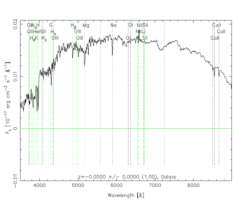
Regarding the lensing galaxy, we analysed the new spectra of G in Fig. 1 to better understand its nature. The RVSAO/XCSAO IRAF package (Kurtz & Mink, 1998) was used to perform the cross-correlation between these spectra and two different early-type galaxy templates. First, the improved spectrum from the red grism and the elliptical galaxy template in the Kinney-Calzetti Spectral Atlas of Galaxies (Kinney et al., 1996) led to a signal-to-noise ratio in the cross-correlation peak (Tonry & Davis, 1979, ;) of about 5, while reached a value of 8 using the spectrum from the blue grism. Second, taking the early-type galaxy template in the SDSS database44 4 http://classic.sdss.org/dr7/algorithms/spectemplates/spDR2-023.gif, we obtained values in the interval . The four measurements of the lens redshift (one for each combination spectrum-template) ranged between 0.607 and 0.608. In Fig. 2, we compare the two galaxy spectra with the red-shifted SDSS template (adopting = 0.607; see below). These GTC-OSIRIS spectra clearly show several absorption features (e.g. the Ca ii doublet and the G-band are unambiguously detected with both grisms), which allowed us to estimate values close to 0.606. Thus, the data of G in 2014 lead to = 0.607 0.001 (1 interval). Although the new typical value of the lens redshift differs only in a 0.3% from the previous one in 85, we adopt the for the improved spectra. We did not try to fit stellar population synthesis models to the spectra, but the lack of [O ii] emission at 3727 Å (it would be observed at 6000 Å) is likely indicating a lack of star formation in the lensing galaxy (Kennicutt, 1998, e.g.).
3 Microlensing in the broad line and nuclear continuum emitting regions
GTC-OSIRIS-R500R spectroscopy of the doubly imaged quasar SDSS J1339+1310 in 2013, revealed the presence of strong chromatic microlensing of its continuum, which is primarily generated in a nuclear region. In 85, we used the flux ratio for the cores of three emission lines (C iv, C iii] and Mg ii) to estimate the macrolens magnification and dust extinction ratios, and , and thus find the microlensing magnification ratio of light basically coming from the nuclear continuum emitting region (NCER). Our main hypothesis in this first paper was that the cores of emission lines are dominated by photons arising from the narrow line emitting region (NLER) and the outer parts of the broad line emitting region (BLER). Therefore, the line cores would be produced in extended regions that are unaffected by microlensing (e.g. Motta et al., 2012, and references therein).
The GTC-OSIRIS low-noise spectra of the lensed quasar in 2014 cover the whole range of optical wavelengths and contain five prominent emission features, that is the three previous lines and two additional features at bluer wavelengths (Ly and Si iv/O iv]; see Fig. 1). These new data offer a much richer information than those in 85, and are useful to check the hypothesis about microlensing-free fluxes of line cores (see Sec. 3.1 and Sec. 3.2), as well as to improve our knowledge on the extinction and magnification in SDSS J1339+1310 (see Sec. 3.2 and Sec. 3.3). We considered a number of details to analyse the optical spectra of A and B, including an accurate estimation of the total and nuclear power-law continua. The spectral energy distributions of the A image at 48507200 Å for the two spectroscopy epochs in 2014 are remarkably similar (see Fig. 1 and Appendix A), so we mainly used the blue grism data to estimate delay-corrected flux ratios over a very broad wavelength range (36007200 Å; it was implicitly assumed that the observed constancy of the spectrum of A in the and bands can be extended to the band). These delay-corrected ratios were complemented with two measurements from the red grism data: flux ratios of the C iii] and Mg ii line cores (a justification for the use of the two additional single-epoch ratios is provided at the end of Appendix A).
3.1 Microlensing-free fluxes of line cores?
We initially assumed that the line cores are unaffected by microlensing and only macrolens-extinction effects are playing a role (e.g. Motta et al., 2012, and references therein). In this scenario, due to differential dust extinction in the lensing galaxy, the line-core flux ratios and the associated magnitude differences are expected to have a certain chromatic behaviour. Using a standard formalism for the differential extinction of lensed images (Falco et al., 1999; Wucknitz et al., 2003; Elíasdóttir et al., 2006, e.g.), we presented two chromaticity laws in equations 23 of 85, which can be compared with the observed magnitude differences in Table 2. Although we were able to perfectly fit the Galactic law to the new data for the cores of the Mg ii, C iii] and C iv emissions ( 0; see the dotted red line in Fig. 3), a large value of was obtained by adding the magnitude difference for Si iv/O iv] ( 10 with 1 degree of freedom; see the dashed red line in Fig. 3). The fitting result was even worse when we used the five available differences ( 80 with 2 degrees of freedom; see the solid red line in Fig. 3).

Apart from the Galactic extinction (Cardelli et al., 1989), we also considered the simple linear law: , , as a second variant. This is a reasonable approach for dust extinction at 24 (Prévot et al., 1984, e.g.), that is in the spectral region of interest (see Fig. 3). The standard linear law did not fit significantly better than the Galactic law, since the five magnitude differences in Table 2 produced a still unacceptable chi-square value ( 80 with 3 degrees of freedom; see the solid green line in Fig. 3). Therefore, our analysis indicated the existence of a conflict between a macrolens-extinction scenario and the full dataset of values, and thus revealed that microlensing is affecting to some extent the emission line cores. Although we assumed that the line central features are dominated by photons arising from the NLER and the outer parts of the BLER, some of them contain an appreciable number of photons coming from clouds at inner zones of the BLER and moving almost perpendicularly to the line of sight (small projected motions).


The BLER is likely stratified, so different atoms or ions are located at different distances from the NCER. For example, there is evidence for a correlation between degree of ionization and distance, with the high-ionization species much closer to the NCER than those of low-ionization (Krolik et al., 1991; Gaskell et al., 2007, e.g.). In this standard stratification of the BLER (SSB), the C iv, Si iv/O iv] and Ly cores could suffer slight microlensing effects, while the Mg ii and C iii] cores would probably be free of microlensing (see Table 2). Hence, the low-ionization, outer lines of Mg ii and C iii] were used to obtain a macrolens-extinction solution (standard linear law), and remove macrolens and extinction effects in the cores of the C iv, Si iv/O iv] and Ly emissions. The best-fit solution was = 0.16 and = 1.44, and the microlensing magnification ratios of the C iv, Si iv/O iv] and Ly line cores are shown in the bottom panel of Fig. 4 (filled green circles). As expected, all the values are close to one.
In addition to a SSB, we also considered a non-standard stratification of the BLER (NSB): the typical distance from the central engine to a specie depends on the total energy that is required to produce each excited or ionised atom of such specie (the higher the energy of excitation or ionization, the distance is smaller). This naive scenario relies on the idea that the available amount of energy for excitation or ionization decreases with distance, leading to outer lines of Mg ii and Ly (see Table 2). We used these two lines to infer a new macrolens-extinction solution, = 0.19 and = 1.22, which allowed us to discuss the microlensing magnification ratios of the C iii], C iv and Si iv/O iv] line cores. It is noteworthy that we assumed = 1 (absence of microlensing) for the Mg ii and Ly lines (excitation energy of hydrogen and ionization energy of magnesium of 10 eV; see the open red circles in the bottom panel of Fig. 4), and then obtained a microlensing signal 1 for the other lines (see the filled red circles in the bottom panel of Fig. 4), with a clear correlation between the values and the ionization energies (i.e. 0.08/35 (C iii]), 0.34/80 (C iv) and 0.25/60 (Si iv/O iv]) eV-1). This correlation is fully consistent with the NSB scenario.
3.2 Microlensing in the BLER
To estimate a reliable macrolens-extinction solution, the ideal procedure is to use pure narrow lines arising from the NLER (Moustakas & Metcalf, 2003, e.g.), instead of line cores presumably unaffected by microlensing (e.g. the SSB and NSB scenarios give two solutions slightly different from each other; see above). Unfortunately, these pure narrow lines are not available yet, so we performed the decomposition of the carbon lines to get a robust solution. The C iii] and C iv emission lines are located within the central region of the full range of wavelengths, and their signal strengths are enough as to do decompositions into broad and narrow components. With a little more detail, our decomposition is based on the blue grism spectra of the lensed quasar SDSS J1339+1310. After de-redshifting the spectra to their rest frame, apart from continuum subtractions, each line profile was modelled as a sum of Gaussian contributions (see below). A multi-component decomposition of line profiles has been used in many previous works with different aims (Wills et al., 1985; Kuraszkiewicz et al., 2002; Dietrich et al., 2003; Sluse et al., 2007; Marziani et al., 2010, e.g.), and recently, Sluse et al. (2011) identified and studied different components of the C iii] and C iv lines in spectra of the gravitationally lensed quasar Q2237+0305.
To reproduce the C iii]1909 profile in each quasar image, after some probes, we used two C iii] components (broad and narrow), plus two blue-wing excesses due to Si iii]1892 and Al iii 1857 emissions (Brotherton et al., 1994, e.g.). Each of these four Gaussian components is characterised by three parameters: central wavelength , width (standard deviation) and amplitude. The C iii], Si iii] and Al iii emissions were fixed at = 1908.7, 1892.0 and 1857.4 Å, respectively. We then fitted the model to the A image data. To fit the B image data, the width of the C iii] narrow component was set to be equal to that of the C iii] narrow component in A (i.e. 4.8 Å), while the rest of parameters (seven) were allowed to vary. Our 4-Gaussian fits: C iii] narrow + C iii] broad + Si iii] + Al iii, are shown in the top panel of Fig. 4. These fits yield = 0.239 and = 0.384.
Regarding the C iv 1549 line profiles, we used 3-Gaussian fits: C iv narrow + C iv broad + He ii complex. The so-called He ii complex is a blend of several lines that is described as a single Gaussian centred at = 1640.7 Å (Croom et al., 2002, e.g.). Although we probed more sophisticated descriptions of this complex (Fine et al., 2010, e.g.), the best-fit parameters for the C iv emission did not change in a significant way. Thus, we think the single-Gaussian model is enough to account for contamination. The fits with three components and eight free parameters are depicted in the middle panel of Fig. 4, and resulted in the flux ratios = 0.260 and = 0.523. The C iv narrow components in the two images have very similar position-structure parameters, since their central wavelengths only deviate from each other by 1 Å(i.e. = 1548.9 Å and = 1550.0 Å), and their widths differ in 1 Å (6.5 Å for A and 7.3 Å for B). Therefore, the narrow component in B does not seem to be noticeably affected by the line profile deformation that we discuss here below. We also note that there is a significant difference of 8.5 Å between the central wavelengths of the two broad components: = 1544.0 Å and = 1552.5 Å.
Our multi-component decomposition gives two narrow-line flux ratios that can be used to determine a reliable macrolens-extinction solution. This solution was = 0.17 and = 1.28, amid those from the SSB and NSB approaches in Sec. 3.1. As is the dust extinction ratio in the band (i.e. ), we find that A is the most reddened image. After removing macrolens and extinction effects in the broad-line and line-core flux ratios, in the bottom panel of Fig. 4, we show new microlensing signals (open black circles) and (filled black circles). The C iv and Si iv/O iv] line cores are clearly affected by microlensing, and there is reasonable agreement between the values from the decomposition of carbon line profiles and the NSB. From the SSB scenario, we inferred biased microlensing ratios of the C iv, Si iv/O iv] and Ly line cores (filled green circles in the bottom panel of Fig. 4). This bias is due to the wrong assumption = 1 for the C iii] line (open green circle), which is not supported by the decomposition in the top and middle panels of Fig. 4. The C iii] BLER is not so extended as assumed in our framework for the SSB, and = 1.6 for this line. We also detected an important microlensing effect on the C iv BLER, since B is amplified (relative to A) by a factor of two.

In general, the BLER of lensed quasars suffers weak microlensing effects (Motta et al., 2012; Guerras et al., 2013, e.g.). However, the C iv BLER of SDSS J1339+1310 is notably microlensed, which may produce a C iv line profile for B different to that for A (Nemiroff, 1988; Schneider & Wambsganss, 1990; Abajas et al., 2002; Lewis & Ibata, 2004, e.g.). This microlensing-induced distortion of the line shape was observed in the quadruple quasar SDSS J1004+4112 at several epochs: when comparing the C iv emission line in its images A and B, the A image shows blue wing enhancements and red wing diminutions (Richards et al., 2004; Motta et al., 2012, relative to B; e.g.). Here, we also checked whether this type of distortion occurs or not in SDSS J1339+1310. In Fig. 5, the red line traces the profile for A, and the blue line describes the profile for B multiplied by the inverse of the line-core flux ratio in Table 2. Despite good agreement between both blue wings, there is a strong enhancement in the red wing of B relative to that of A. This result indicates that the C iv BLER of SDSS J1339+1310 does not have a spherically symmetric structure (e.g. Sluse et al., 2012, and references therein).

3.3 Microlensing in the NCER
In comparison with the BLER, the NCER should be more strongly affected by microlenses because its smaller size (Schneider & Wambsganss, 1990; Schneider et al., 2006, e.g.). In 85, we discussed the microlensing magnification ratio of the continuum at 50009000 Å, and found that B is amplified (relative to A) by a factor of about 35, with larger amplifications at shorter wavelengths. However, in this first analysis, we considered the total continuum from the NCER and the BLER (Balmer + iron forest), and the time delay between images was not taken into account. Our new spectra at two epochs separated by 50 d (see Sec. 2), allowed us to properly compare the continuum of A and B. In the overlapping spectral region between the blue and red grisms, the spectra for A were identical at both epochs. Hence, we have concentrated on the blue grism spectra for A and B to estimate the ratio . The trailing image B at a given observing time is thus compared to the leading image A at , where 50 d basically coincides with the predicted and measured time delay (see Sec. 1 and Sec. 5). To calculate , we used the nuclear power-law continuum instead of the total one. Moreover, the macrolens-extinction effects were corrected through the solution in Sec. 3.2. The final microlensing spectrum is shown in Fig. 6. In this figure, we see the expected chromaticity, with a typical magnification ratio of 5.7 at 5000Å (i.e. about three times for the C iv emission line). The microlensing signal in SDSS J1339+1310 clearly exceeds those observed in most of lensed quasars for which 4 (Sluse et al., 2012; Rojas et al., 2014, = A, B… and = A, B… with ; e.g.).
4 Light curves in the band
Immediately after the discovery of the double quasar SDSS J1339+1310 (Inada et al., 2009), we began a robotic monitoring programme with the LT in the SDSS passband (Goicoechea & Shalyapin, 2012). Our photometric observations were performed in 2009 and 20122015, and from 13 January to 8 February 2016, so they span five seasons of 46 months each (tipically from January or February to July) and the beginning of the current season. For most of the observing nights, we set the exposure time to 600 s. Usually this 600s exposure was divided into two 300 s sub-exposures or four 150 s sub-exposures. The -band frames in 2009 and 2012 were obtained with the RATCam optical CCD camera, which was decommissioned a few years ago. This camera had a field of view and a pixel scale of (binning 22). All observations in 20132016 were made using the new IO:O camera. IO:O is characterised by a field of view and a pixel scale of (binning 22). Apart from basic pre-processing tasks included in the LT pipelines, we cleaned cosmic rays and interpolated over bad pixels using bad pixel masks. The global database consists of 392 individual frames55 5 All pre-processed frames will be soon publicly available on the GLENDAMA archive at http://grupos.unican.es/glendama/database/ (Goicoechea et al., 2015).
At a first stage, a crowded-field photometry pipeline produced relative magnitudes of the quasar images in each individual frame. This photometric pipeline is based on IRAF tasks and the IMFITFITS software (McLeod et al., 1998). We obtained relative fluxes (magnitudes) of A and B through point-spread function (PSF) fitting, using the unsaturated star with = 16.866 mag in the vicinity of the lens system as the PSF star66 6 Other PSF stars led to similar results (see Fig. 7). This PSF star is also taken as reference for differential photometry. Our photometric model included A and B (two PSFs), the lensing galaxy G (a de Vaucouleurs profile convolved with the PSF) and a constant background. We also incorporated constraints in the last column of Table 1 of 85: the relative positions of B and G (with respect to A), and the structure parameters of G. In a first iteration, we applied the code to the frames with the best values of seeing and signal-to-noise ratio (), allowing the galaxy-to-PSF star ratio () to be free. We then derived = 0.035 (i.e. = 20.5 mag for G), and adopted this ratio in a second iteration. In Fig. 7, we show a stacked frame of SDSS J1339+1310 with the LT in the band. This includes, among other objects, the lens system (central region), as well as a control star with = 17.360 mag (down and to the left of the lens system) and the PSF star.


In a second stage, we derived final light curves (SDSS magnitudes) for A, B and the control star. We have removed 26 individual frames leading to outliers in the initial light curves of the quasar. These outlier frames were discarded on basis of objective criteria. First, by visual inspection of the brightness records, we found that the magnitudes of A and B strongly deviate from adjacent data. Deviations of A and B occur in the same direction or in opposite directions (likely due to crosstalk between both images), and exceed by more than three times the preliminary typical errors. Second, a careful data analysis indicated that either the PSF fitting of the lens system led to a large value, the image quality was poor or both things hapenned. After this selection of frames, we have combined magnitudes measured on the same night. To estimate typical magnitude errors, we used the root-mean-square deviations between magnitudes on consecutive nights. The resulting uncertainties were 0.019 (A), 0.015 (B) and 0.008 (star) mag. As expected, the typical error in the star agrees with its standard deviation of 0.009 mag, and fainter sources have larger uncertainties. We also expect, on theoretical grounds, the existence of a correlation between the error and the inverse of the (Howell, 2006, e.g.). Hence, after calculating the average for the A image at the epochs used to determine typical errors, (typ), uncertainties on a nightly basis were estimated as (typ) [(typ)/].
The final light curves of A, B and the star are available in tabular format at the CDS3: Table 3 includes -SDSS magnitudes and errors at 143 epochs. Column 1 lists the observing date (MJD50 000), Columns 2 and 3 give and values for the quasar image A, Columns 4 and 5 give and values for the quasar image B, and Columns 6 and 7 indicate the magnitudes and their errors for the star. The optical brightness records are also shown in Fig. 8. The quasar exhibits significant time variability, while the horizontal dashed line represents the constant flux of the control star. We also remark that the short-timescale signal in B is not due to spurious photometry. In the band, G is 2 mag fainter than B and the sky background does not play a dramatic role. Thus, even using a crude photometric model including only the two quasar images (two PSFs), we found light curves similar to those in Fig. 8.
5 Time delay and -band microlensing variability
As noted in 85, our original aim was to determine the time delay of the system from a few observing seasons, since the expected delay is less than two months. However, the LT light curves over the first seasons did not permit us to measure the delay between A and B. Now, in Fig. 8, we see that A and B appreciably vary in parallel on a long timescale. This means that the long-timescale variations are primarily originated in the distant quasar (intrinsic origin). In addition, there is also clear evidence of microlensing (extrinsic) variability, for example several sharp events in B are not seen in A. Although a time delay measurement in presence of microlensing is a relatively complex task, the extrinsic variability can be reasonably described either by a suitable type of functions (Tewes et al., 2013a, e.g.) or through intensive microlensing simulations (Hainline et al., 2013, e.g.). The last method (simulations) was our initial option (85, see conclusions of), but it is computationally expensive, and provides results that are not better than those from the first technique (see Sec. 1). Therefore, here, we focus on the first approach. This yields a microlensing light curve in the band, which, together with the microlensing spectrum in Fig. 6, can be compared with numerical simulations. Such a comparison is out of the scope of this paper, despite its great interest to constrain the -band size and wavelength-dependent structure of the quasar accretion disk (Bate et al., 2008; Eigenbrod et al., 2008; Morgan et al., 2010; Mosquera et al., 2011; Motta et al., 2012, e.g.).
We use two different approaches to determine the time delay of SDSS J1339+1310, one including seasonal microlensing variability (Sec. 5.1) and the other incorporating microlensing variations on all timescales (Sec. 5.2). These approaches and their associated methods are useful to track for systematic errors. The final measurement of the delay and the -band microlensing variability are discussed in Sec. 5.3.
5.1 Time delay: seasonal microlensing


We initially performed a reduced chi-square () minimization to match the light curves of A and B over the period 20092015. The data in early 2016 are only used to demonstrate the parallel brightening of both images in recent years. Our method was based on a comparison between the curve A and the time-shifted curve B (shifted forward or backward in 100 d), using bins with semisize in B (Ullán et al., 2006, e.g.). To account for the presence of long-timescale extrinsic variability, we incorporated six free parameters: a time delay () and a magnitude offset for each of the five seasons in 2009 and 20122015. From the formal point of view, is assumed to be constant within a given season, but it can vary from season to season. After analysing the -delay relationships for different values of , we found that 10 30 d lead to reasonably smooth trends with global minima at 4649 d (see Fig. 9). Thus, = 20 d gives a best solution = 47 d, = 0.349 mag, = 0.419 mag, = 0.133 mag, = 0.118 mag and = 0.304 mag ( 10; see the black line in Fig. 9). The combined light curve for this best solution is displayed in the five panels of Fig. 10. The existence of short-timescale microlensing events in all seasons does not allow us to get a best fit with 1, since the intra-seasonal microlensing works as an additional noise that is not taken into account in the denominator of the addends.


We used a simple approach to generate synthetic light curves and estimate parameter errors. To obtain a pair of synthetic curves AB, the observed magnitudes were modified by additive random quantities (i.e. realisations of normal distributions around zero, with standard deviations equal to the measured uncertainties). We produced 1000 pairs of synthetic curves, and the minimization ( = 1822 d) with a step function-like microlensing was applied to them. The distributions of delays and magnitude offsets are presented in Fig. 11, and we pay special attention to the top panel including the delay histogram. Our 1 measurement of the delay is = 47 d, while 45 51 d is the 2 (95%) confidence interval. Although we only consider a 5-d interval of values to account for the intrinsic variance of the technique, this is enough. From the LT light curves, we derived distributions of delays for = 1822 d and for a broader range of values of (1228 d), and found similar standard deviations of 1 d.
We also used the dispersion () technique (Pelt et al., 1994; Pelt et al., 1996) to check for possible biases in the delay estimation from the method. The minimization is characterised by a decorrelation length () and has several variants (Pelt et al., 1996, mainly the and estimators introduced by). The key idea of our method is to take the light curve of A as a template for smooth (mainly intrinsic) variability, and compare the A magnitudes with binned magnitudes of B. However, the technique does not differenciate between A and B, and it works as a kind of average between the version that we used, and another complementary version based on a comparison between the B magnitudes and binned magnitudes of A. From the estimator including a step function-like microlensing, we derived minima around an average value of 47.5 d ( = 2535 d). These independent results confirm a time delay of 47 d when only long-timescale extrinsic variability is taken into account. The influence of the microlensing model on the delay estimation is discussed in the next subsections.
5.2 Time delay: spline-like microlensing
Although long-timescale microlensing is clearly detected and measured in the bottom panel of Fig. 11, there are also short-timescale microlensing events that were not modelled and might play a role in the determination of the time delay. In Fig. 10, we see that extrinsic magnitude fluctuations on timescales of 50100 d are usual, and they are even faster than the intra-seasonal intrinsisc variations. To account for this fast extrinsic variability, we used the PyCS software77 7 PyCS is distributed by the COSMOGRAIL project, and it is available at https://github.com/COSMOGRAIL/PyCS (Tewes et al., 2013a; Bonvin et al., 2016). Thus, the intrinsic and extrinsic variations were described by free-knot splines. Each cubic spline was parametrised by the knot epochs and the associated coefficients, and a minimization allowed us to simultaneously fit the time delay and the splines. After some tests, we took a knot step = 100 d for the intrinsic spline because this step leads to a good fit of the light curve A. For the extrinsic spline, = 100 d gave rise to rough fits to the data: 600 with = 2137 = 274 data points. The time delay through this rough spline-like microlensing was 47 d, in very good agreement with our initial measurement using a step function-like microlensing.


We obtained good fits for a knot step = 50 d, and a typical solution is shown in Fig. 12. The black and blue lines represent the intrinsic and extrinsic splines, respectively (see caption). In the top and bottom panels of Fig. 13, we also display and delay values for 200 solutions with different initial conditions (time shifts of the observed curves). The histogram is mainly concentrated within the 250270 interval, and we only considered the solutions with 250 270. These are associated with plausible delays ranging from 41 to 52 d. Using free-knot splines, we are dealing with a complex non-linear optimization involving a large set of free parameters (Tewes et al., 2013a), and this optimization sometimes yields biased results (local minima, degeneracies…). For example, our solutions with 270 generate the delay wings below 40 d and above 53 d in the bottom panel of Fig. 13, and thus, we removed these presumably biased estimates. The distribution of plausible delays has a standard deviation of 1.8 d, and it defines the intrinsic variance of the method. While we obtain an intrinsic uncertainty below 2 d, the total uncertainty (initial conditions + photometric realisations) must be larger. Unfortunately, we were not able to fairly assess the total error from synthetic curves as those in Sec. 5.1. Such synthetic curves led to a broad delay histogram and an ambiguous distribution of values, which did not permit us to reject biased solutions and select the unbiased ones. The PyCS software was not originally designed to work with extrinsic variations more rapid than intrinsic ones (Tewes et al., 2013a), and its results seem to be less robust in that case.
5.3 Adopted delay and microlensing light curve in the band

In the two previous sections, we have evaluated the time delay of SDSS J1339+1310 from its noisy light curves with extrinsic variability. A simple microlensing model exclusively including seasonal variability (short-timescale microlensing events are considered to be irrelevant in the delay estimation and are consequently ignored) produces an 1 confidence interval of 4649 d. This model is reasonable because the ignored events are faster than the intrinsic variations. Moreover, it has a relatively small number of free parameters. From the observed brightness records, a second approach consisting of an extrinsic free-knot spline leads to a plausible delay range of 4152 d. Whereas this second model incorporates microlensing variations on all timescales, the number of free parameters is large, and degeneracies and other problems sometimes bring biased delays that must be removed from delay distributions. As there is no a fair procedure to remove biased solutions from synthetic light curves, we cannot obtain confidence intervals in a standard way for the realistic (but complex) model. Instead we use the plausible delay range from the observed light curves as a reasonable proxy to the 1 error bar. This can be justified from simulated light curves and a modest prior on their associated delay distribution. We concentrated on analysing the simulated delay histogram within the range from 30 to 60 d (assuming the prior that shorter and longer delays are unphysical solutions), and derived a mean value and a standard deviation in good agreement with the plausible delay range from the observations. As the new delay interval includes the first (based on a simple model incorporating seasonal microlensing variability), we adopt = 47 d as our final 1 measurement.
Once the time delay is measured, we can construct the microlensing light curve in the band. First, we made the difference light curve: , using 20-d bins and three delay values (41, 47 and 52 d). We then removed the macrolens and extinction contributions at 6225 Å (through the solution at the beginning of the four paragraph in Sec. 3.2), and converted magnitude differences into flux ratios. As we see in Fig. 14, the microlensing curve is not very sensitive to changes in the delay within the range 4152 d. Moreover, this curve does not critically depend on the bin size. We checked shorter and longer bins, and did not find any discrepancy between the corresponding curves and the trends depicted in Fig. 14.
6 Conclusions
We presented GTC spectrophotometric data of the gravitational lens system SDSS J1339+1310 in 2014. As regards previous GTC-OSIRIS observations with the R500R grism at a single epoch (85), the exposures in 2014 were taken with the R500R and R500B grisms at two epochs separated by approximately the time delay of the system. The seeing and the were also better. The new spectra of the lensing galaxy G incorporate several absorption features (e.g. Ca ii doublet and G-band) that helped us improve our previous lens redshift determination. We found a practically irrelevant offset of by a 0.3%, so = 0.607 0.001 (1) from the 2014 data. The new spectra of the quasar images A and B include five prominent emission lines (Ly, Si iv/O iv], C iv, C iii] and Mg ii), two of which were not formerly observed with the GTC. From a multi-component decomposition of the carbon line profiles (Wills et al., 1985; Kuraszkiewicz et al., 2002; Marziani et al., 2010; Sluse et al., 2011, e.g.), we derived two narrow-line flux ratios , which were then used to achieve a reliable macrolens-extinction solution for a standard (linear) extinction law in G. This solution allowed us to remove macrolens and extinction contributions in our quasar spectra. We note that the narrow components of the carbon lines are related to line emitting gas with typical velocities of 700 (C iii]) and 1300 (C iv) km s-1, which belong to the inner NLER (Sulentic & Marziani, 1999; Denney, 2012, e.g.).
We did not find evidence for microlensing effects on the Ly and Mg ii line cores. However, the cores of the Si iv/O iv], C iv and C iii] emission lines were clearly affected by microlensing. We obtained a microlensing magnification ratio (B relative to A) = 1.15 (0.15 mag) for the C iii] line core, as well as higher ratios of 1.31.4 ( 0.30.4 mag) for the high-ionization line cores (Si iv/O iv] and C iv). In addition, = 1.6 ( 0.5 mag) and = 2 (0.75 mag) for the C iii] and C iv broad-line emissions, respectively. This last ratio is about 1/3 of 5.7 ( 1.9 mag) for the nuclear continuum at 5000 Å. Therefore, if the size of the NCER is comparable to the Einstein radius of the microlensing objects (Schneider et al., 2006, stars; e.g.), the C iv BLER should be more extended (but not much more) than the NCER. When comparing the C iv line shape in A and B, we also detected a microlensing-induced distortion. Although the two blue wings coincide well with each other, there is a strong enhancement in the red wing of B relative to that of A. This type of distortion suggests that the C iv BLER has an anisotropic structure (Schneider & Wambsganss, 1990; Abajas et al., 2002; Lewis & Ibata, 2004; Sluse et al., 2012, e.g.). For the nuclear continuum, 56 at 40007000 Å, with larger ratios at shorter wavelengths. All these spectral results (together with other time-domain results; see below) confirm that SDSS J1339+1310 is an uncommon microlensing factory.
We also conducted a monitoring campaign on SDSS J1339+1310 in 2009, 20122015 and early 2016 with the LT in the SDSS passband. Hence, this campaign spans five observing seasons and one additional month in 2016. The -band light curves of the lensed quasar are characterised by typical photometric accuracies of 1.7% (A) and 1.4% (B), and show parallel V-shaped variations of A and B. Besides these prominent dips in both light curves, we also detected significant microlensing variability on different timescales, including the presence of microlensing fluctuations lasting 50100 d. This extrinsic variability should be taken into account to obtain an unbiased measurement of the time delay between images (Goicoechea et al., 1998; Hainline et al., 2013; Tewes et al., 2013a, e.g.). First, considering only the seasonal (long-timescale) microlensing fluctuation over the period 20092015, we obtained a time delay of 47 d (1 confidence interval; A is leading). Second, the estimation of the delay error turned out to be difficult for a more detailed (realistic) microlensing model. However, using a reasonable prior on the delay distribution from simulated light curves (we exclusively focused on solutions in the interval 3060 d), we found a 47-d value with 10% precision. This broader range of delays practically coincides with the range of plausible solutions from the observed light curves and the realistic microlensing model, and we adopted 47 d as our final 1 estimation. We also note that the observed interval overlaps with the delay interval predicted by lens models (85). Finally, the time delay and the microlensing effects we report here are useful tools for doing several types of astrophysical studies (Schneider et al., 2006, e.g.).
Acknowledgements.
We wish to thank Malte Tewes for his support while using the PyCS software. We also thank the anonymous referee for her/his constructive criticism, which allowed us to improve the original manuscript. Based on observations made with the Gran Telescopio Canarias (GTC), installed at the Spanish Observatorio del Roque de los Muchachos of the Instituto de Astrofísica de Canarias, in the island of La Palma. This article is also based on observations made with the Liverpool Telescope (LT), operated on the island of La Palma by Liverpool John Moores University in the Spanish Observatorio del Roque de los Muchachos of the Instituto de Astrofísica de Canarias with financial support from the UK Science and Technology Facilities Council. We thank the staff of both telescopes for a kind interaction before, during and after the observations. We also used data taken from the SDSS databases, and we are grateful to the SDSS collaboration for doing those public databases. This research has been supported by the Spanish Department of Research, Development and Innovation grant AYA2013-47744-C3-2-P (Gravitational LENses and DArk MAtter - GLENDAMA project), and the University of Cantabria.References
- Abajas et al. (2002) Abajas, C., Mediavilla, E., Muñoz, J. A., Popović, L. Č., & Oscoz, A. 2002, ApJ, 576, 640
- Bate et al. (2008) Bate, N. F., Floyd, D. J. E., Webster, R. L., & Wyithe, J. S. B. 2008, MNRAS, 391, 1955
- Blackburne et al. (2011) Blackburne, J. A., Pooley, D., Rappaport, S., & Schechter, P. L. 2011, ApJ, 729, 34
- Blackburne et al. (2014) Blackburne, J. A., Kochanek, C. S., Chen, B., Dai, X., & Chartas, G. 2014, ApJ, 789, 125
- Blackburne et al. (2015) Blackburne, J. A., Kochanek, C. S., Chen, B., Dai, X., & Chartas, G. 2015, ApJ, 798, 95
- Bonvin et al. (2016) Bonvin, V., Tewes, M., Courbin, F., et al. 2016, A&A, 585, A88
- Braibant et al. (2014) Braibant, L., Hutsemékers, D., Sluse, D., Anguita, T., & García-Vergara, C. J. 2014, A&A, 565, L11
- Brotherton et al. (1994) Brotherton, M. S., Wills, B. J., Steidel, C. C., & Sargent, W. L. W. 1994, ApJ, 423, 131
- Cabrera-Lavers (2014) Cabrera-Lavers, A. 2014, OSIRIS User Manual (http://www.gtc.iac.es/instruments/osiris/media/OSIRIS-USER-MANUAL_v3_1.pdf)
- Cardelli et al. (1989) Cardelli, J. A., Clayton, G. C., & Mathis, J. S. 1989, ApJ, 345, 245
- Chartas et al. (2002) Chartas, G., Agol, E., Eracleous, M., et al. 2002, ApJ, 568, 509
- Chartas et al. (2004) Chartas, G., Eracleous, M., Agol, E., & Gallagher, S. C. 2004, ApJ, 606, 78
- Chartas et al. (2009) Chartas, G., Kochanek, C. S., Dai, X., Poindexter, S., & Garmire, G. 2009, ApJ, 693, 174
- Chartas et al. (2012) Chartas, G., Kochanek, C. S., Dai, X., et al. 2012, ApJ, 757, 137
- Chen et al. (2011) Chen, B., Dai, X., Kochanek, C. S., et al. 2011, ApJ, 740, L34
- Chen et al. (2012) Chen, B., Dai, X., Kochanek, C. S., et al. 2012, ApJ, 755, 24
- Croom et al. (2002) Croom, S. M., Rhook, K., Corbett, E. A., et al. 2002, MNRAS, 337, 275
- Dai et al. (2010) Dai, X., Kochanek, C. S., Chartas, G., et al. 2010, ApJ, 709, 278
- Denney (2012) Denney, K. D. 2012, ApJ, 759, 44
- Dietrich et al. (2003) Dietrich, M., Hamann, F., Appenzeller, I., & Vestergaard, M. 2003, ApJ, 596, 817
- Eigenbrod et al. (2008) Eigenbrod, A., Courbin, F., Meylan, G., et al. 2008, A&A, 490, 933
- Elíasdóttir et al. (2006) Elíasdóttir, Á., Hjorth, J., Toft, S., Burud, I., & Paraficz, D. 2006, ApJS, 166, 443
- Falco et al. (1999) Falco, E. E., Impey, C. D., Kochanek, C. S., et al. 1999, ApJ, 523, 617
- Filippenko (1982) Filippenko, A. V. 1982, PASP, 94, 715
- Fine et al. (2010) Fine, S., Croom, S. M., Bland-Hawthorn, J., et al. 2010, MNRAS, 409, 591
- Floyd et al. (2009) Floyd, D. J. E., Bate, N. F., & Webster, R. L. 2009, MNRAS, 398, 233
- Gaskell et al. (2007) Gaskell, C. M., Klimek, E. S., & Nazarova, L. S. 2007 [arXiv:0711.1025]
- Gil-Merino et al. (2006) Gil-Merino, R., González-Cadelo, J., Goicoechea, L. J., Shalyapin, V. N., & Lewis, G. F. 2006, MNRAS, 371, 1478
- Goicoechea & Shalyapin (2010) Goicoechea, L. J., & Shalyapin, V. N. 2010, ApJ, 708, 995
- Goicoechea & Shalyapin (2012) Goicoechea, L. J., & Shalyapin, V. N. 2012, Proc. IAU Symp., 285, 315
- Goicoechea et al. (1998) Goicoechea, L. J., Oscoz, A., Mediavilla, E., Buitrago, J., & Serra-Ricart, M. 1998, ApJ, 492, 74
- Goicoechea et al. (2003) Goicoechea, L. J., Alcalde, D., Mediavilla, E., & Muñoz, J. A. 2003, A&A, 397, 517
- Goicoechea et al. (2015) Goicoechea, L. J., Shalyapin, V. N., & Gil-Merino, R. 2015 [arXiv:1505.04317]
- Guerras et al. (2013) Guerras, E., Mediavilla, E., Jiménez-Vicente, J., et al. 2013, ApJ, 764, 160
- Hainline et al. (2013) Hainline, L. J., Morgan, C. W., MacLeod, C. L., et al. 2013, ApJ, 774, 69
- Howell (2006) Howell, S. B. 2006, Handbook of CCD Astronomy (Cambridge Univ. Press, Cambridge)
- Inada et al. (2009) Inada, N., Oguri, M., Shin, M., et al. 2009, AJ, 137, 4118
- Irwin et al. (1989) Irwin, M. J., Webster, R. L., Hewett, P. C., Corrigan, R. T., & Jedrzejewski, R. I. 1989, AJ, 98, 1989
- Jiménez-Vicente et al. (2012) Jiménez-Vicente, J., Mediavilla, E., Muñoz, J. A., & Kochanek, C. S. 2012, ApJ, 751, 106
- Jiménez-Vicente et al. (2014) Jiménez-Vicente, J., Mediavilla, E., Kochanek, C. S., et al. 2014, ApJ, 783, 47
- Kennicutt (1998) Kennicutt, R. C., Jr. 1998, ARA&A, 36, 189
- Kinney et al. (1996) Kinney, A. L., Calzetti, D., Bohlin, R. C., et al. 1996, ApJ, 467, 38
- Kochanek (2004) Kochanek, C. S. 2004, ApJ, 605, 58
- Krolik et al. (1991) Krolik, J. H., Horne, K., Kallman, T. R., et al. 1991, ApJ, 371, 541
- Kuraszkiewicz et al. (2002) Kuraszkiewicz, J. K., Green, P. J., Forster, K., et al. 2002, ApJS, 143, 257
- Kurtz & Mink (1998) Kurtz, M. J., & Mink, D. J. 1998, PASP, 110, 934
- Lewis & Ibata (2004) Lewis, G. F., & Ibata, R. A. 2004, MNRAS, 348, 24
- MacLeod et al. (2015) MacLeod, C. L., Morgan, C. W., Mosquera, A., et al. 2015, ApJ, 806, 258
- Marziani et al. (2010) Marziani, P., Sulentic, J. W., Negrete, C. A., et al. 2010, MNRAS, 409, 1033
- McLeod et al. (1998) McLeod, B. A., Bernstein, G. M., Rieke, M. J., & Weedman, D. W. 1998, ApJ, 115, 1377
- Mediavilla et al. (2011) Mediavilla, E., Muñoz, J. A., Kochanek, C. S., et al. 2011, ApJ, 730, 16
- Mediavilla et al. (2015a) Mediavilla, E., Jiménez-Vicente, J., Muñoz, J. A., & Mediavilla, T. 2015, ApJ, 814, L26
- Mediavilla et al. (2015b) Mediavilla, E., Jiménez-Vicente, J., Muñoz, J. A., Mediavilla, T., & Ariza, O. 2015, ApJ, 798, 138
- Morgan et al. (2006) Morgan, C. W., Kochanek, C. S., Morgan, N. D., & Falco, E. E. 2006, ApJ, 647, 874
- Morgan et al. (2008a) Morgan, C. W., Eyler, M. E., Kochanek, C. S., et al. 2008, ApJ, 676, 80
- Morgan et al. (2008b) Morgan, C. W., Kochanek, C. S., Dai, X., Morgan, N. D., & Falco, E. E. 2008, ApJ, 689, 755
- Morgan et al. (2010) Morgan, C. W., Kochanek, C. S., Morgan, N. D., & Falco, E. E. 2010, ApJ, 712, 1129
- Morgan et al. (2012) Morgan, C. W., Hainline, L. J., Chen, B., et al. 2012, ApJ, 756, 52
- Mosquera & Kochanek (2011) Mosquera, A. M., & Kochanek, C. S. 2011, ApJ, 738, 96
- Mosquera et al. (2011) Mosquera, A. M., Muñoz, J. A., Mediavilla, E., & Kochanek, C. S. 2011, ApJ, 728, 145
- Mosquera et al. (2013) Mosquera, A. M., Kochanek, C. S., Chen, B., et al. 2013, ApJ, 769, 53
- Motta et al. (2012) Motta, V., Mediavilla, E., Falco, E., & Muñoz, J. A. 2012, ApJ, 755, 82
- Moustakas & Metcalf (2003) Moustakas, L. A., & Metcalf, R. B. 2003, MNRAS, 339, 607
- Muñoz et al. (2011) Muñoz, J. A., Mediavilla, E., Kochanek, C. S., Falco, E. E., & Mosquera, A. M. 2011, ApJ, 742, 67
- Nemiroff (1988) Nemiroff, R. J. 1988, ApJ, 335, 593
- Ofek & Maoz (2003) Ofek, E. O., & Maoz, D. 2003, ApJ, 594, 101
- Oguri (2007) Oguri, M. 2007, ApJ, 660, 1
- Paraficz et al. (2006) Paraficz, D., Hjorth, J., Burud, I., Jakobsson, P., & Elíasdóttir, Á. 2006, A&A, 455, L1
- Pelt et al. (1994) Pelt, J., Hoff, W., Kayser, R., Refsdal, S., & Schramm, T. 1994, A&A, 286, 775
- Pelt et al. (1996) Pelt, J., Kayser, R., Refsdal, S., & Schramm, T. 1996, A&A, 305, 97
- Poindexter & Kochanek (2010) Poindexter S., & Kochanek C. S. 2010, ApJ, 712, 668
- Poindexter et al. (2007) Poindexter S., Morgan N., Kochanek C. S., & Falco, E. E. 2007, ApJ, 660, 146
- Poindexter et al. (2008) Poindexter S., Morgan N., & Kochanek C. S. 2008, ApJ, 673, 34
- Pooley et al. (2007) Pooley, D., Blackburne, J. A., Rappaport, S., & Schechter, P. L. 2007, ApJ, 661, 19
- Prévot et al. (1984) Prévot, M. L., Lequeux, J., Maurice, E., Prévot, L., & Rocca-Volmerange, B. 1984, A&A, 132, 389
- Rathna Kumar et al. (2013) Rathna Kumar, S., Tewes, M., Stalin, C. S., et al. 2015, A&A, 557, 44
- Rathna Kumar et al. (2015) Rathna Kumar, S., Stalin, C. S., & Prabhu, T. P. 2015, A&A, 580, 38
- Refsdal (1964) Refsdal, S. 1964, MNRAS, 128, 307
- Richards et al. (2004) Richards, G. T., Keeton, C. R., Pindor, B., et al. 2004, ApJ, 610, 679
- Rojas et al. (2014) Rojas, K., Motta, V., Mediavilla, E., et al. 2014, ApJ, 797, 61
- Schneider & Wambsganss (1990) Schneider, P., & Wambsganss, J. 1990, A&A, 237, 42
- Schneider et al. (1992) Schneider, P., Ehlers, J., & Falco, E. E. 1992, Gravitational Lensing (Springer, Berlin)
- Schneider et al. (2006) Schneider, P., Kochanek, C. S., & Wambsganss, J. 2006, Gravitational Lensing: Strong, Weak & Micro, Proc. of the 33rd Saas-Fee Advanced Course, ed. G. Meylan, P. Jetzer, & P. North (Springer, Berlin)
- Sereno & Paraficz (2014) Sereno, M., & Paraficz, D. 2014, MNRAS, 437, 600
- Shalyapin & Goicoechea (2014) Shalyapin, V. N., & Goicoechea, L. J. 2014, A&A, 568, 116
- Shalyapin et al. (2002) Shalyapin, V. N., Goicoechea, L.J., Alcalde, D., et al. 2002b, ApJ, 579, 127
- Sluse et al. (2007) Sluse, D., Claeskens, J. F., Hutsemékers, D., & Surdej, J. 2007, A&A, 468, 885
- Sluse et al. (2011) Sluse, D., Schmidt, R., Courbin, F., et al. 2011, A&A, 528, 100
- Sluse et al. (2012) Sluse, D., Hutsemékers, D., Courbin, F., Meylan, G., & Wambsganss, J. 2012, A&A, 544, 62
- Sluse et al. (2015) Sluse, D., Hutsemékers, D., Anguita, T., Braibant, L., & Riaud, P. 2015, A&A, 582, 109
- Sulentic & Marziani (1999) Sulentic, J. W., & Marziani, P. 1999, ApJ, 518, L9
- Suyu et al. (2010) Suyu, S. H., Marshall, P. J., Auger, M. W., et al. 2010, ApJ, 711, 201
- Suyu et al. (2013) Suyu, S. H., Auger, M. W., Hilbert, S., et al. 2013, ApJ, 766, 70
- Tewes et al. (2013a) Tewes, M., Courbin, F., & Meylan, G. 2013, A&A, 553, 120
- Tewes et al. (2013b) Tewes, M., Courbin, F., Meylan, G., et al. 2013, A&A, 556, 22
- Tonry & Davis (1979) Tonry, J., & Davis, M. 1979, AJ, 84, 1511
- Udalski et al. (2006) Udalski, A., Szymański, M. K., Kubiak, M., et al. 2006, Acta Astronomica, 56, 293
- Ullán et al. (2006) Ullán, A., Goicoechea, L. J., Zheleznyak, A. P., et al. 2006, A&A, 452, 25
- Vanden Berk et al. (2001) Vanden Berk, D. E., Richards, G. T., Bauer, A., et al. 2001, AJ, 122, 549
- Vanderriest et al. (1989) Vanderriest, C., Schneider, J., Herpe, G., et al. 1989, A&A, 215, 1
- Vestergaard & Wilkes (2001) Vestergaard, M., & Wilkes, B. J. 2001, ApJS, 134, 1
- Wills et al. (1985) Wills, B. J., Netzer, H., & Wills, D. 1985, ApJ, 288, 94
- Woźniak et al. (2000) Woźniak, P. R., Alard, C., Udalski, A., et al. 2000, ApJ, 529, 88
- Wucknitz et al. (2003) Wucknitz, O., Wisotzki, L., López, S., & Gregg, M. D. 2003, A&A, 405, 445
Appendix A Spectral extraction biases and evolution of quasar spectra
| epoch 1 | epoch 2 | ||
|---|---|---|---|
| (spec)/(phot) | (spec)/(phot) | (spec)/(phot) | (spec)/(phot) |
| 0.973 0.032 | 1.011 0.026 | 0.992 0.013 | 0.993 0.010 |


In Sec. 2, we present spectra for the two quasar images (A and B) and the lensing galaxy G at two epochs almost separated by the time delay (see Sec. 1 and Sec. 5). Here, we check possible biases introduced by the spectral extraction, and discuss the short-term evolution of the quasar spectra.
To test the quality of the extraction technique and flux calibration, we compared quasar spectral fluxes averaged over the passband (using its response function) and quasar fluxes from -band frames taken on nights close to those where we carried out spectroscopy with GTC-OSIRIS. These frames belong to our photometric monitoring programme with the LT (see Sec. 4). For the first spectroscopy epoch (27 March 2014), we used photometric data from LT exposures on 19 March 2014. This night the seeing value was 15, while the seeing conditions were clearly worse on the closest monitoring night (26 March 2014). For the second spectroscopy epoch (20 May 2014), we compared the spectral fluxes with photometric data on 19 May 2014. The spectral-to-photometric flux ratios in the band are given in Table 1. Taking the photometric error bars into account (magnitude errors), all ratios are consistent with 1. This is in good agreement with weak DAR-induced distorsions at 55007000 Å (see the second paragraph in Sec. 2), as well as accurate extraction and calibration procedures. In particular, there is no evidence supporting the existence of cross-contamination (crosstalk) between the galaxy and the quasar images, since such spectral extraction bias would produce ratios above or below one.
The galaxy is a non-variable faint source, and one really sees a reasonable agreement between the bright and light green lines in Fig. 2. In the top panel of Fig. 15, we also show a noisy signal around one that corresponds to the ratio 2/1 in the overlapping spectral region (48507200 Å). Additionally, the LT frames indicated that the image A has the same -band brightness (19.29 mag) at both epochs. Besides this photometric constancy, in Fig. 1, it is evident that the spectra of A at the two epochs are almost identical between 4850 and 7200 Å. The spectral ratio 2/1 confirms the lack of significant variability (see the middle panel of Fig. 15), since its averaged deviation from one is only 2.5%, which does not exceed the typical uncertainty in 2/1 in the band of 2.8% as estimated from the spectral-to-photometric flux ratios in Table 1. Therefore, one can use the second spectrum of A instead the first when estimating delay-corrected flux ratios . This approach has a key advantage over the direct one (based on a comparison between B at the epoch 2 and A at the epoch 1): it provides plausible information over a broader range of wavelengths (36007200 Å), including the Ly, Si iv/O iv], C iv and C iii] emission lines.
Unlike G and A, the B image substantially varies on a timescale of 50 d (see the bright and light blue lines in Fig. 1). However, in the absence of dust extinction and chromatic microlensing, the spectral ratios 2/1 and 2/2 must be practically constant for all wavelengths. In the bottom panel of Fig. 15, these ratios unambiguously prove the existence of differential extinction-microlensing effects. We remark that the measured signal (incorporating strong dips in the emission line regions) is a fair indicator of the presence of microlensing.
It is also worth mentioning that the red grism data allow us to estimate the flux ratios for the C iii] and Mg ii line cores at the first epoch. The average variation of the flux of A in the band on a timescale of 50 d is only a few percent (see Fig. 10). Hence, typical intrinsic variations of line cores on this timescale are expected to be less than or similar to 1%, and consequently, smaller than the relative uncertainties in the line-core flux ratios from the red grism data ( 510%; see Appendix B). In other words, the single-epoch ratios for the C iii] and Mg ii cores are most likely unbiased by intrinsic variability. In addition, despite the global parallelism between the spectra of G and the early-type galaxy template in Fig. 2, there is a relative drop in the flux of G at 9000 Å (see Fig. 16). Although this feature could be true, it may be also an artefact. However, even if G is progressively contaminating the spectrum of B at the reddest wavelengths, the contamination by galaxy light would play the role of an additive pseudo-continuum and would not seriously affect the estimation of flux ratios for the Mg ii line.
Appendix B Line-core flux ratios
| Line core | Central (Å) | (mag) | Degree of ionization | or (eV) | ||
|---|---|---|---|---|---|---|
| Paper I | This work | |||||
| Ly | 3930 | 0.303 0.010 | 1.30 0.04 | High | 10.2 | |
| Si iv/O iv] | 4525 | 0.356 0.019 | 1.12 0.06 | High | 58.0 | |
| C iv | 5005 | 0.39 0.03 | 0.365 0.007 | 1.09 0.02 | High | 83.5 |
| C iii] | 6165 | 0.27 0.03 | 0.275 0.007 | 1.40 0.03 | Low | 35.6 |
| Mg ii | 9047 | 0.24 0.03 | 0.234 0.019 | 1.58 0.09 | Low | 7.6 |


First, we used a single power law to fit the nuclear continuum in the blue grism spectra of A and B at rest-frame wavelengths 2200 Å. According to Vanden Berk et al. (2001) and Kuraszkiewicz et al. (2002), we took four pure (nuclear) continuum windows to perform the two fits: C1 41604180 Å, C2 46904710 Å, C3 54705490 Å, and C4 64606480 Å (see Fig. 17). These windows are around 1290 Å (C1), 1455 Å (C2), 1695 Å (C3) and 2000 Å (C4) in the quasar rest frame. However, the total continuum under some line cores may differ from the power-law one. Even though the Balmer continuum does not significantly contaminate the quasar spectra at rest-frame wavelengths 2200 Å, the Fe pseudo-continuum (iron forest) plays a role, and this is not taken into account through a global power-law fit (Vestergaard & Wilkes, 2001, e.g.).
For the blue grism spectra, in a second step, we considered the contamination of its four line cores by iron emission (Vanden Berk et al., 2001; Vestergaard & Wilkes, 2001, e.g.):
- Ly
-
We assumed that the Fe contribution to the Ly line profile is negligibly small. However, the blue side of this emission line is noticeably absorbed by clouds of neutral hydrogen (see Fig. 17) and it is not considered here. We exclusively focused on the red side of the line core.
- Si iv/O iv]
-
The red side of the Si iv/O iv] line core is not contaminated by the iron forest.
- C iv
-
The C iv line core is basically uncontaminated by Fe emission.
- C iii]
-
The C iii] line lies above an iron (Fe iii) complex. Hence, in this study, we did not use the global power-law fits to estimate the continuum under the C iii] line core. Instead we obtained local polynomial-law fits, defining 100 Å wide continuum windows close to the red and blue side of the emission line.
Third, in analysing the red grism spectra, we also used local polynomial-law fits to determine the total continuum under the C iii] line core. The C iv line is located on the blue edge of the red grism (see the bright red and blue lines in Fig. 1), and it was not further considered. The Mg ii line at rest-frame wavelengths 2800 Å lies above the 3000 Å bump, which is a very broad feature from 2200 to 4000 Å (Vanden Berk et al., 2001, e.g.). This mostly consists of blends of Fe ii line emission and Balmer continuum emission (Wills et al., 1985, e.g.). Here, we carried out local linear fits to minimise the Fe ii-Balmer contamination. Unfortunately, the Mg ii emission line appears close to the red edge of the red grism, so we cannot define continuum windows to the right of its red side. Details on each emission line core, as well as its corresponding flux ratio, are given in the following four paragraphs.
B.1 Ly
After subtracting the power-law curves that best fit the nuclear continuum of A and B, we derived the Ly line profiles in Fig. 18. The grey rectangle at 4170 Å denotes one out of the four pure continuum windows that we used (C1), whereas the cyan highlighted region indicates the red side of the line core (see above). The line core has a width of 30 Å (see 85), but its red side is only 15 Å wide (39303945 Å). We found a first flux ratio = 0.294. The red core in Fig. 18 was then slightly shifted towards the interval 39353950 Å (to try to avoid possible absorption by neutral hydrogen in the vicinity of the BLER and the NLER), leading to a second estimate = 0.312. After accounting for the signal noise ( = 0.003), the error in the power-law fits to the continuum of A and B ( = 0.001), and the uncertainty in the choice of the red core ( = 0.009), our final 1 measurement was = 0.303 0.010 (see Table 2). The flux ratio for the red core was reasonably assumed as a reliable tracer of the flux ratio for the whole core, and the three uncertainties were added in quadrature. In Fig. 18, we can appreciate the presence of N v emission at about 4000 Å. This increases the fluxes of the Ly red core in 2% (B) and 1% (A), and the two increments partially cancel each other when computing the flux ratio. More specifically, our estimate of only deviates by 1% from the uncontaminated flux ratio, so the expected deviation of 0.003 is well below the adopted uncertainty and is irrelevant in subsequent analyses.
B.2 Si iv/O iv] and C iv
We used the global power-law fits to find the continuum levels in the spectral regions of the Si iv/O iv] and C iv emissions, and then obtained the corresponding continuum-subtracted profiles. For the Si iv/O iv] line, its profiles appear in the top panel of Fig. 19, where the two grey highlighted regions indicate the pure continuum windows C1 and C2, and the red side of the line core (45254540 Å) is marked in cyan. Taking the signal noise and the error in the power-law fits into account, we measured = = 0.356 0.019 (see Table 2). The final 1 uncertainty is dominated by = 0.017. In the bottom panel of Fig. 19, we show the C iv line profiles, remarking the core of the C iv emission at 49905020 Å with cyan colour. The pure continuum windows C2 and C3 are also marked with two grey rectangles. The flux ratio for this core was 0.365 0.007 (see Table 2). As usual, we added in quadrature the uncertainties coming from the signal noise ( = 0.006) and the continuum subtraction ( = 0.004).
B.3 C iii]
C iii] emission is apparent in the spectra from both grisms. Therefore, we measured two independent flux ratios for the C iii] core. For each pair of spectra (grism), in the region of this emission line, we subtracted linear and quadratic interpolations of the continuum of A and B. These interpolations were based on fluxes within total continuum regions defined by two 100 Å wide windows, one to the left of the line and the other to its right. We set the continuum regions CC1 [58005900 Å, 64006500 Å], CC2 [57505850 Å, 64506550 Å] and CC3 [58305930 Å, 63506450 Å]. In the top panel of Fig. 20, we display line profiles from the blue grism spectra, using the CC1 region and a linear fit. Line profiles from the red grism spectra (using the CC2 region and a quadratic fit) are also depicted in the bottom panel of Fig. 20. The total continuum windows and the line core at 61506180 Å are marked in grey and cyan, respectively. Considering the six possible combinations between continuum region and continuum shape, and comparing the results, we obtained the 1 intervals = 0.282 0.009 (blue grism) and = 0.260 0.013 (red grism). We then combined these two intervals to yield a final measurement = 0.275 0.007 (see Table 2). A flux ratio to the 23% is achieved for the C iii] core, and the new uncertainty is about four times lower than the error quoted in 85.
B.4 Mg ii
In order to analyse the Mg ii emission line, we took two total continuum windows at 72057235 Å and 85908620 Å, and then performed linear fits. These fits were used to remove the continuum levels in the region of the Mg ii line, and the associated line profiles are shown in Fig. 21. In this Fig. 21, the first two grey rectangles denote the two continuum windows, whereas the region in cyan is highlighting the Mg ii core at 90329062 Å. Adding in quadrature the uncertainties coming from the signal noise ( = 0.005) and the continuum subtraction ( = 0.018), we inferred the 1 interval = 0.234 0.019 (see Table 2).
Apart from the new and previous 1 measurements of the line-core flux ratios, Table 2 also provides the new magnitude differences and their errors (fifth column), as well as relevant information on the degree of ionization of the emitting gas (sixth column; e.g. Krolik et al., 1991; Gaskell et al., 2007, and references therein) and the total energy that is required to produce each emitting excited or ionised atom (i.e. or in the seventh column)88 8 See the NIST database at http://physics.nist.gov/PhysRefData/ASD/ionEnergy.html. For the Si iv/O iv] emission, we only considered the energies for the processes Si i Si ii Si iii Si iv. Taking = 103.7 eV for O iv, this would lead to an average energy of 80.9 eV, which is slightly larger than 60 eV for Si iv. The information in the last two columns of Table 2 is used in Sec. 3.1.