Reducing streaking artifacts in quantitative susceptibility mapping
Abstract.
It is well-known that reconstruction algorithms in quantitative susceptibility mapping often contain streaking artifacts. In [1], the cause of the artifacts is identified as propagation of singularities. In this work, we analyze such singularities carefully and propose some strategies to reduce the artifacts.
1. The inverse problem
The goal of quantitative susceptibility mapping (QSM) is to provide images of the magnetic susceptibility distribution inside the human body. We refer to [17, 18] for the detailed background. Roughly speaking, when a tissue is put in a known magnetic field , it acquires a magnetic moment . The magnetic susceptibility of the tissue is defined by where represents the electronic perturbation in the tissue. QSM aims to reconstruct from the measured local field perturbations. Actually, the experiment is carried out in a magnetic resonance (MR) scanner. The tissue is put in a known magnetic field and we measure the field associated with the magnetization polarized by the main magnetic field of the MR scanner. Mathematically, this process can be described by
| (1.1) |
where and p.v. denotes the principal value of the singular integral with kernel
The inverse problem is to find given , which is a deconvolution problem.
It is convenient to work in the Fourier domain. Denote the Fourier transform of by . By taking the Fourier transform of (1.1), we obtain that
| (1.2) |
where
The inverse problem of QSM is equivalent to recover from . It is clear that the problem is ill-posed due to the presence of zeros of . In practice, since the data may contain errors, it is noticed that the reconstructed image of is often contaminated by streaking artifacts, see [1] and the references therein. For example, see Figure 1. There have been several works on removing the artifacts, mostly based on regularization techniques, see [17, 18] for a review and references. In [1], the authors performed the mathematical study of QSM. For in a suitable distribution space, the existence, uniqueness and reconstruction formulas are obtained in [1, Theorem 2.2]. Also, the cause of the streaking artifacts are identified as propagation of singularities for wave-type operators. In this note, we analyze the streaking artifacts in more detail. We will give a more precise description of the singularities under some assumptions and propose some strategies to reduce the streaking artifacts. The microlocal analysis of the singularities involves paired Lagrangian distributions that were introduced in [16] and further studied on [3, 4, 5, 6, 7, 8, 9]. In particular, the method developed in this paper could be applied to reduce artifacts for restricted X-ray transforms [6, 4] like the X-ray transform with sources on a curve.
2. Streaking artifacts and propagation of singularities
As discussed in [1, Section 2.2], equation (1.2) is equivalent to the wave equation on . Actually, multiplying (1.2) by and taking the inverse Fourier transform, we obtain that
| (2.1) |
where is the wave-type operator
| (2.2) |
and is the Laplacian on . It is well-known that the wave operator has a fundamental solution i.e. there exits , the space of distributions on , such that
where is the delta distribution on In fact, one can write down an expression of explicitly i.e. where
| (2.3) |
see (3.2) in [1]. defines a continuous linear map from to (by e.g. Schwartz kernel theorem). Hereafter we do not distinguish the notation for the operator and its Schwartz kernel. For , we can express the solution to (2.1) simply as
| (2.4) |
which is a convolution. The extension of to distributions was done in [1]. Here we give an exposition using microlocal techniques. Also, we give a detailed description of the singularities of .
It is easy to see that the singular support of is the set . Recall that for any distribution , the singular support of , denoted by , is defined as the closure of the complement of the set where is smooth. To get a more precise description of the singularities, we use the notion of wave front sets (see for example [2, 10]) defined on the cotangent space which can be identified with the product space . For , the wave front set is a conic set in and by definition, if there exists a conic neighborhood of such that for any , there is such that
It is a fact that where denotes the natural projection .
The fundamental solution belongs to a special class of distributions, namely the paired Lagrangian distributions. In particular, the wave front set of consists of two intersecting Lagrangian submanifolds. The theory for such distributions is developed in [3, 16, 9, 6, 7]. It is now widely used in microlocal analysis and inverse problems, see for example [4, 5, 13, 14, 15].
We describe the two Lagrangians first. Let be the dual variables to . It is well-known that is a symplectic manifold with canonical two form given by
A submanifold is called Lagrangian if and the canonical two form vanishes on . A Lagrangian manifold is conic if for any and . Let be the symbol of i.e. . The characteristic set of is We denote the Hamilton vector field of by . Explicitly, we have
Notice that is tangent to . The integral curves of in are called null bicharacteristics. It is a well-known fact that the projections of null bicharacteristics to the base manifold are geodesics. In our case, the base manifold is with Lorentzian metric so the geodesics are straight lines. More precisely, for any , we denote the null bicharacteristics by . Then we find that
where . The projection of to is just which is a straight line.
We also work on the product space since is a distribution defined there. We can regard the symbol as a function on by lifting it from the left factor i.e. . Similarly, we identify as objects on . We let
be the diagonal of the product space and
be the conormal bundle of Diag. This is a conic Lagrangian submanifold in with canoic two form , and gives the normal direction to Diag. Let be the conic Lagrangian manifold in obtained from flowing out under . Actually, this can be written down explicitly as
| (2.5) |
It is proved in [16] that the fundamental solution . We will explain this notion especially the meaning of the orders in the next section. For now, we just need the fact that the wave front set .
Let’s recall the wave front relation for which is
For two wave front relations , the composition is defined as
Now we have the following result on the solvability of QSM (compare with Theorem 3.3 of [1]).
Proposition 2.1.
can be extended to a sequentially continuous mapping: . For , there exists a solution to (2.1) and
Moreover, for any , let be the bicharacteristics from . Then
Proof.
The extension of to and the wave front relation are direct consequences of Corollary 1.3.8 of [2]. Here we used because is an elliptic differential operator, see for example Corollary 8.3.2 of [10]. The last conclusion follows from the standard propagation of singularities result for wave operators (more generally operators with real principal part), see for example Theorem 8.3.3 of [11]. ∎
We remark that among the wave front set of , does not move the singularities of , however, does. We know a priori that is compactly supported hence is compact. We easily obtain the following solvability result of the inverse problem (compare with Theorem 2.2 of [1]).
Proposition 2.2.
Suppose and . Then there exists to
such that is compact.
The reconstruction formula of is obtained in Theorem 2.2 [1].
Based on the two propositions, the streaking artifacts can be identified as the set . This is because for any , the whole bicharacteristics is in and this is not compactly supported. The projection of to is the straight line from in direction. This also agrees with the numerical results, see Figure 1 of [1]. Since the set is contained in , we shall regard the latter as the set of streaking artifacts in the following analysis.
3. Reduction of the streaking artifacts
For , we decompose the solution to (2.1) to separate the streaking artifacts. Since the streaking artifacts are caused by , we decompose as following. Let be a cut-off function such that and . Also, we let be a cut-off function such that . For , we define a pseudo-differential operator of order associated with the (full) symbol
| (3.1) |
Here we recall that a pseudo-differential operator of order is defined by an oscillatory integral
where denotes the standard symbol class i.e. for and for any compact set of , we have
see e.g. [11, Section 18.1]. is called the (full) symbol of and the principal symbol is defined in We denote the space of pseudo-differential operators of order by . Observe that in (3.1) vanishes for and vanishes for . Therefore, We can write
| (3.2) |
By Proposition 2.1, we see that hence the streaking artifacts are contained in . One can remove the artifacts by simply taking as the reconstruction. However, this would remove all the singularities of on and this would result in a loss of information. See Figure 2.
To improve the results, in the following, we shall assume that the singularities of have special structure i.e. the singularities are in the normal directions of some submanifolds. These are called conormal distributions and they appear often in applications. For example, the delta distribution . We see that and . Here represents the zero section of . Another example is the characteristic function where is a bounded domain with smooth boundary . We have and . The conormal bundle of a submanifold , defined as
is a conic Lagrangian submanifold of . In particular, and .
We recall the basics of Lagrangian and paired Lagrangian distributions. The details can be found in for example [3, 11]. Let be a smooth conic Lagrangian submanifold of . Following the standard notation, we denote by the space of Lagrangian distributions of order associated with . In particular, for open in , let be a smooth non-degenerate phase function (homogeneous of degree in ) that locally parametrizes i.e.
Then can be locally written as a finite sum of oscillatory integrals
For , we know that . Also, for any , we have . So the order indicates the regularity of . For a submanifold , we denote and these are called conormal distributions to .
For two Lagrangians intersecting cleanly at a codimension submanifold i.e.
the paired Lagrangian distribution associated with is denoted by . Locally, paired Lagrangian distributions can be written as an oscillatory integral with a symbol of product type, see e.g. [3]. For , we know that . In particular, microlocally away from the intersection , we have that and . For example, we know that the fundamental solution so that and .
We need the following result to reduce the streaking artifacts.
Proposition 3.1.
Let be a submanifold of with codimension and assume that intersect transversally and each null bicharacterstics intersects a finite number of times. Let denote the flow out of under the Hamiltonian flow (2.5). Let and properly supported. For , we have
- (1)
.
- (2)
so .
- (3)
If the principal symbol of vanishes on , we have
We make several remarks. First, one can think of the singularity on as the true singularity in and the one on as streaking artifacts. For , part (2) says that one can reduce the singularity on the two pieces simultaneously. For , part (3) tells one can increase the singularities on while the one on stays the same. Second, if is of order , the conclusion in part (3) just follows from the equivalent definition of Lagrangian distributions, see e.g. [12, Definition 25.1.1].
Proof of Prop. 3.1.
(1) Let be the codimension of . Locally we can choose local coordinate such that We let the dual variables . Then . We can write as an oscillatory integral
By partition of unity, we can assume that is compactly supported. For properly supported, we can write
Now we have
where
We let with and let i.e. . Also, we let . So . After these changes of variables, we get
Now we can apply stationary phase on variables to obtain
which belongs to . Here is a constant and the terms in belong to , see for example the proof of [8, Theorem 3.4]. Thus .
(2) We know that from part (1). We can apply Prop. 2.1 of [7] to get .
(3) We first apply Prop. 2.1 of [7] to conclude that . Then we know that and as Lagrangian distributions. For , we know (see e.g. Lemma 7.2 of [8]) that . Now we can apply part (1) to conclude that . If the principal symbol of vanishes on , we examine the proof of part (1) that the order of is . This finishes the proof. ∎
Now let’s consider using part (2) of Lemma 3.1 to reduce streaking artifacts. We take with , for example,
with the cut-off function defined at the beginning of this section. Then we replace by
and consider an approximation of . Under the assumption of Lemma 3.1, if we know that . In particular, is a Lagrangian distribution on of order and a Lagrangian distribution of order on . Recall that the streaking artifacts are contained in , we conclude that by applying , the singularities of streaking artifacts are reduced. However, this will also reduce the singularities on
Next we consider using part (3) of Lemma 3.1 to relatively reduce the streaking artifacts. Let with symbol vanishing on . For example, we can take and replace by
The key point is that the order of is increased by , while the singularities is only increased by . In other words, although the streaking artifacts are not reduced, the desired singularities in are enhanced. So the streaking artifacts are relatively reduced. As another example, we decompose the symbol
Let be a smooth cut-off function with . We let
| (3.3) |
In particular, and the symbol of vanish on .
Finally, we can combine the above two approaches. Let . For a positive integer, we let and so that the symbol of vanishes on . Now we consider
as a substitute for . Then we have while . So the streaking artifacts are reduced while the singularities on remain of the same strength.
4. Numerical experiments

We carried out some numerical experiments using a grid of 392x392x392
with the purpose of illustrating the above theoretical analysis on the reduction of
streaking artifacts. The synthetic data was generated from the three dimensional
magnetic susceptibility distribution given by the
Shape-Loggan phantom following (1.2). As in [1] we
perturbed the data by adding some point singularities in order to study their
propagation and aiming to reduce the streaking artifacts
caused by them (see figure 1). In what follows all the images correspond to sagittal views of three dimensional functions at , and all the images corresponding to the magnetic susceptibility distribution are displayed using a window level of [-0.3, 1]. For the data we used the window level [-0.1,0.25].
One widely used reconstruction method in quantitative susceptibility mapping is the TKD method (see [1] and references therein), which aims to recover by direct computations following the formula
For our experiments we implemmented a modification of the TKD method where the only difference is that we considered a smooth cut-off function to smoothly divide the Fourier Transform of the reconstructed image into two pieces, the one supported away from the characteristic set and the other one supported in a neighborhood of it. Namely, the reconstructed image is of the form with
| (4.1) |
where and are as above respectively in (2.4) and (3.1) (with ); given by the symbol which vanishes in , and given by . In the Fourier domain the previous translates into the simpler formulas
According to the theoretical analysis of the previous sections, what the TKD procedure does is first regularize all the singularities in directions near the zero cone by an order 2 and then enhance them, applying the operator , by and order of in and in . Consequently, if the data belongs to the streaking artifacts have order and the other singularities have order . As one can see in figure 2(a), the streaking artifacts are slightly attenuated in contrast to figure 1(c) which was obtained by applying formula 2.18 in [1]. The artifacts are still fairly visible though making necessary to use further methods to diminish them. As mentioned above, since the streaking artifacts are caused by the zero cone (figure 3(a)), removing the part of the image associated with such frequencies, this is only considering , implies lost of information as one can see in figure 2(b) where some of the edges were smoothed out. The singularities appearing in and are sensitive to the shape of the symbol . Indeed, if we narrow the support of the symbol it causes the presence of streaking artifacts in . A sagittal view of the function considered in our experiments is given in figure 3(b).


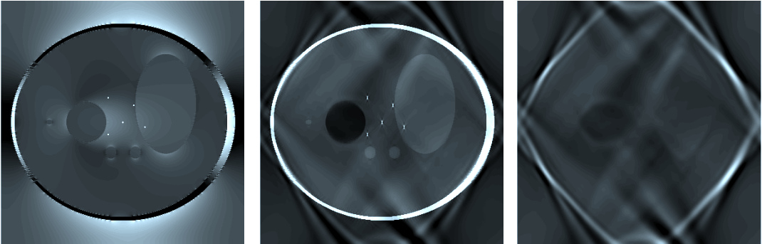
We can further reduce the order of the singularities as shown in figure 4 by increasing the order of the operator . More precisely, we consider
| (4.2) |
Moreover, for some smooth function such that , and , for some , we compute , where
| (4.3) |
with of symbol for some and (see figure 3(c)). The motivation behind the division of into two parts is that we would like to keep the smooth attributes of the image which are contained in , as well as reduce the artifacts included in . The images in figure 4 were obtained with , therefore the streaking artifacts are reduced to order while the other singularities to order .
Finally, by considering the operator defined in (3.3) and as in (4.2), the reconstructed susceptibility in figure 5 is computed by doing , where and
| (4.4) |
The streaking artifacts in are reduced by an order of while the rest of its singularities (the ones in ) remain in the same order when . By implementing this procedure the streaking artifacts are further reduced, in comparison with applying just TKD, and there is no attenuation of the rest of the singularities as for instance can be noticed in figure 6, which shows the part of the reconstructed susceptibilities that contains the streaking artifacts, this is , for the previous three cases.


References
- [1] J. K. Choi, H. S. Park, S. Wang, Y. Wang, J. K. Seo. Inverse Problem in Quantitative Susceptibility Mapping. SIAM Journal on Imaging Sciences, 7(3), 1669-1689, 2014.
- [2] J. J. Duistermaat. Fourier integral operators. Vol. 130. Springer Science & Business Media, 1996.
- [3] M. de Hoop, G. Uhlmann, A. Vasy. Diffraction from conormal singularities. Annales Scientifiques de l’École Normale Supérieure, 4e serie, t. 48, (2015): 351-408.
- [4] D. Finch, I. Lan, G. Uhlmann. Microlocal analysis of the X-ray transform with sources on a curve. Inside out: Inverse Problems and Applications 47 (2003): 193.
- [5] A. Greenleaf, G. Uhlmann. Nonlocal inversion formulas for the X-ray transform. Duke Math. J 58.1 (1989): 205-240.
- [6] A. Greenleaf, G. Uhlmann. Estimates for singular Radon transforms and pseudodifferential operators with singular symbols. Journal of Functional Analysis 89.1 (1990): 202-232.
- [7] A. Greenleaf, G. Uhlmann. Recovering singularities of a potential from singularities of scattering data. Communications in Mathematical Physics 157.3 (1993): 549-572.
- [8] A. Grigis, J. Sjöstrand. Microlocal analysis for differential operators: an introduction. Vol. 196. Cambridge University Press, 1994.
- [9] V. Guillemin, G. Uhlmann. Oscillatory integrals with singular symbols. Duke Math. J 48.1 (1981): 251-267.
- [10] L. Hörmander. The analysis of linear differential operators I. Grundlehren Math. Wiss 274 (1985).
- [11] L. Hörmander. The analysis of linear partial differential operators III: pseudo-differential operators. Classics in Mathematics, 2007.
- [12] L. Hörmander. The analysis of linear partial differential operators IV: Fourier integral operators. Classics in Mathematics, 2009.
- [13] Y. Kurylev, M. Lassas, G. Uhlmann. Seeing through spacetime. arXiv:1405.3386 (2014).
- [14] Y. Kurylev, M. Lassas, G. Uhlmann. Inverse problems in spacetime I: Inverse problems for Einstein equations-Extended preprint version. arXiv:1405.4503 (2014).
- [15] M. Lassas, G. Uhlmann, Y. Wang. Inverse problems for semilinear wave equations on Lorentzian manifolds. arXiv:1606.0626 (2016).
- [16] R. Melrose, G. Uhlmann. Lagrangian intersection and the Cauchy problem. Communications on Pure and Applied Mathematics 32.4 (1979): 483-519.
- [17] J. K. Seo, E. J. Woo, U. Katscher, Y. Wang. Electro-magnetic tissue properties MRI. Imperial College Press, Longdon, 2014.
- [18] Y. Wang. Principles of magnetic resonance imaging: physics concepts, pulse sequences, and biomedical applications. CreateSpace Independent Publishing Platform, 2012.