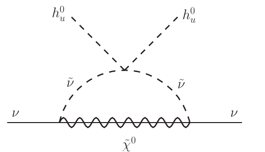
The coupling (6) is invariant under SM gauge symmetry. Since we are interested in neutrino mass generation, we extract from it the neutral components:

$$\lambda_{4}(\tilde{\nu}h_{u}^{0})^{2}+{\rm h.c.}$$

(8)

The combination $\tilde{\nu}\tilde{\nu}$ will be converted to $\nu\nu$ by the neutralino dressing diagram(s) shown in Fig. 1. The relevant terms are also

$$i\frac{g_{1}}{2}\tilde{B}\tilde{l}^{\dagger}l-i\frac{g_{2}}{\sqrt{2}}\tilde{W}_{b}^{a}\tilde{l_{a}}^{*}l^{b}+{\rm h.c.}\to\frac{i}{2}\nu\left(g_{1}\tilde{B}-g_{2}\tilde{W}^{0}\right)\tilde{\nu}^{*}+{\rm h.c.}$$

(9)

(given in 2-component notations of Ref. [11]) where $\tilde{B}$ and $\tilde{W}_{b}^{a}$ are $U(1)_{Y}$ and $SU(2)_{w}$ gauginos respectively. The indices $a,b=1,2$ belong to the $SU(2)_{w}$ gauge group. $\tilde{W}$’s matrix is defined as

$$\tilde{W}_{b}^{a}=\frac{1}{\sqrt{2}}\left(\!\!\!\begin{array}[]{cc}\tilde{W}^{0}&\sqrt{2}\tilde{W}^{+}\\ \sqrt{2}\tilde{W}^{-}&-\tilde{W}^{0}\\ \end{array}\!\!\right)^{\!\!a}_{\!\!b}~.$$

(10)

We are looking for the operator:

$$\frac{1}{2}\kappa^{\nu}_{ij}\nu_{i}\nu_{j}(h_{u}^{0})^{2}+{\rm h.c.}$$

(11)

where $\kappa^{\nu}_{ij}$ will be computed in terms of couplings appearing in (8), (9), together with other model parameters given below.

By diagonalization of $4\times 4$ neutralino mass matrix (of the states $\{-i\tilde{B},-i\tilde{W}^{0},\tilde{h}_{d}^{0},\tilde{h}_{u}^{0}\}$), the $\tilde{B}$ and $\tilde{W}^{0}$ get transformed as

$$\tilde{B}=U_{\!\chi 0}^{1\bar{a}}\hskip 1.42262pt\tilde{\chi}^{0}_{\bar{a}}~,\hskip 28.45274pt~~~~\tilde{W}^{0}=U_{\!\chi 0}^{2\bar{a}}\hskip 1.42262pt\tilde{\chi}^{0}_{\bar{a}}~,~~~~(\bar{a}=1,2,3,4)~,$$

(12)

where $\chi^{0}_{\bar{a}}$ is a physical mass eigenstate neutralino with mass $M_{\chi 0}^{\bar{a}}$. Using these in Eq. (9), the relevant couplings will be

$$\frac{i}{2}\nu\left(g_{1}U_{\!\chi 0}^{1\bar{a}}\hskip 1.42262pt-g_{2}U_{\!\chi 0}^{2\bar{a}}\hskip 1.42262pt\right)\chi^{0}_{\bar{a}}\tilde{\nu}^{*}+{\rm h.c.}$$

(13)

Interactions in Eqs. (8), (13) together with neutralino Majorana type mass terms, generate the operator of Eq. (11) via 1-loop diagram(s) shown in Fig. 1. Upon evaluation of the loop integral for the expression of $\kappa^{\nu}$ we obtain:

$$\kappa^{\nu}_{ij}=-\frac{\alpha_{2}}{8\pi}(\lambda_{4})_{ij}\sum_{\bar{a}=1}^{4}\frac{(\tan\theta_{W}U_{\!\chi 0}^{1\bar{a}}-U_{\!\chi 0}^{2\bar{a}})^{2}}{M_{\chi 0}^{\bar{a}}}f(x^{i}_{\bar{a}},x^{j}_{\bar{a}})~,$$

(14)

where $\tan\theta_{W}\!=\frac{g_{1}}{g_{2}}$ and

$$x^{i}_{\bar{a}}=\left(\!\frac{m_{\tilde{\nu}_{i}}}{M_{\chi 0}^{\bar{a}}}\!\right)^{\!\!2},~~~f(x_{1},x_{2})=\frac{x_{1}\ln x_{1}-x_{2}\ln x_{2}-x_{1}x_{2}\ln\frac{x_{1}}{x_{2}}}{(x_{1}-x_{2})(x_{1}-1)(x_{2}-1)}~.$$

(15)

From these expressions we can see that in order to have adequately suppressed neutrino masses($\stackrel{{\scriptstyle<}}{{{}_{\sim}}}0.1$ eV), for the SUSY particle masses$\sim$ TeV, we need to have $\lambda_{4}\stackrel{{\scriptstyle<}}{{{}_{\sim}}}10^{-8}$. In the next section we will see that this suppression can be naturally realized within presented models.

In this case, the MSSM is extended with right handed neutrino (RHN) superfields $N$. Since within our scenario, the masses of these states are near TeV scale, in order to avoid unacceptably large neutrino masses, we will need to suppress the $Y_{\nu}lNh_{u}$ type Yukawa superpotential couplings. Instead demanding ad hoc condition $|Y_{\nu}|\stackrel{{\scriptstyle<}}{{{}_{\sim}}}10^{-7}$, we will forbid such superpotential coupling by the $R$-symmetry, under which the superfield $\phi_{i}$ and the superpotential transform as:

$$\phi_{i}\to e^{iR_{i}}\phi_{i}~,~~~~~~~~W\to e^{i\omega}W~.$$

(16)

With the $R$ charge assignment for the superpotential $W$ and superfields $l,h_{u},N$ given in Table 1, together with the couplings $lNh_{u}$, also the $NN$-type superpotential terms are forbidden. However, as we will see shortly, the lepton number violating soft SUSY breaking terms will be induced. These type of terms will come from the Kähler potential, via the SUSY breaking. The latter will occur in a hidden sector with MSSM singlet superfield $X$ having non-zero $F$-term $F_{X}\sim m_{3/2}M_{Pl}$. The $R$ charge of the $X$ is selected to be $R_{X}=1$. In Table 1 we summarize $R$ charges of all superfields to be considered.

With this assignment, the following minimal and non-minimal Kähler (denoted below as ${\cal K}_{m}$ and ${\cal K}_{nm}$ respectively) potential couplings are allowed:

$${\cal K}_{m}=\sum_{f}f^{\dagger}e^{g_{a}V_{a}}f~,~~~{\cal K}_{nm}=\frac{X^{\dagger}}{2M_{\rm Pl}}\kappa NN+\frac{X^{\dagger}X}{\bar{M}^{3}}\kappa_{A}lNh_{u}+\frac{X^{\dagger}}{M_{\rm Pl}}\kappa_{h}h_{u}h_{d}+{\rm h.c.}$$

(17)

(On the second term in ${\cal K}_{nm}$, with cut off scale $\bar{M}<M_{\rm Pl}$, we comment below.) With these, the generated soft SUSY breaking terms involving $\tilde{N}$ will be:

$$V(\tilde{N})=\tilde{l}^{T}A_{N}\tilde{N}h_{u}+\frac{1}{2}\tilde{N}^{T}B_{N}\tilde{N}+{\rm h.c.}+\tilde{N}^{\dagger}M_{\tilde{N}}^{2}\tilde{N}~,$$

(18)

where $\tilde{l}^{T}=(\tilde{l}_{1},\tilde{l}_{2},\tilde{l}_{3})$ and $\tilde{N}^{T}=(\tilde{N}_{1},\tilde{N}_{2},\cdots)$ (the number of $\tilde{N}$ states should be $\geq 2$). The matrix $M_{\tilde{N}}^{2}$ is hermitian while $B_{N}$ is a symmetric: $M_{\tilde{N}}^{2}=(M_{\tilde{N}}^{2})^{\dagger}$ and $B_{N}^{T}=B_{N}$. The mass² terms in (18) with $F_{X}\sim m_{3/2}M_{\rm Pl}$ are $M_{\tilde{N}}^{2}\sim|F_{X}|^{2}/M_{\rm Pl}^{2}\sim m_{3/2}^{2}$. The soft $B$-terms are $B_{N}\sim\kappa|F_{X}|^{2}/M_{\rm Pl}^{2}\sim\kappa m_{3/2}^{2}$, while with $\bar{M}\sim(m_{3/2}M_{Pl}^{2})^{1/3}$ the trilinear $A$-term will be $A_{N}\sim\kappa_{A}|F_{X}|^{2}/\bar{M}^{3}\sim\kappa_{A}m_{3/2}$. For detailed discussion and derivations see Appendix A. In the same Appendix we discuss the generation of $F_{X}$ via Polonyi superpotential and specific Kähler potential for $X$.

From the couplings in Eq. (18), by integrating out the $\tilde{N}$ states we get the operator of Eq. (6). In particular, by assumption $\kappa\stackrel{{\scriptstyle<}}{{{}_{\sim}}}1/3,\kappa_{A}v_{u}\stackrel{{\scriptstyle<}}{{{}_{\sim}}}0.3m_{3/2}$, the expression for $\lambda_{4}$ can be approximated as:

$$\lambda_{4}\simeq\frac{1}{2}A_{N}\frac{1}{M_{\tilde{N}}^{2}}B_{N}^{\dagger}\frac{1}{(M_{\tilde{N}}^{2})^{T}}A_{N}^{T}~.$$

(19)

Corresponding diagram is given in Fig. 2. Derivation and more accurate expression for $\lambda_{4}$ is given in Appendix B by Eq. (B.7). From the structure of (19) and process given in Fig. 2 it is clear why it is fair to call this mechanism (for generating of $\lambda_{4}$ coupling) the type I soft see-saw. The quartic operator of (6) is forbidden in the SUSY limit, but is generated due to SUSY breaking $\Delta L=2$ terms via integrating out the $\tilde{N}$ states. With these, as was shown in section 2.1, the neutrino masses are generated at 1-loop level. The needed suppression for the $\lambda_{4}$ is easily obtained. For instance, with the SUSY particle masses $\sim$ few TeV and $\frac{A_{N}}{M_{\tilde{N}}}\sim\frac{\sqrt{B_{N}}}{M_{\tilde{N}}}\sim 10^{-2}$, from (19) we can get $\lambda_{4}\sim 10^{-8}$ - guaranteeing suppressed values of the neutrino masses($\sim 0.1$ eV).

The second operator in ${\cal K}_{nm}$ of Eq. (17) can be obtained by integrating some heavy states. Here we give one example. By introducing additional MSSM singlet states ${\cal N},\overline{\cal N},{\cal N}^{\prime}$ and $\overline{\cal N}^{\prime}$ we can have the Kähler coupling ${\cal K}_{{\cal N}}=\frac{\kappa_{{\cal N}}X^{\dagger}}{M_{Pl}}N\overline{\cal N}$ and the superpotential terms: $W_{{\cal N}}=M_{{\cal N}}{\cal N}\overline{\cal N}+\lambda_{X}X{\cal N}\overline{\cal N}^{\prime}+{M^{\prime}}_{{\cal N}}{\cal N}^{\prime}\overline{\cal N}^{\prime}+\lambda_{{\cal N}}\overline{\cal N}^{\prime}lh_{u}$. One can easily verify that integration of the states ${\cal N},\overline{\cal N},{\cal N}^{\prime},\overline{\cal N}^{\prime}$ induces the Kähler operator $\frac{\kappa_{{\cal N}}\lambda_{X}\lambda_{{\cal N}}}{M_{Pl}M_{{\cal N}}{M^{\prime}}_{{\cal N}}}X^{\dagger}XlNh_{u}$. Comparing this with Eq. (17), one can identify $\frac{k_{A}}{\bar{M}^{3}}=\frac{\kappa_{{\cal N}}\lambda_{X}\lambda_{{\cal N}}}{M_{Pl}M_{{\cal N}}{M^{\prime}}_{{\cal N}}}$.

As shown in Appendix A, by the construction one can insure that the VEV of the $X$ field can be adequately suppressed. With $\langle X\rangle\stackrel{{\scriptstyle<}}{{{}_{\sim}}}10^{-7}M_{Pl}$ the neutrino Dirac Yukawa couplings, generated via the Kähler potential will be $Y_{\nu}\stackrel{{\scriptstyle<}}{{{}_{\sim}}}10^{-7}$ (see expression in (A.23) and related discussion before and after of this equation), i.e. not relevant for the neutrino masses. On the other hand, there is a low bound on the values of $Y_{\nu}$ couplings. They should be sizable enough to insure decays of the fermionic RHN states $N$ within $\stackrel{{\scriptstyle<}}{{{}_{\sim}}}0.3$ sec. in order to not affect the standard Big Bang nucleosynthesis. With $M_{N}>M_{l}+M_{h_{u}}(M_{\tilde{l}}+M_{\tilde{h}})$ we will have decays $N\to lh_{u}(\tilde{l}\tilde{h})$, with the lifetime given by

$$\Gamma_{N\to lh_{u}(\tilde{l}\tilde{h})}^{-1}\approx\frac{8\pi}{|Y_{\nu}|^{2}M_{N}}=0.3~{\rm sec.}\times\left(\frac{2.34\cdot 10^{-13}}{|Y_{\nu}|}\right)^{2}\left(\frac{1~{\rm TeV}}{M_{N}}\right).$$

(20)

Since $Y_{\nu}\sim\langle X\rangle/M_{Pl}$, we will have the low bound on the VEV $\langle X\rangle\stackrel{{\scriptstyle>}}{{{}_{\sim}}}5.6\cdot 10^{5}$ GeV. Therefore, summarizing all above, we will have the following range:

$$2.34\cdot 10^{-13}\stackrel{{\scriptstyle<}}{{{}_{\sim}}}Y_{\nu}\stackrel{{\scriptstyle<}}{{{}_{\sim}}}10^{-7}~~~~\longrightarrow~~~~5.6\cdot 10^{5}~{\rm GeV}\stackrel{{\scriptstyle<}}{{{}_{\sim}}}\langle X\rangle\stackrel{{\scriptstyle<}}{{{}_{\sim}}}2\cdot 10^{11}~{\rm GeV}.$$

(21)

The mass $M_{N}$ is generated from the first coupling of ${\cal K}_{nm}$ of (17), with the value $M_{N}\sim\kappa F_{X}/M_{\rm Pl}\sim\kappa m_{3/2}$. Note that, it is easy to satisfy $M_{N}>M_{l}+M_{h_{u}}(M_{\tilde{l}}+M_{\tilde{h}})$ insuring the decays described in (20).

Closing this subsection, with the $R$-charge assignment given in Table 1, the MSSM Yukawa superpotential couplings are:

$$W_{Y}^{MSSM}=Y_{U}qu^{c}h_{u}+Y_{D}qd^{c}h_{d}+Y_{E}le^{c}h_{d}~.$$

(22)

Note that the direct $h_{u}h_{d}$ superpotential term is forbidden. However, as shown first in Ref. [12], the last coupling in (17) generates $\mu\sim\kappa_{h}m_{3/2}$ and $B\mu\sim\kappa_{h}m_{3/2}^{2}$ terms.

With the $R$-charge assignments given in Table 1 the lepton number violating superpotential couplings $X^{n}h_{u}l$ (which break also matter parity) are all forbidden for $\omega\neq m+1/2$ (where $m$ is an integer). Also the trilinear lepton number violating interactions $qd^{c}l$ and $e^{c}ll$ will be forbidden in the superpotential. The baryon number violating term $u^{c}d^{c}d^{c}$ can be forbidden if the phases $\alpha_{q}$, $\omega$ and $\alpha$ will satisfy additional condition $3\alpha_{q}-2\omega-\alpha\neq m_{1}$ ($m_{1}\in Z$). With these and with one more condition $3\alpha_{q}-\omega-\alpha\neq m_{2}$ ($m_{2}\in Z$) the $d=5$ baryon and lepton number violating couplings $qqql$, $u^{c}u^{c}d^{c}e^{c}$ and $qqqh_{d}$ will be automatically forbidden. One can also make sure that with these three conditions

$$\omega\neq m+1/2~,~~~3\alpha_{q}-2\omega-\alpha\neq m_{1}~,~~~3\alpha_{q}-\omega-\alpha\neq m_{2}~~~~~(m,m_{1,2}\in Z)~,$$

(23)

baryon and matter parity violating couplings do not emerge also from the Kähler potential.

In this case we extend the MSSM by introducing the pair of $SU(2)_{w}$ triplet and antitriplet superfields $\Sigma$, $\bar{\Sigma}$ with $U(1)_{Y}$ hypercharges $2$ and $-2$ respectively (in this normalization, the hypercharge of the lepton doublet $l=(e^{-},\nu)$ equals to $-1$). $\Sigma$ and $\bar{\Sigma}$ are $2\times 2$ matrices in $SU(2)_{w}$ space and their compositions are given by:

$$\Sigma_{ab}\!=\!\left(\begin{array}[]{cc}\Sigma^{(++)}&\Sigma^{(+)}/\sqrt{2}\\ \Sigma^{(+)}/\sqrt{2}&\Sigma^{(0)}\\ \end{array}\right)_{\!\!ab}~,~~~~\bar{\Sigma}^{ab}\!=\!\left(\begin{array}[]{cc}\bar{\Sigma}^{(--)}&\bar{\Sigma}^{(-)}/\sqrt{2}\\ \bar{\Sigma}^{(-)}/\sqrt{2}&\bar{\Sigma}^{(0)}\\ \end{array}\right)^{\!\!ab}~,~$$

(24)

where signs in superscripts indicate electric charges [e.g. $(++)$ stands with the double charged state].

With this field content, two scenarios which somewhat differ from each other, can be considered. We refer to them as type II-A soft and type II-B soft see-saw models.

Type II-A soft see-saw model

In this case, the $R$-charge assignment is given in Table 2

and relevant Kähler potential couplings are:

$${\cal K}_{m}=\sum_{f}f^{\dagger}e^{g_{a}V_{a}}f~,~~~{\cal K}_{nm}=\frac{\kappa}{M_{\rm Pl}}X^{\dagger}\bar{\Sigma}\Sigma+\frac{X^{\dagger}X}{\bar{M}^{3}}\!\left(\!\kappa_{A\bar{\Sigma}}\bar{\Sigma}h_{u}h_{u}+\frac{1}{2}\kappa_{A\Sigma}\Sigma ll\right)\!+\frac{\kappa_{h}}{M_{\rm Pl}}X^{\dagger}h_{u}h_{d}+{\rm h.c.}$$

(25)

The MSSM superpotential couplings will be same as given in (22). The couplings of Eq. (25) and SUSY breaking hidden sector, together with the $\mu$ and $B$-terms for the MSSM Higgs doublets, generate the following soft terms involving the scalar components of $\Sigma$ and $\bar{\Sigma}$:

$$V(\Sigma,\bar{\Sigma})=B_{\Sigma}\bar{\Sigma}\Sigma+A_{\bar{\Sigma}}\bar{\Sigma}h_{u}h_{u}+\Sigma\hskip 1.13809pt\tilde{l}^{\hskip 1.13809ptT}A_{\Sigma}\tilde{l}+{\rm h.c}+M_{\Sigma}^{2}\Sigma^{\dagger}\Sigma+M_{\bar{\Sigma}}^{2}\bar{\Sigma}^{\dagger}\bar{\Sigma}~.$$

(26)

Here $\Sigma$ and $\bar{\Sigma}$ denote bosonic components. Their fermionic partners will be denoted by $\tilde{\Sigma}$ and $\tilde{\bar{\Sigma}}$ respectively. Integration of $\Sigma,\bar{\Sigma}$ states leads to the operator of Eq. (6) with approximate expression for $\lambda_{4}$ given by:

$$\lambda_{4}\simeq\frac{1}{M_{\Sigma}^{2}M_{\bar{\Sigma}}^{2}}A_{\bar{\Sigma}}B_{\Sigma}^{*}A_{\Sigma}~,$$

(27)

valid for $M_{\Sigma}M_{\bar{\Sigma}}\stackrel{{\scriptstyle>}}{{{}_{\sim}}}|B_{\Sigma}|/3$. More accurate expression is given in Appendix B [see Eq. (B.10)]. The first diagram of Fig. 3 corresponds to the generation of this operator, which gives loop induced neutrino masses as shown in Sect. 2.1. Also within this case, the needed suppression of $\lambda_{4}$ can be achieved, for example, by the selection $\frac{A_{\Sigma}}{M_{\Sigma}}\sim\frac{A_{\bar{\Sigma}}}{M_{\Sigma}}\sim\frac{\sqrt{B_{\Sigma}}}{M_{\bar{\Sigma}}}\sim 10^{-2}$.

Via exchange of $\Sigma,\bar{\Sigma}$ states, the four slepton interaction operator is also generated, which in the same approximation (as Eq. (27)) is:

$${\cal L}_{4\tilde{l}}^{\rm eff}=\frac{1}{M_{\Sigma}^{2}}\left(\tilde{l}^{\hskip 1.13809ptT}_{a}A_{\Sigma}\tilde{l}_{b}\right)\left(\tilde{l}^{\hskip 1.13809pt{\dagger}}_{a}A_{\Sigma}^{*}\tilde{l}^{\hskip 0.85358pt*}_{b}\right),$$

(28)

where $a,b=1,2$ are $SU(2)_{w}$ indices [see Eq. (B.11) for more accurate expression]. The corresponding diagram is the second one in Fig. 3.

By 2-loop gaugino/higgsino dressing diagrams, the operator (28) will be converted to the four lepton operator $C^{4l}_{ijmn}(l^{i}_{a}l^{j}_{b})(\bar{l}^{m}_{a}\bar{l}^{n}_{b})$. One relevant diagram is shown in Fig. 4. These couplings (i.e. $C^{4l}_{ijmn}$) in turn induce $e_{i}\to e_{j}e_{m}e_{n}$ rare decays, including processes such as $\tau\to 3\mu$, $\mu\to 3e$ etc. With all SUSY particles and $\Sigma,\bar{\Sigma}$ states having the common masses$\approx M_{S}$ we estimate $C^{4l}_{ijmn}\approx\left(\frac{\alpha_{2}}{4\pi}\right)^{2}\frac{(A_{\Sigma})_{ij}(A_{\Sigma}^{*})_{mn}}{M_{S}^{4}}$. For instance, for the branching ratio of the reaction $\mu\to 3e$ we will have

$${Br}(\mu\to 3e)\approx\left(\frac{\alpha_{2}}{4\pi}\right)^{4}\frac{|(A_{\Sigma})_{11}(A_{\Sigma}^{*})_{12}|^{2}}{G_{F}^{2}M_{S}^{8}}\simeq 3.8\cdot 10^{-13}\left(\frac{1~{\rm TeV}}{M_{S}}\right)^{4}\left|\frac{(A_{\Sigma})_{11}(A_{\Sigma}^{*})_{12}}{M_{S}^{2}}\right|^{2}~.$$

(29)

We see that with $M_{S}\sim 1$ TeV, the current experimental limit ${Br}(\mu\to 3e)<10^{-12}$ [13] is easily satisfied even with $\frac{(A_{\Sigma})_{11}}{M_{S}},\frac{(A_{\Sigma})_{12}}{M_{S}}\sim 1$. If the latter ratios are taken to be suppressed, then one can allow to have $M_{S}$’s values below the TeV scale. Since the experimental limits on $\tau$’s rare decays are less stringent [13], it is easier to satisfy bounds on branching ratios $Br(\tau\to e_{i}e_{j}e_{k})$. Since $A_{\Sigma}$ couplings also enter in the neutrino mass matrix [see Eq. (27)], it would be interesting to investigate their flavor structure in connection to the neutrino data and the rare lepton decays. These will open window to probe the neutrino mass generation mechanism presented here.

Finally, the $\kappa$-term in Eq. (25) generates the mass term for the fermionic $\tilde{\Sigma},\tilde{\bar{\Sigma}}$ components $\mu_{\Sigma}\tilde{\bar{\Sigma}}\tilde{\Sigma}$ with $\mu_{\Sigma}\sim\kappa m_{3/2}$.

Type II-B soft see-saw model

In this modified version, the neutrino masses are induced at 2-loop level. The $R$-charges of the states are given in Table 3

and the Kähler potential couplings are

$${\cal K}_{m}=\sum_{f}f^{\dagger}e^{g_{a}V_{a}}f~,~~~{\cal K}_{nm}=\frac{\kappa}{M_{\rm Pl}}X^{\dagger}\bar{\Sigma}\Sigma+\frac{X^{\dagger}X}{2\bar{M}^{3}}\kappa_{A\Sigma}\Sigma\hskip 1.13809ptll\!+\frac{\kappa_{h}}{M_{\rm Pl}}X^{\dagger}h_{u}h_{d}+{\rm h.c.}$$

(30)

The $X^{\dagger}\bar{\Sigma}h_{u}h_{u}$ term is forbidden in the Kähler potential, but the following superpotential coupling, involving $\bar{\Sigma}$, is allowed:

$$W_{\bar{\Sigma}}=\lambda_{\bar{\Sigma}}\bar{\Sigma}h_{u}h_{u}~.$$

(31)

The MSSM superpotential terms are same as given in Eq. (22).

The coupling (31), in general would generate the trilinear soft term $A_{\bar{\Sigma}}\bar{\Sigma}h_{u}h_{u}$. However, within the SUSY breaking scenario we are considering, this $A$-term is suppressed:

$$A_{\bar{\Sigma}}\sim\lambda_{\bar{\Sigma}}m_{3/2}\frac{\langle X\rangle}{M_{Pl}}\stackrel{{\scriptstyle<}}{{{}_{\sim}}}10^{-7}\lambda_{\bar{\Sigma}}m_{3/2}~.$$

(32)

(see Eq. (A.25) and discussion therein).

Kähler potential terms of Eq. (30), besides higgsino $\mu$ and Higgs $B$ terms induce the potential terms:

$$B_{\Sigma}\bar{\Sigma}\Sigma+A_{\Sigma}\Sigma\tilde{l}\tilde{l}+{\rm h.c}+M_{\Sigma}^{2}\Sigma^{\dagger}\Sigma+M_{\bar{\Sigma}}^{2}\bar{\Sigma}^{\dagger}\bar{\Sigma}~.$$

(33)

With the couplings in (32), (33), integration of $\Sigma,\bar{\Sigma}$ states leads to the operator of Eq. (6) with expression for $\lambda_{4}$ having the same form as given in Eq. (27), but with extra strong suppression factor$\stackrel{{\scriptstyle<}}{{{}_{\sim}}}10^{-7}$. Therefore, 1-loop contribution to the neutrino masses will be very suppressed and can be ignored. Neutrino masses will be induced at 2-loop level, which we discuss below.

The superpotential of Eq. (31) gives the following Yukawa interactions:

$$\int d^{2}\theta W_{\bar{\Sigma}}\to\lambda_{\bar{\Sigma}}\left(\bar{\Sigma}\tilde{h}_{u}\tilde{h}_{u}+2\tilde{\bar{\Sigma}}\tilde{h}_{u}h_{u}\right)~.$$

(34)

These couplings, together with those given in (33), upon integration of scalar components from ${\bar{\Sigma}},\Sigma$ superfields, induce the following $\Delta L=2$ dimension $5$ operator ($\lambda_{5}^{\prime}$-type of Eq. (5)):

$$\lambda_{5}^{\prime}(\tilde{l}\hskip 1.42262pt\tilde{h}_{u})^{2}~,~~~~{\rm with}~~~~\lambda_{5}^{\prime}\simeq\frac{1}{M_{\Sigma}^{2}M_{\bar{\Sigma}}^{2}}\lambda_{\bar{\Sigma}}B_{\Sigma}^{*}A_{\Sigma}~.$$

(35)

The way of derivation of this $d=5$ operator is similar to that given in Appendix B. We just need to make replacement $A_{\bar{\Sigma}}h_{u}h_{u}\to\lambda_{\bar{\Sigma}}\tilde{h}_{u}\tilde{h}_{u}$ in Eq. (B.10). The operator (35), by the gaugino dressings at 2-loop gives the $d=5$ operator $\lambda_{5}(l\hskip 1.42262pth_{u})^{2}$ responsible for the neutrino mass. The relevant diagrams are given in Fig. 5. For consistency, one should also take into account the effective $d=6$, $\Delta L=2$ operators

$$-\frac{2}{M_{\Sigma}^{2}\mu_{\Sigma}}\lambda_{\bar{\Sigma}}(\tilde{l}^{\hskip 1.13809ptT}A_{\Sigma}\tilde{l})(g\tilde{V}\tilde{h}_{u}h_{u})+{\rm h.c.}$$

(36)

(the $\lambda_{6}^{\prime}$-type coupling of Eq. (7)) which are induced by integration of the scalar and fermionic components from ${\bar{\Sigma}},\Sigma$ superfields [by using the mass term $\mu_{\Sigma}\tilde{\bar{\Sigma}}\tilde{\Sigma}$ and couplings (33), (34)]. In (36), $g\tilde{V}=\{g_{1}\tilde{B},g_{2}\tilde{W}\}$ denote $U(1)_{Y}$ and/or $SU(2)_{w}$ gaugino contributions.

Care must be taken to treat properly divergences of the diagrams in Fig. 5. If the effective vortexes (35) and (36) are used without specifying the model (the operators are induced from), the loops need to be cut off by the characteristic scale. Since within type II soft see-saw, these operators are obtained by integrating $\Sigma,\bar{\Sigma}$ states, full calculation can be done. With ’opening’ vortexes, the diagrams are shown in Fig. 6.

It is obvious that log divergence of the first and third diagrams are coming from upper triangles corresponding to the parts of one loop renormalization of the soft $A_{\bar{\Sigma}}$ term (vanishing at tree level). Indeed,

$$\delta A_{\bar{\Sigma}}=\delta A_{\bar{\Sigma}}^{(1)}+\delta A_{\bar{\Sigma}}^{(2)}~,~~~~~{\rm with}$$

$$\delta A_{\bar{\Sigma}}^{(1)}=-\frac{\lambda_{\bar{\Sigma}}}{16\pi^{2}}\!\sum_{a=1}^{3}\!c^{(1)}_{a}g^{2}_{a}M_{\tilde{V}_{a}}\!\!\left(\!\ln\frac{\Lambda^{2}}{M_{\tilde{V}_{a}}^{2}}+\frac{\mu^{2}(2M_{\tilde{V}_{a}}^{2}-\mu^{2})}{(M_{\tilde{V}_{a}}^{2}-\mu^{2})^{2}}\ln\frac{\mu^{2}}{M_{\tilde{V}_{a}}^{2}}-\frac{\mu^{2}}{\mu^{2}-M_{\tilde{V}_{a}}^{2}}\!\right),$$

$$\delta A_{\bar{\Sigma}}^{(2)}=-\frac{\lambda_{\bar{\Sigma}}}{16\pi^{2}}\!\sum_{a=1}^{3}\!c^{(2)}_{a}g^{2}_{a}M_{\tilde{V}_{a}}\!\!\left(\!\ln\frac{\Lambda^{2}}{M_{\tilde{V}_{a}}^{2}}-\frac{\mu^{4}\ln\frac{\mu^{2}}{M_{\tilde{V}_{a}}^{2}}}{(\mu^{2}-\mu_{\Sigma}^{2})(\mu^{2}-M_{\tilde{V}_{a}}^{2})}-\frac{\mu_{\Sigma}^{4}\ln\frac{\mu_{\Sigma}^{2}}{M_{\tilde{V}_{a}}^{2}}}{(\mu_{\Sigma}^{2}-\mu^{2})(\mu_{\Sigma}^{2}-M_{\tilde{V}_{a}}^{2})}\!\right),$$

$${\rm with}~~~~~~c^{(1)}_{a}=\left(\frac{6}{5},3,0\right),~~~~c^{(2)}_{a}=\left(\frac{3}{5},6,0\right),$$

(37)

where $\mu$ and $\mu_{\Sigma}$ are the MSSM higgsino $\mu$-term and the mass of the fermionic $\tilde{\Sigma},\tilde{\bar{\Sigma}}$ states respectively, $g_{a}$ is the gauge coupling (with $c_{a}^{(1,2)}$ being corresponding group theoretical factors and $M_{\tilde{V}_{a}}$ the corresponding gaugino’s soft mass). In the last line of (37), $a=1,2,3$ labels $U(1)_{Y}$, $SU(2)_{w}$ and $SU(3)_{c}$ gauge groups respectively (the coupling $g_{1}$ is taken in $SU(5)$ normalization). The $\ln\Lambda$ terms coincide with those obtained via integration of the RG equation for the $A_{\bar{\Sigma}}$ soft term. Expressions (37), after the renormalization, leave us with a non-divergent and finite parts. Assuming the boundary condition $A_{\bar{\Sigma}}(M_{UV})=0$ at some scale $M_{UV}$ (which can be the Planck mass, in case of gravity mediated SUSY breaking), at the SUSY scale $M_{S}$, we will have:

$${\rm at}~~~~\mu=M_{S}:~~~~~~~A_{\bar{\Sigma}}^{\rm eff}=-\frac{\lambda_{\bar{\Sigma}}}{16\pi^{2}}\!\left(\!\sum_{a=1}^{3}\!c_{a}g^{2}_{a}M_{\tilde{V}_{a}}\!\right)\!\ln\frac{M_{UV}^{2}}{M_{S}^{2}},~~~~c_{a}=\left(\frac{9}{5},9,0\right).$$

(38)

Further, we compute the lower triangle diagrams of Fig. 6-(a),(c), which by the gaugino dressings convert $\tilde{l}\tilde{l}$ to $ll$. Then, integrate out the $\Sigma,\bar{\Sigma}$ states and obtain the contribution to the neutrino mass to be given by:⁷⁷ 7 Here we ignore the EW symmetry breaking effects, e.g. the gaugino-higgsino mixings.

$$\left(\delta M_{\nu}^{ij}\right)_{\rm Fig.5-(a)+(c)}=\frac{v_{u}^{2}A_{\bar{\Sigma}}^{\rm eff}}{16\pi^{2}}\frac{B_{\Sigma}^{*}A_{\Sigma}^{ij}}{M^{2}_{\Sigma}M^{2}_{\bar{\Sigma}}}\sum_{a=1}^{3}\!\frac{c^{(1)}_{a}g^{2}_{a}}{M_{\tilde{V}_{a}}}f\!\left[\!\left(\!\frac{m_{i}}{M_{\tilde{V}_{a}}}\!\right)^{2}\!\!\!,\left(\!\frac{m_{j}}{M_{\tilde{V}_{a}}}\!\right)^{2}\right]~,$$

(39)

where the function $f$ is defined in Eq. (15) and $m_{i},m_{j}$ denote masses of $\tilde{l}_{i},\tilde{l}_{j}$.

References

- [1] G. L. Fogli, E. Lisi, A. Marrone, D. Montanino, A. Palazzo and A. M. Rotunno, Phys. Rev. D 86 (2012) 013012; M. C. Gonzalez-Garcia, M. Maltoni and T. Schwetz, JHEP 1411 (2014) 052.
- [2] P. Minkowski, Phys. Lett. B 67 (1977) 421; M. Gell-Mann, P. Ramond and R. Slansky, Conf. Proc. C 790927 (1979) 315; T. Yanagida, Conf. Proc. C 7902131 (1979) 95; S. L. Glashow, NATO Sci. Ser. B 61 (1980) 687; R. N. Mohapatra and G. Senjanovic, Phys. Rev. Lett. 44 (1980) 912; J. Schechter and J. W. F. Valle, Phys. Rev. D 25 (1982) 774.
- [3] M. Magg and C. Wetterich, Phys. Lett. B 94 (1980) 61; J. Schechter and J. W. F. Valle, Phys. Rev. D 22 (1980) 2227; T. P. Cheng and L. F. Li, Phys. Rev. D 22 (1980) 2860; G. Lazarides, Q. Shafi and C. Wetterich, Nucl. Phys. B 181 (1981) 287; R. N. Mohapatra and G. Senjanovic, Phys. Rev. D 23 (1981) 165.
- [4] R. Foot, H. Lew, X. G. He and G. C. Joshi, Z. Phys. C 44 (1989) 441; E. Ma, Phys. Rev. Lett. 81 (1998) 1171.
- [5] S. Weinberg, Phys. Rev. Lett. 43 (1979) 1566; Phys. Rev. D 22 (1980) 1694.
- [6]
A. Zee,
Phys. Lett. B 93 (1980) 389;
Nucl. Phys. B 264 (1986) 99;
K. S. Babu, Phys. Lett. B 203 (1988) 132. - [7] A. Pilaftsis, Z. Phys. C 55 (1992) 275; K. S. Babu and J. Julio, Nucl. Phys. B 841 (2010) 130; Phys. Rev. D 85 (2012) 073005.
- [8] E. Ma, Phys. Rev. D 73 (2006) 077301.
- [9] P. S. B. Dev and A. Pilaftsis, Phys. Rev. D 86 (2012) 113001; S. Fraser, E. Ma and O. Popov, Phys. Lett. B 737 (2014) 280; S. Fraser, C. Kownacki, E. Ma and O. Popov, Phys. Rev. D 93 (2016) no.1, 013021; For a recent work and exhaustive list of references see: T. Nomura and H. Okada, arXiv:1609.01504 [hep-ph].
- [10] Y. Grossman and H. E. Haber, Phys. Rev. Lett. 78 (1997) 3438; N. Arkani-Hamed, L. J. Hall, H. Murayama, D. Tucker-Smith and N. Weiner, hep-ph/0007001; F. Borzumati and Y. Nomura, Phys. Rev. D 64 (2001) 053005; J. March-Russell and S. M. West, Phys. Lett. B 593 (2004) 181.
- [11] J. Wess and J. Bagger, “Supersymmetry and supergravity,” Princeton, USA: Univ. Pr. (1992) 259 pp.
- [12] G. F. Giudice and A. Masiero, Phys. Lett. B 206 (1988) 480.
- [13] J. Beringer et al. [Particle Data Group Collaboration], “Review of Particle Physics (RPP),” Phys. Rev. D 86 (2012) 010001.
- [14] B. Bajc, M. Nemevsek and G. Senjanovic, Phys. Rev. D 76 (2007) 055011; A. G. Akeroyd, M. Aoki and H. Sugiyama, Phys. Rev. D 77 (2008) 075010; P. Fileviez Perez, T. Han, G. y. Huang, T. Li and K. Wang, Phys. Rev. D 78 (2008) 015018. S. M. Boucenna, S. Morisi and J. W. F. Valle, Adv. High Energy Phys. 2014 (2014) 831598.
- [15] K. S. Babu, S. Nandi and Z. Tavartkiladze, Phys. Rev. D 80 (2009) 071702.
- [16] Z. Tavartkiladze, Phys. Lett. B 528 (2002) 97; Z. z. Xing and S. Zhou, Phys. Lett. B 679 (2009) 249; F. Bonnet, D. Hernandez, T. Ota and W. Winter, JHEP 0910 (2009) 076; S. Kanemura and T. Ota, Phys. Lett. B 694 (2011) 233; K. Kumericki, I. Picek and B. Radovcic, Phys. Rev. D 86 (2012) 013006; P. W. Angel, N. L. Rodd and R. R. Volkas, Phys. Rev. D 87 (2013) no.7, 073007; and references therein.
- [17]
S. Ferrara, M. Kaku, P.K. Townsend, P. van Nieuwenhuizen,
Nucl. Phys. B 129 (1977) 125;
M. Kaku, P. K. Townsend and P. van Nieuwenhuizen, Phys. Rev. D 17 (1978) 3179;
E. Cremmer, B. Julia, J. Scherk, S. Ferrara, L. Girardello and P. van Nieuwenhuizen, Nucl. Phys. B 147 (1979) 105. - [18] T. Kugo and S. Uehara, Nucl. Phys. B 222 (1983) 125; V. Kaplunovsky and J. Louis, Nucl. Phys. B 422 (1994) 57.
- [19] J. Polonyi, Hungary Central Inst Res - KFKI-77-93 (77,REC.JUL 78) 5p.
- [20] A. E. Nelson and N. Seiberg, Nucl. Phys. B 416 (1994) 46.
- [21] D.Z. Freedman and A. Van Proeyen, “Supergravity,” Cambridge, Univ. Pr. (2012) 607 pp.
- [22] A. Brignole, Nucl. Phys. B 579 (2000) 101.