On the Late-Time Behavior of Virasoro Blocks
and a Classification of Semiclassical Saddles

Although any violation of unitarity in quantum gravity might be construed as ‘information loss’, we would like to be more specific and zero in on information loss associated with black holes. In this work we will focus on physical processes where initial data disappears because a high-energy microstate behaves too much like the thermal ensemble, i.e. as if the heavy state is a perfect thermal bath with an infinite number of degrees of freedom. This seems to be a good description of why encyclopedias are destroyed when they fall into semiclassical black holes.

The information loss problem(s) we will discuss can be studied by observers who stay far away from a black hole, meaning that in the AdS/CFT context, the problem can be diagnosed using only CFT correlators [13], without reconstructing the AdS spacetime. Thus we are studying the ‘easier’ information loss problem [11], rather than the ‘hard’ problem of how to simultaneously maintain unitarity and effective field theory across the horizon of a black hole. From the point of view of CFT the problem has two parts: first we must understand why the CFT appears non-unitary at large $c$, and then, from this vantage point, we need to identify the effects that restore the information.

We will be focusing on 4-point correlators in CFT₂, which we will write as

$\displaystyle\langle{\cal O}_{H}(\infty){\cal O}_{H}(1){\cal O}_{L}(z){\cal O}_{L}(0)\rangle$

(1.1)

to emphasize that we are most interested in the physics of the heavy-light limit where a relatively light probe interacts with a black hole in AdS₃. The dual AdS₃ setup is pictured in figure 1. The ratios $\frac{h_{i}}{c}\sim G_{N}M_{i}$ are fixed in the semiclassical large $c$ limit. In this paper, unlike in many of our previous works, we will obtain results that hold for arbitrary values of both $\frac{h_{L}}{c}$ and $\frac{h_{H}}{c}$. Our methods will pertain to the entire semiclassical regime.

We recently discussed two sharp signatures of information loss [11] encoded in the heavy-light CFT correlator, ‘forbidden singularities’ and the late time behavior [13] of the correlator. Here we will be focusing on the latter.

If we consider a schematic decomposition of the heavy-light correlator in the ${\cal O}_{H}{\cal O}_{L}\to{\cal O}_{H}{\cal O}_{L}$ OPE channel, which corresponds to conventional time slices of the cylinder pictured in figure 1, we find

$\displaystyle\langle{\cal O}_{H}(\infty){\cal O}_{L}(t){\cal O}_{L}(0){\cal O}_{H}(-\infty)\rangle=\sum_{i}\lambda_{i}e^{iE_{i}t}$

(1.2)

for some coefficients $\lambda_{i}$ and energy levels $E_{i}$. In the presence of a large number of terms, well-known statistical considerations apply (see [14] for a relevant, detailed discussion). In holographic CFTs, these suggest that the correlator will decay exponentially until it is of order $e^{-\frac{1}{2}S_{BH}}$, where $S_{BH}$ is the heavy-state black hole entropy. After this point it enters a chaotic phase where it is typically very small, but occassionally returns to an order one value due to Poincaré recurrences on timescales of order $e^{S_{BH}}$. This channel seems to describe healthy unitary evolution as long as the $\lambda_{i}$ are discrete and finite, and in particular it is hard to see how information loss can occur. Individual unitary conformal blocks in this channel bear little resemblance to the physics of semiclassical gravity, which produces a continuous spectrum in the limit $c\rightarrow\infty$ [1].

We will be focusing instead on the ${\cal O}_{L}{\cal O}_{L}\to{\cal O}_{H}{\cal O}_{H}$ OPE channel

$\displaystyle\langle{\cal O}_{H}(\infty){\cal O}_{L}(t){\cal O}_{L}(0){\cal O}_{H}(-\infty)\rangle=\sum_{h_{I},\bar{h}_{I}}P_{h_{I},\bar{h}_{I}}{\cal V}_{h_{I}}\left(1-e^{-it}\right){\cal V}_{\bar{h}_{I}}\left(1-e^{-i\bar{t}}\right)$

(1.3)

where ${\cal V}_{h}$ are Virasoro conformal blocks and $P_{h,\bar{h}}$ are products of OPE coefficients. We emphasize that this expansion always converges [15] away from OPE limits. In this channel the familiar features of semiclassical quantum gravity, including the physics of BTZ black holes, emerge in the large $c$ limit [16, 1, 17, 18, 2, 3, 4, 5, 6, 7, 8, 9, 10, 11, 19, 20]. In particular, information loss appears [11, 13] as the exponential decay of correlators at arbitrarily late times.

Previously, this behavior has been demonstrated [11, 8] in the limit of small $\frac{h_{L}}{c}$ and $\frac{h_{I}}{c}$, where $h_{I}$ is the dimension or AdS₃ energy of the intermediate state ${\cal O}_{I}\subset{\cal O}_{L}(z){\cal O}_{L}(0)$ appearing in the light-light and heavy-heavy OPEs. These analyses left open the question of whether the information loss problem might be ameliorated by heavy semiclassical states with large finite $\frac{h_{I}}{c}$, or perhaps by effects suppressed by $\frac{h_{L}}{c}$. We will demonstrate that this is not the case. All semiclassical Virasoro blocks decay exponentially at sufficiently late times, and the asymptotic rate is independent of the intermediate operator dimension $h_{I}$.

We will be investigating the Virasoro conformal blocks in the limit of large central charge. We can define these blocks very explicitly by inserting a sum over all the intermediate states that are related to each other by the Virasoro algebra. The sum over an irreducible representation of Virasoro can be written using an intermediate state projection operator

$\displaystyle{\cal V}_{h_{I}}(z)=\left\langle{\cal O}_{H}(\infty){\cal O}_{H}(1)\left(\sum_{\{a_{k}\},\{b_{l}\}}\frac{L_{-a_{1}}\cdots L_{-a_{k}}|h_{I}\rangle\langle h_{I}|L_{b_{l}}\cdots L_{b_{1}}}{\mathcal{N}_{\{b_{l}\},\{a_{k}\}}}\right){\cal O}_{L}(z){\cal O}_{L}(0)\right\rangle$

(1.4)

where $L_{-m}$ are Virasoro generators, $\cal N$ is a Gram matrix of normalizations, and $h_{I}$ is the dimension of the primary operator/state labeling the irreducible representation. This sum has a natural interpretation as an OPE expansion in small $z$, with intermediate states of dimension $h_{I}+n$ contribution as $z^{h_{I}+n}$. At finite values of $c$ and external and internal operator dimensions $h_{i}$ and $h_{I}$, the OPE has radius of convergence $1$, and this formula provides a non-perturbative definition of the blocks.

Although one can perform some interesting calculations [3] using this definition, the present work will be based on a very different approach to the Virasoro blocks.

Remarkably, Virasoro blocks have a large $c$ expansion [21, 22] reminiscent of the semiclassical expansion of a path integral. This means that at large $c$ with fixed ratios $\eta\equiv h/c$, the perturbative large $c$ expansion has the structure

$\displaystyle{\cal V}(h_{i},c;z)$

$\displaystyle\approx$

$\displaystyle e^{-\frac{c}{6}f(\eta_{i},\eta_{I},z)}\sum_{n=0}^{\infty}\frac{1}{c^{n}}g_{n}(\eta_{i},\eta_{I},z),$

(1.5)

where $f$ is finite as $c\to\infty$. We have also separated out the internal primary dimension $\eta_{I}$ from the external operator dimensions. One justification for this expansion is that Virasoro blocks should be computable using Chern-Simons theory [23, 24, 25, 26, 27, 28], a fact we hope to return to in the future. More practically, (1.5) has been checked against the non-perturbative definition (1.4) to high orders in a small $z$ expansion, and in other ways in various specific limits.

Our main goal in this paper will be to compute and classify the $f(\eta_{i},z)$ and all other semiclassical ‘instantons’ or ‘saddles’ in certain kinematic limits. In section 1.3 we will discuss the meaning of both the perturbation series in $\frac{1}{c}$ and the semiclassical saddles; then in section 2.1 we will review how these saddles can be identified and classified near $z=0$. In the remainder of section 2 we compute and classify all the saddles in the vicinity of $z=1$; as we explain in that section, this will allow us to determine their late time behavior.

Equation (1.5) is an asymptotic series with zero radius of convergence in the small parameter $\frac{1}{c}$. This leads us to expect that there must be sub-leading semiclassical ‘instantons’ or ‘saddles’ that contribute to ${\cal V}$ at a non-perturbative level. The sharpest way to see that (1.5) is missing subleading saddles is to study cases where some of the external operators are degenerate, i.e. have null Virasoro descendants. In this case, the blocks can be computed explicitly and one can see that additional saddles appear [11] after analytically continuing $z$ along certain paths in the complex plane. The sub-leading saddles eventually dominate over the leading saddle in certain regimes [12].

However, to place the subleading saddles in a more general context where the exact form of the blocks may not be known, it is useful to motivate them in terms of Borel resummation of asymptotic series and resurgence phenomena [29, 30, 31, 32, 33, 34, 35, 36, 37, 38, 39]. To summarize the logic, we can define a Borel series $B(s)$ by sending $g_{n}\to\frac{1}{n!}g_{n}$ in equation (1.5). Then we can try to define a function

$\displaystyle{\cal V}=c\int_{0}^{\infty}ds\,e^{-sc}B(s)$

(1.6)

as the Borel transform, which reproduces the series expansion if we expand $B$ order-by-order in $s$. If the Borel integral converges and has no singularities on the real axis, then it can be viewed as another definition of the Virasoro block ${\cal V}$, and could be explicitly verified by comparison with equation (1.4).

Singularities of $B(s)$ in the $s$-plane lead to branch cuts when ${\cal V}$ is analytically continued [31] in its various parameters, which include $\eta_{i}$, $c$, and the kinematic variable $z$. We expect that we can identify these singularities in the Borel plane with corresponding semiclassical saddles [11, 40]. If we were able to obtain ${\cal V}$ from a path-integral computation, then we could go further (see [27] for a relevant review), identifying the semiclassical saddles as solutions to specific equations of motion, and interpreting singularities in the Borel plane as due to path-integral Stokes phenomena [27].

Either way, there is a picture where equation (1.5), supplemented with a prescription for the proper Borel or path integration contour, may be sufficient to define ${\cal V}$ [29, 31, 33, 34, 35, 36, 37, 38, 39, 32, 41, 30, 42, 40]. As we analytically continue away from that limit, we will eventually cross Stokes lines (or equivalently, encircle singularities in the Borel plane), and so we will be forced to add contributions from sub-leading saddles. Bringing the non-perturbative effects into view, one can write an improved expansion for ${\cal V}$ as a double-sum, or “transseries” [29],

$\displaystyle{\cal V}(h_{i},\eta_{I},c;z)$

$\displaystyle=$

$\displaystyle\sum_{p=0}^{\infty}\sum_{n=0}^{\infty}e^{-\frac{c}{6}f_{p}(\eta_{i},\eta_{I},z)}\frac{g_{p,n}(\eta_{i},z)}{c^{n}}.$

(1.7)

We can think of the subleading terms $p>0$ as instanton contributions that fill in the interior of AdS₃ with particular geometries.

As we continue further in $z$, the coefficients of the various saddles will change as we cross Stokes lines. At any fixed finite value of $z$, we may find that ${\cal V}$ is dominated by the saddle with minimum Re$[f_{p}]$ that appears²² 2 This innocuous-seeming statement may be subtle in practice [12] if there are an infinite number of saddles. with a non-zero coefficient in equation (1.7). However, if we take a limit such as large $t$ with $z=e^{-it}$ (the large time limit pictured in figure 5), then we cross more and more branch cuts. In this case we do not expect that any particular saddle will dominate ${\cal V}$, particularly because the coefficients of these saddles will depend directly on $t$. This means that knowing the large time behavior of the individual saddles $f_{p}$ will not immediately tell us the large time behavior of the Virasoro blocks.³³ 3 At least not in the ${\cal O}_{H}{\cal O}_{H}\to{\cal O}_{L}{\cal O}_{L}$ OPE channel, or any channel where we must cross more and more Stokes lines as $t$ increases.

We emphasize that these statements are not just hypothetical – they have already been demonstrated [11] in the case of simple degenerate operators. In those special cases, the Coulomb gas formalism [43, 44, 45] plays a role analogous to that conjectured for Chern-Simons theory in the general case. This strongly suggests that the Chern-Simons description of Virasoro blocks must reduce to the Coulomb gas in the case of degenerate operators [28]. We have also shown that the semiclassical saddles can be used [12] to obtain a useful and explicit result for a CFT₂ correlator. In that example we found that there were an infinite number of saddles, and they themselves needed to be Borel resummed in order to obtain a finite result.⁴⁴ 4 Somewhat mysteriously, the result matches an AdS₂ computation (compare 6.57 of [46] with 4.14 of [12]).

Classifying the semiclassical saddles provides important information about the behavior of the blocks away from Stokes lines. In particular, it tells us the behavior of each individual instanton, including the leading saddle which governs the large time behavior of the semiclassical Virasoro blocks. This makes it possible to prove that the leading semiclassical Virasoro blocks all decay at the same exponential rate in the heavy-light limit. A crucial consequence of this result is that the information loss problem must persist after including semiclassical conformal blocks for heavy states with $h_{I}\sim{\cal O}(c)$.

Writing semiclassical contributions to the Virasoro blocks as $e^{-\frac{c}{6}f(\eta_{i},\eta_{I},z)}$ with $z\equiv 1-e^{-it}$, we find two discrete infinite classes of $\kappa=z(1-z)\partial_{z}f$ in the limit $t\to\pm\infty$. All of the sub-leading saddles may be interpreted as ‘additional angles’ in AdS₃, as depicted in figure 4.

We define $\alpha_{X}\equiv\sqrt{1-\frac{24h_{X}}{c}}$; we will take $\alpha_{L}$ to be real and $\alpha_{H}=2\pi iT_{H}$ to be purely imaginary, as this is the case of interest for correlators probing BTZ black holes. The first infinite class are the decaying saddles, with asymptotic $\kappa$ of the form

$\displaystyle\kappa_{\mathrm{dec}}(n)$

$\displaystyle=$

$\displaystyle n(1-n)-\frac{1}{2}+\left(\frac{1}{2}-n\right)(\alpha_{L}\pm\alpha_{H})\mp\frac{\alpha_{L}\alpha_{H}}{2},$

(1.8)

where $n$ must be an integer, as discussed near equation (2.57). The leading semiclassical contribution to the Virasoro blocks is the case $n=0$. For all values of $n$, the $\pm$ signs are always dynamically chosen (by following the solutions from early to late times) so that

$\displaystyle{\cal V}(t)$

$\displaystyle\stackrel{{\scriptstyle|t|\rightarrow\infty}}{{\sim}}$

$\displaystyle e^{i\theta(t)}\exp\left[-\frac{\pi}{6}\Big(|2n-1|\pm\alpha_{L}\Big)cT_{H}|t|\right]$

(1.9)

decyas as $|t|\to\infty$ for real $\alpha_{L}$ and real $T_{H}$.

The other infinite class are the oscillating saddles which approach

$\displaystyle\kappa_{\mathrm{osc}}(m)=\frac{1}{4}\left(\alpha_{H}^{2}+\alpha_{L}^{2}-1\right)-\frac{1}{4}\delta^{2}(t)$

(1.10)

at late times, where the function $\delta(t)\approx\frac{2\pi m}{t}+\cdots$ is given in terms of an arbitrary integer $m$, and is specified more precisely in and around equation (2.67). For physical values of the external operator dimensions, $\kappa_{\mathrm{osc}}$ approaches a real number at late times; this is what indicates that these saddles oscillate rather than decay.

Near the OPE limit $z\sim 0$ classification of saddles becomes very easy, as it depends solely on the power-law behavior of ${\cal V}(z)$ as $z\to 0$. However, the connection between the classification of saddles near $z\sim 0$ and $z\sim 1$ appears to be rather complicated, and we have not fully mapped it out.

All semiclassical saddles have a leading large time behavior that is independent of the intermediate operator dimension $h_{I}$. This somewhat surprising fact accords with all prior calculations. The dependence on $h_{I}$ appears only at sub-leading order in the late time limit, controlling the rate at which $\kappa(t)$ approaches its asymptotic value. In figure 2 we show the time-dependence of $-\frac{1}{6}f$ for a variety of leading and sub-leading saddles to illustrate the range of possible behaviors. Some saddles can grow before they ultimately decay; it would be interesting to understand the parametric details of this phenomenon.

The outline of this paper is as follows. Section 2 is devoted to an analytic classification of the saddles near $z\sim 0$ and $z\sim 1$. We review the monodromy method and the classification near $z\sim 0$ in section 2.1. Then in section 2.2 we explain why the behavior of the saddles near $z\sim 1$ is sufficient to understand their late time behavior. Finally in section 2.3 we solve the monodromy problem analytically near $z\sim 1$ and classify the possible late time behaviors of the saddles with section 2.4. In section 3 we connect the saddles near $z\sim 0$ to those $z\sim 1$, and study their time-dependence and the way they approach their asymptotic behavior at late times. We match our analytic solutions to numerics, and in the process obtain many consistency checks.

In section 4 we use a very different ‘algebraic’ method to compute the semiclassical saddles associated with correlators of degenerate external operators. We also provide a partial derivation of the monodromy method, based on analytic continuation from the algebraic method, in section 4.2. We conclude with a discussion in section 5. In appendix A we make some more detailed comments about the generality of our results.

A remarkably effective method for investigating the semiclassical functions $f_{p}(\eta_{i},\eta_{I},z)$ is the ‘‘monodromy method’’ developed⁵⁵ 5 For detailed reviews see e.g. appendix C of [1] or appendix D of [47]; sometimes the method is known as “the method of auxiliary parameters”. in [21, 22]. It involves solving the following math problem, which is formulated in terms of the auxiliary parameter $\kappa(z)$ defined by

$\displaystyle\kappa(z)\equiv z(1-z)\partial_{z}f_{p}(\eta_{i},\eta_{I},z).$

(2.1)

By inserting into the conformal correlator an additional operator $\psi_{2,1}$ that has a degenerate level 2 Virasoro descendant, $(L_{-2}-\frac{3}{2(2h_{\psi}+1)}L_{-1}^{2})|\psi_{2,1}\rangle=0$, one obtains the second order differential equation

$\displaystyle\psi^{\prime\prime}(y)+T(y;z)\psi(y)=0,$

(2.2)

where $T(y;z)$ is the value the classical stress tensor takes at position $y$, while $z$ is the holomorphic cross-ratio of equation (1.1). In this paper, we will be focused on the case $\eta_{1}=\eta_{2}\equiv\eta_{L},\eta_{3}=\eta_{4}\equiv\eta_{H}$, mainly for simplicity but also because this is the case where the identity block can contribute. Then,

$\displaystyle T(y;z)=-\frac{\kappa(z)}{(1-y)y(y-z)}+\frac{6\eta_{H}}{(1-y)^{2}}+6\eta_{L}\left(\frac{1}{y^{2}}+\frac{1}{(y-z)^{2}}+\frac{2}{y}+\frac{2}{1-y}\right).$

(2.3)

There will be two solutions, $\psi_{1}$ and $\psi_{2}$, and if we track their behavior as $y$ follows a closed path encircling $0$ and $z$, as pictured in figure 3, they must transform into a new linear combination according to

$\displaystyle\left(\begin{array}[]{c}\psi_{1}\\ \psi_{2}\end{array}\right)\to M\left(\begin{array}[]{c}\psi_{1}\\ \psi_{2}\end{array}\right)$

for some $2\times 2$ matrix $M$. The auxiliary parameter $\kappa(x)$ is fixed by the condition that $M$ have eigenvalues

$\displaystyle{\rm eigenval}(M)=-e^{\pm i\pi\alpha_{I}},\qquad\alpha_{I}\equiv\sqrt{1-\frac{24h_{I}}{c}},$

(2.9)

where $h_{I}$ is the intermediate operator dimension. Since the product of the eigenvalues is $1$, we can simplify this to a constraint on the trace of $M$. The main challenge then is to determine $M$ as a function of $\kappa$.

This problem is difficult because solutions to equation (2.2) do not have a simple integral representation for general values of the parameters. It was solved by Zamolodchikov in the limit $\kappa\to\infty$, and more recently by us [1] and others [8, 48, 49] in a perturbative expansion in $\eta_{L}$ and $\eta_{I}$. The general problem is equivalent to the question of the monodromy of Heun’s functions [50], and to the connection problem of Painlevé IV [51], and the solution is not known in analytic form.

Now suppose that one has obtained $M$ as a function of $\kappa$. At this point, the reader may be wondering which of the distinct saddles $f_{p}$ (with fixed values of all $\eta$s) is related to $\kappa$. The answer is all of them!

For generic values of parameters, solving the monodromy condition will produce an infinite number of solutions for $\kappa$. One of these solutions will be the $\kappa$ corresponding to the leading saddle, but in fact the other solutions correspond to subleading saddles. In this way, the function $M[\kappa]$ contains an enormous amount of information about the Virasoro block ${\cal V}$, holding the key not only to the leading semiclassical behavior but also to other non-perturbative effects as well, as we discussed in section 1.3.

One can argue that the sub-leading saddles should all have the same monodromy as the leading saddle by applying the original logic of the monodromy method to the full non-perturbative series (1.7). Adding $\psi_{2,1}(y)$ in the correlator produces the sequence

$\displaystyle\Psi_{\rm tot}(\eta_{i},\eta_{I},c;z,y)$

$\displaystyle=$

$\displaystyle\sum_{p=0}^{\infty}\psi_{p}(z,y)e^{-\frac{c}{6}f_{p}(\eta_{i},\eta_{H},z)},$

(2.10)

the main point being that because $\psi_{2,1}$ is a light (i.e. $h_{2,1}\sim{\cal O}(1)$) operator, its presence can shift the perturbative parts $g_{p,n}$ but not the non-perturbative pieces $f_{p}$. Acting with the degenerate combination $L_{-2}+\frac{3}{2(2h_{\psi}+1)}L_{-1}$ produces the differential equation (2.2) for each $\psi_{p}$, but with $\kappa$ given by the derivative of the corresponding $f_{p}$. To leading order at large central charge, the monodromy of the total combination $\Psi_{\rm tot}$ must still be given by the matrix $M$ as $y$ encircles $0$ and $z$. However, it is manifest that the saddles do not mix under this monodromy, since they are completely independent of $y$. So each $\psi_{p}$ should individually have a monodromy matrix $M$, and thus $M[\kappa=z(1-z)\partial_{z}f_{p}]$ is the same for all $p$.⁶⁶ 6 This argument is not completely rigorous since in fact it has never been proven directly from the definition of the blocks even that the leading exponential in the large $c$ limit (with $\eta_{i},\eta_{I}$ fixed) grows like ${\cal O}(c)$, though there are by now a large number of highly non-trivial consistency checks of this behavior; we are assuming this ${\cal O}(c)$ scaling holds for all subleading saddles as well. The second unproven assumption is that the addition of the $\psi_{2,1}$ light degenerate operator does not affect the ${\cal O}(c)$ part of the exponentials. Part of the motivation for this assumption comes from Liouville theory where the action is ${\cal O}(c)$ and one can see explicitly that adding light operators creates an ${\cal O}(1)$ shift rather than an ${\cal O}(c)$ shift; however, this last statement concerns the full correlator and it is not clear how to turn it into a proof for the individual blocks. One might also be more skeptical of this assumption for the subleading saddles than for the leading ones, since for any given value of parameters, and to leading order at large $c$, only one saddle will dominate, while the others will be negligible; it is not clear if one can exhibit a (perhaps unphysical) region in kinematic or parameter space where each saddle dominates.

Although we cannot solve for $M[\kappa]$ in complete generality, we can immediately solve for it in the limit $z\sim 0$. This limit includes the OPE limit, though it is more general since it also includes small $z$ on every sheet after analytic continuation. To obtain $M[\kappa]$ in this limit, we can first set $z=0$ and study the behavior of $\psi(y)$ at small $y$. To obtain the monodromy as $y$ encircles $0$ and $z$ (now equal), it is sufficient to keep just the leading power,

$\displaystyle\psi(y)\stackrel{{\scriptstyle y\sim 0}}{{\approx}}y^{\nu}.$

(2.11)

The monodromy equation at small $y$ immediately implies $\nu=\frac{1\pm\sqrt{1+4\kappa-48\eta_{L}}}{2}$, i.e. the eigenvalues of $M[\kappa]$ at $z=0$ are

$\displaystyle z=0$

$\displaystyle:$

$\displaystyle{\rm eigenval}(M)[\kappa]=-\exp\left(\pm i\pi\sqrt{1+4\kappa-48\eta_{L}}\right).$

(2.12)

Comparing with (2.9), we see that to have the correct monodromy, the square root term in (2.12) must be $\alpha_{I}+2p$ for an integer $p$. So,

$\displaystyle\kappa-12\eta_{L}$

$\displaystyle\stackrel{{\scriptstyle z\rightarrow 0}}{{=}}$

$\displaystyle\frac{1}{4}\Big((\alpha_{I}+2p)^{2}-1\Big).$

(2.13)

This relation in turn gives us the small $z$ behavior of the “saddles”,

	$\displaystyle e^{-\frac{c}{6}f}$	$\displaystyle\stackrel{{\scriptstyle z\sim 0}}{{\approx}}$	$\displaystyle z^{h_{\rm inst}-2h_{L}},$		(2.14)
	$\displaystyle h_{\rm inst}$	$\displaystyle=$	$\displaystyle\frac{c}{24}(1-(2p+\alpha_{I})^{2}).$		(2.15)

This small $z$ behavior looks naively like an OPE singularity for an exchanged operator of weight $h_{\rm inst}$, which we can identify as the weight of the instanton. Note that for $p=0$, this weight is just the weight of the block itself,

$\displaystyle p=0$

$\displaystyle:$

$\displaystyle h_{\rm inst}=h_{I}.$

(2.16)

Of particular interest is the vacuum block, $h_{I}=0,\alpha_{I}=1$, for which we have

$\displaystyle h_{\rm inst}=-\frac{c}{24}(1-(2p+1)^{2}).$

(2.17)

This is exactly the large $c$ weight of the ${\cal O}_{2p+1,1}$ degenerate operators [11, 12].

The appearance of negative weights may be surprising, in particular because this means that the saddles will produce stronger singularities at $z\sim 0$ than the identity block OPE singularity. On further reflection, however, these negative weights and their corresponding singularities are in fact a necessary consequence of the structure of the large $c$ expansion of the blocks. The point is that the subleading saddles are not present on the first sheet in the complex $z$ plane (we will define this region more precisely in later sections), but rather are generated upon analytic continuation. Passing to higher sheets, one does indeed find stronger singularities in a large $c$ expansion than the OPE singularity [52, 12, 53, 54]. In fact, we have already used the behavior of these saddles on the second sheet [12] to successfully compute the behavior Lorentzian correlators associated with chaos [52] in 2d CFTs [12].

Heavy states in AdS back-react on the geometry, and static eigenstates create geometries that at long distances look like deficit angles or BTZ black holes [1]. In the case of saddles contributing to the vacuum Virasoro block, the conformal weight $h_{\rm inst}$ are negative, so the expression for the deficit angle $\Delta\phi$ is also negative [55, 1]:

$\displaystyle\Delta\phi=2\pi\left(1-\sqrt{1-\frac{24h_{\rm inst}}{c}}\right)=-4\pi p.$

(2.18)

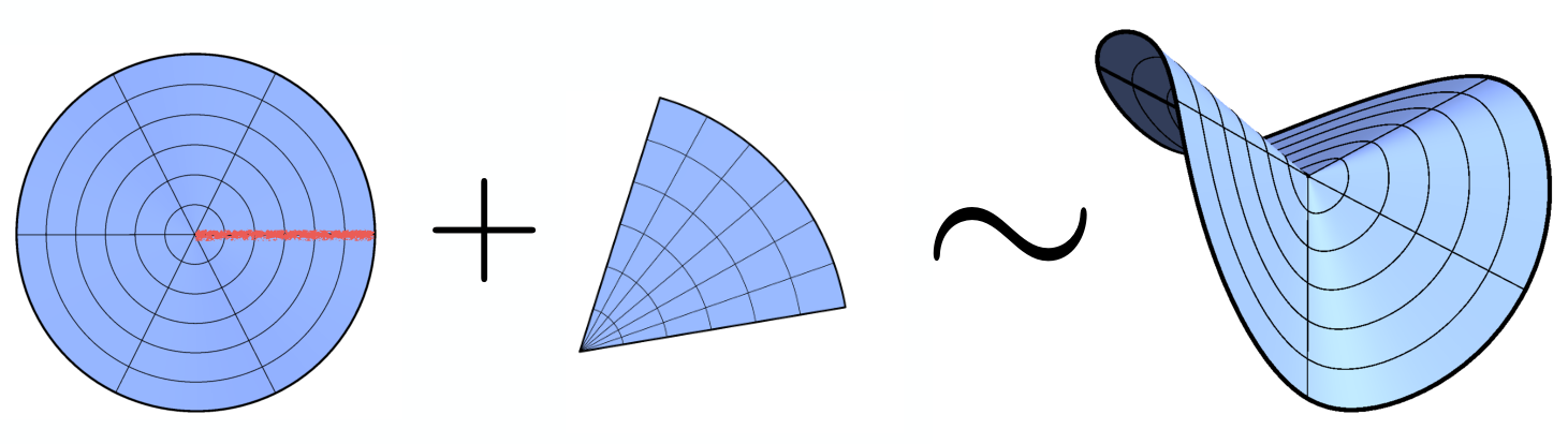
Therefore we expect that saddles to look like surplus angles (depicted in fig. 4) on intermediate slices of AdS₃ .

Going beyond the leading behavior of each saddle at small $z$ is straightforward and can be determined directly from the small $z$ expansion of (1.4). This is because all dependence on the index $p$ for the saddle enters in the combination $(\alpha_{I}+2p)^{2}$, so the corresponding subleading saddle is the same as the leading saddle for a conformal block with $h_{I}=c\Big(1-(\alpha_{I}+2p)^{2}\Big)/24$. The first few correction terms to (2.13) can easily be determined this way, e.g.

$\displaystyle\kappa\approx 12\eta_{L}(1-z)+\frac{2-z}{8}\left((\alpha_{I}+2p)^{2}-1\right)+{\cal O}(z^{2}).$

(2.19)

In all examples where we can compute $\kappa(z)$, it has a finite radius of convergence around $z\sim 0$. However, branch cuts develop at larger $z$, and we now turn to methods that will allow us to determine its behavior far from the OPE sheet.

We want to study the configuration of CFT operators depicted in figure 5, which can be interpreted as the 2-pt function of ${\cal O}_{L}$ in the background of an energy (dilatation) eigenstate:

$\displaystyle\langle{\cal O}_{H}(\infty)|{\cal O}_{L}(t_{1}){\cal O}_{L}(t_{2})|{\cal O}_{H}(-\infty)\rangle.$

(2.20)

Here the CFT lives on a cylinder, and $t=t_{1}-t_{2}$ is a Lorentzian time separation. The ${\cal O}_{H}$ operators act in the infinite past and future and create a primary state, and so the correlator will be independent of the average time $t_{1}+t_{2}$. Thus $t$ and a relative angular coordinate on the cylinder will be the only physical variables.

This Lorentzian correlator can be obtained from the usual Euclidean 4-pt function,

$\displaystyle\langle{\cal O}_{H}(\infty){\cal O}_{H}(1){\cal O}_{L}(z,\bar{z}){\cal O}_{L}(0)\rangle,$

(2.21)

by the substitution $z\to 1-e^{-it+i\phi}$ and $\bar{z}\to 1-e^{-it-i\phi}$ and a simple overall rescaling, which is necessary to pass from the plane to the cylinder. Perhaps it is surprising that ${\cal O}_{H}(\infty)$ and ${\cal O}_{H}(0)$ in the Euclidean plane immediately produce the desired eigenstates in the infinite Lorentzian future and past. This follows from the standard $i\epsilon$ prescription: to pick out the lowest-energy state created by ${\cal O}_{H}$, we must give time a small imaginary part as we push the operator insertion into the infinite future or past, and we are left with $\lim_{T\to\pm\infty}{\cal O}_{H}(e^{\epsilon T})$ which becomes ${\cal O}_{H}(0)$ or ${\cal O}_{H}(\infty)$. The analytic continuations of ${\cal O}_{L}(0)$ and ${\cal O}_{L}(z)$ are conventional; for a nice review in this context see [54].

Thus as $t\to t+2\pi$, the $z$ coordinate encircles $1$. Because both correlators and conformal blocks typically have branch cuts from $1$ to $\infty$, we will pass onto a new sheet in the complex $z$-plane, as depicted in figure 5. The late time behavior will therefore be governed by the change in the value of the correlator or Virasoro block between sheets.

In section 2.1, we saw that it is useful to compute the semiclassical Virasoro blocks ${\cal V}=e^{-\frac{c}{6}f(z)}$ by writing $f$ in terms of a function $\kappa$:

$\displaystyle f(z)=\int^{z}\frac{dx}{(1-x)x}\kappa(x).$

(2.22)

At late times, $z$ will encircle $1$ again and again, so that the leading late-time behavior will be given by the residue $2\pi i\kappa(1)$. This dramatically simplifies our task to the computation of a single number!⁷⁷ 7 Strictly speaking, we will see that $\kappa(z)$ for $z\sim 1$ has non-trivial dependence on the phase of $1-z$, so it is a bit of an abuse of notation at this point to write $\kappa(1)$. However, we will see that in the limit $t\rightarrow\pm\infty$, $\kappa(1-\epsilon e^{-it})$ approaches a constant, which is all that is needed in the present discussion. Astute readers might also worry about encountering forbidden singularities, but these are only present on the Euclidean sheet, and do not interfere with the large time analysis.

As an example of how this works, let us re-interpret the results of [1] in this light; we will also note two potential pitfalls. In [1] we found the leading saddle has

$\displaystyle\kappa(z)\approx 6z\frac{\eta_{L}\left(\alpha_{H}-1+(1-z)^{\alpha_{H}}(1+\alpha_{H})\right)-\eta_{I}\alpha_{H}(1-z)^{\frac{\alpha_{H}}{2}}}{1-(1-z)^{\alpha_{H}}}$

(2.23)

to leading order in $\eta_{L}$ and $\eta_{I}$, where $\alpha_{H}\equiv\sqrt{1-24\eta_{H}}$. When $\alpha_{H}$ is positive and real, we can take the limit $z\to 1$ unambiguously to find

$\displaystyle\kappa(1)\approx 6\eta_{L}(\alpha_{H}-1).$

(2.24)

The dependence on $\eta_{I}$ has dropped out entirely. Continuing to $\eta_{H}>\frac{c}{24}$, we find the late-time decay of the semiclassical Virasoro block

$\displaystyle{\cal V}\sim e^{-2\pi T_{H}h_{L}t},$

(2.25)

in agreement with previous results. However, this analysis neglected two important questions: how can we control potentially non-analytic behavior of $\kappa(z)$ near $z=1$, and how do we know that the semiclassical blocks are exponentially decaying, rather than exponentially growing?

We will deal with the first question by explicitly computing the leading non-analytic pieces of $\kappa(z)$ as a function of $z-1$. In our example here, it is easy to see that when $z=1-e^{-it}$ and $\alpha_{H}$ is imaginary, at late times the non-analytic pieces such as $(1-z)^{\alpha_{H}}$ vanish at late times.⁸⁸ 8 Or for the opposite choice of sign of $\alpha_{H}$, these terms grow in such a way that there is a cancellation between numerator and denominator in equation (2.23), so we obtain identical late-time behavior. We will obtain similar results for the general semiclassical blocks. The resolution to the second issue relates closely to that of the first. Just as the perturbative (in $\frac{h_{L}}{c}$) solution for $\kappa$ flipped sign at $t\to-\infty$ as compared to $t\to+\infty$, the general solutions will also be dominated by different terms in these two regimes, so that we find decay rather than growth whenever $|t|\to\infty$. We also demonstrate the transition between these two behaviors numerically in section 3.

In this section we will compute $\kappa(z)\equiv z(1-z)\partial_{z}f(z)$, where ${\cal V}=e^{-\frac{c}{6}f(z)}$, to leading order in an expansion in small $|1-z|$. As we have discussed in section 2.2, this is sufficient to determine the late time behavior of the Virasoro conformal blocks in the semiclassical limit of $c\to\infty$ with all $h_{i}/c$ fixed. Note in particular that the phase of $1-z$ can be large, as it is only the absolute value of this quantity which is presumed small.

Our strategy will be to divide the monodromy path pictured in figure 7 into two regions where (A) $y$ is far from $z$ and $1$ and (B) where $y$ and $z$ both approach $1$.⁹⁹ 9 More precisely, region A is defined as the limit $z\rightarrow 1$ with $y$ fixed, and region B as the limit $z\rightarrow 1$ with the ratio $\frac{1-y}{1-z}$ fixed. Remarkably, it is possible to solve equation (2.2) exactly in both limits. Then we will compute the full monodromy matrix $M$ as the product of four matrices: the monodromy from circling $0$ using solutions in region (A), a matching matrix between the two regions, the monodromy from region (B) and encircling $z$, and a final matching matrix.

We begin by studying equation (2.2) in region A, and so we take the limit $z\to 1$ immediately. From figure 7, this should be a good approximation when $y$ is far from both $z$ and $1$, but it must break down as $y$ passes between these two points because $T(y;z)$ has singularities when $y=z$ or $1$. Equation (2.2) at $z=1$ simply becomes a hypergeometric differential equation after a re-definition of parameters¹⁰¹⁰ 10 Here and throughout this section, $C$ is a hypergeometric parameter unrelated to the central charge.

	$\displaystyle\eta_{H}$	$\displaystyle=$	$\displaystyle\frac{1}{24}\left(1-(A-B)^{2}\right),$
	$\displaystyle\eta_{L}$	$\displaystyle=$	$\displaystyle\frac{1}{24}(2-C)C,$
	$\displaystyle\kappa$	$\displaystyle=$	$\displaystyle\frac{1}{2}C(A+B-1)-AB.$		(2.26)

We will write the solutions as

	$\displaystyle\psi_{11}$	$\displaystyle=$	$\displaystyle y^{C/2}(1-y)^{\frac{1}{2}(A+B-C+1)}\,_{2}F_{1}(A,B;C;y),$		(2.27)
	$\displaystyle\psi_{21}$	$\displaystyle=$	$\displaystyle y^{1-\frac{C}{2}}(1-y)^{\frac{1}{2}(A+B-C+1)}\,_{2}F_{1}(A-C+1,B-C+1;2-C;y).$		(2.28)

These solutions have the simple monodromy matrix

$\displaystyle\left(\begin{array}[]{cc}e^{i\pi C}&0\\ 0&e^{-i\pi C}\end{array}\right)$

as $y$ encircles $0$, which is labeled as region A in figure 3.

To solve in region B, we will change coordinates to

$\displaystyle Z\equiv 1-z,\qquad W\equiv\frac{y-z}{1-z},$

(2.32)

so that region B is the limit $|Z|\ll 1$ with $W$ fixed, and the path B shown in fig 7 is just $W\rightarrow e^{2\pi i}W$. Expanding equation (2.2) to leading order at small $Z$ leads to another hypergeometric differential equation, with solutions

	$\displaystyle\psi_{12}$	$\displaystyle=$	$\displaystyle W^{C/2}(1-W)^{\frac{1}{2}(A-B+1)}\,_{2}F_{1}(A,C-B;C;W),$		(2.33)
	$\displaystyle\psi_{22}$	$\displaystyle=$	$\displaystyle W^{1-\frac{C}{2}}(1-W)^{\frac{1}{2}(A-B+1)}\,_{2}F_{1}(1-B,A-C+1;2-C;W),$		(2.34)

which are completely independent of $Z$. Once again, it is very easy to determine these solutions’ relevant monodromy because we need only expand at small $W$, where the solutions behave as simple power-laws. In fact, as a $2\times 2$ matrix the monodromy from encircling $z$ in region B is identical to that from circling $0$ in region A.

The only remaining challenge is to match the solutions between region $A$ and $B$ in the regime where they are both valid, namely $|W|\gg 1$ and $|1-y|\ll 1$. This can be accomplished with some standard hypergeometric identities,¹¹¹¹ 11 For reference, it is useful to note that $\,{}_{2}F_{1}(A,B;C;y)$ $\displaystyle=$ $\displaystyle\frac{\Gamma(C)(1-y)^{-A-B+C}\Gamma(A+B-C)\,_{2}F_{1}(C-A,C-B;-A-B+C+1;1-y)}{\Gamma(A)\Gamma(B)}$ (2.35) $\displaystyle+\frac{\Gamma(C)\Gamma(-A-B+C)\,_{2}F_{1}(A,B;A+B-C+1;1-y)}{\Gamma(C-A)\Gamma(C-B)}$ in order to transform from solutions near $y=0$ to those near $y=1$ and vice versa. Also $\,{}_{2}F_{1}(A,B;C;y)=(1-y)^{-A-B+C}\,_{2}F_{1}(C-A,C-B;C;y)$ (2.36) can be useful when matching. and can be summarized by a $2\times 2$ matrix $M_{match}$ defined by

$\displaystyle\left(\begin{array}[]{c}\psi_{11}\\ \psi_{12}\end{array}\right)$

$\displaystyle=$

$\displaystyle M_{match}\left(\begin{array}[]{c}\psi_{21}\\ \psi_{22}\end{array}\right),$

in the regime of overlapping validity of the two solutions. The result $M_{match}$ is fairly complicated algebraically, but the end result is given in terms of it by the product.

$\displaystyle M=\left(\begin{array}[]{cc}e^{i\pi C}&0\\ 0&e^{-i\pi C}\end{array}\right)\cdot M_{match}\cdot\left(\begin{array}[]{cc}e^{i\pi C}&0\\ 0&e^{-i\pi C}\end{array}\right)\cdot M_{match}^{-1}$

Note that $\det M=1$ automatically, and so the eigenvalues of $M$ will be entirely determined by its trace. To leading order at small $Z$, the trace can be written

$\displaystyle\boxed{{\rm Tr}(M)=2-2m_{+}m_{-}-m_{+}^{2}Z^{A+B-C}-m_{-}^{2}Z^{C-A-B}}\ ,$

(2.47)

where it is convenient to separate out the coefficients of the different powers of $Z$ that appear at this order:

	$\displaystyle m_{+}$	$\displaystyle=$	$\displaystyle\frac{2\pi\Gamma(C-A-B)\Gamma(C-A-B+1)}{\Gamma(1-A)\Gamma(1-B)\Gamma(C-A)\Gamma(C-B)},$
	$\displaystyle m_{-}$	$\displaystyle=$	$\displaystyle\frac{2\pi\Gamma(A+B-C)\Gamma(A+B-C+1)}{\Gamma(A)\Gamma(B)\Gamma(A-C+1)\Gamma(B-C+1)}.$		(2.48)

The product $m_{+}m_{-}$ that appears in the $Z$-independent term can be written purely in terms of sines:

$\displaystyle m_{+}m_{-}=\frac{4\sin(\pi A)\sin(\pi B)\sin(\pi(A-C))\sin(\pi(B-C))}{\sin^{2}(\pi(A+B-C))}.$

(2.49)

Equation (2.47) is a key result in this paper, and it contains the information that we will need to determine the late time behavior of all Virasoro conformal blocks. We expect that deviations from equation (2.47) at higher order in $Z$ will take the form of a power series in $Z$ multiplying each of the terms of order $Z^{0},Z^{A+B-C}$, and $Z^{C-A-B}$. This means that the non-analyticity of the monodromy near $Z=0$ is fully captured by equation (2.47).¹²¹² 12 The series coefficients of the higher order terms in $Z$ can have singularities at some values of $A,B,C$, and for such values the higher order terms would not be negligible. The fact that the non-analyticity is captured by eq. (2.47) means that the size of such correction terms can be diagnosed on the first sheet of the complex $z$ plane, where a numeric analysis of the monodromy differential equation is straightforward.

To analyze the solutions for $\kappa(z)$ near $Z=0$, we must first discuss the relative size of the terms in the trace (2.47). As depicted in fig. 6, the limit $|Z|\rightarrow 0$ should not be thought of simply as $Z=0$, since for any small finite value $Z=1-z$ has a phase that depends on Lorentzian time. Furthermore, as time evolves $Z$ repeatedly crosses branch cuts, which typically extend from $1$ to $\infty$. These observation are crucial for understanding the relative size of the terms equation (2.47), since even for fixed $|Z|$ their relative size will be time-dependent.

We can parameterize the real and imaginary parts of $Z$ as in fig. 6,

$\displaystyle Z$

$\displaystyle=$

$\displaystyle\epsilon e^{-it},$

(2.50)

where $\epsilon$ and $t$ are real. The approximations leading to the formula (2.47) for the trace assumed $\epsilon\ll 1$, but $t$ can take any value. So the magnitude

$\displaystyle|Z^{A+B-C}|=e^{t\textrm{Im}(A+B-C)-\textrm{Re}(A+B-C)\log(1/\epsilon)}$

(2.51)

depends on time $t$ and generically transitions from small values to large values around $t\sim\frac{\textrm{Re}(A+B-C)\log\epsilon^{-1}}{\textrm{Im}(A+B-C)}$ unless the imaginary part of $A+B-C$ vanishes. Of course, this quantity depends on $\kappa$ itself via

$\displaystyle A+B-C$

$\displaystyle=$

$\displaystyle\pm\sqrt{\alpha_{H}^{2}+\alpha_{L}^{2}-4\kappa-1},$

(2.52)

so it is not quite correct to treat $A+B-C$ as a constant for all $t$. We will see, however, that all solutions have the property that $A,B,C$ approach fixed values at large $t$.

We will find two classes of solutions: those with $A+B-C\neq 0$ at large times, and those where $A+B-C\to 0$. For the former, from (2.51) we expect that either $|Z^{A+B-C}|$ or its inverse will diverge at late times. So our strategy will be to find all solutions for $\kappa$ assuming that one of $|Z^{\pm(A+B-C)}|$ is large, and then to check for self-consistency of this assumption once we have the solutions in hand. Then we will study the case $A+B-C\to 0$, finding a separate class of solutions to the monodromy condition.

Note that at generic intermediate times the monodromy condition ${\rm Tr}(M)=-2\cos\pi\alpha_{I}$ is quite complicated; we will solve it numerically in section 3, demonstrating the validity of our analytic solutions, and showing how they interpolate between small and large times.

References

- [1] A. L. Fitzpatrick, J. Kaplan, and M. T. Walters, “Universality of Long-Distance AdS Physics from the CFT Bootstrap,” JHEP 1408 (2014) 145, arXiv:1403.6829 [hep-th].
- [2] A. L. Fitzpatrick, J. Kaplan, and M. T. Walters, “Virasoro Conformal Blocks and Thermality from Classical Background Fields,” arXiv:1501.05315 [hep-th].
- [3] A. L. Fitzpatrick, J. Kaplan, M. T. Walters, and J. Wang, “Hawking from Catalan,” arXiv:1510.00014 [hep-th].
- [4] K. B. Alkalaev and V. A. Belavin, “Classical conformal blocks via AdS/CFT correspondence,” JHEP 08 (2015) 049, arXiv:1504.05943 [hep-th].
- [5] K. B. Alkalaev and V. A. Belavin, “Monodromic vs geodesic computation of Virasoro classical conformal blocks,” arXiv:1510.06685 [hep-th].
- [6] E. Hijano, P. Kraus, and R. Snively, “Worldline approach to semi-classical conformal blocks,” arXiv:1501.02260 [hep-th].
- [7] M. Beccaria, A. Fachechi, and G. Macorini, “Virasoro vacuum block at next-to-leading order in the heavy-light limit,” arXiv:1511.05452 [hep-th].
- [8] T. Anous, T. Hartman, A. Rovai, and J. Sonner, “Black Hole Collapse in the 1/c Expansion,” arXiv:1603.04856 [hep-th].
- [9] M. Besken, A. Hegde, E. Hijano, and P. Kraus, “Holographic conformal blocks from interacting Wilson lines,” arXiv:1603.07317 [hep-th].
- [10] A. L. Fitzpatrick and J. Kaplan, “Conformal Blocks Beyond the Semi-Classical Limit,” arXiv:1512.03052 [hep-th].
- [11] A. L. Fitzpatrick, J. Kaplan, D. Li, and J. Wang, “On Information Loss in AdS3/CFT2,” arXiv:1603.08925 [hep-th].
- [12] H. Chen, A. L. Fitzpatrick, J. Kaplan, D. Li, and J. Wang, “Degenerate Operators and the Expansion: Lorentzian Resummations, High Order Computations, and Super-Virasoro Blocks,” arXiv:1606.02659 [hep-th].
- [13] J. M. Maldacena, “Eternal black holes in anti-de Sitter,” JHEP 04 (2003) 021, arXiv:hep-th/0106112 [hep-th].
- [14] J. L. F. Barbon and E. Rabinovici, “Geometry And Quantum Noise,” Fortsch. Phys. 62 (2014) 626–646, arXiv:1404.7085 [hep-th].
- [15] J. Maldacena, D. Simmons-Duffin, and A. Zhiboedov, “Looking for a bulk point,” arXiv:1509.03612 [hep-th].
- [16] T. Hartman, “Entanglement Entropy at Large Central Charge,” arXiv:1303.6955 [hep-th].
- [17] C. T. Asplund, A. Bernamonti, F. Galli, and T. Hartman, “Holographic Entanglement Entropy from 2d CFT: Heavy States and Local Quenches,” arXiv:1410.1392 [hep-th].
- [18] P. Caputa, J. Simon, A. Stikonas, and T. Takayanagi, “Quantum Entanglement of Localized Excited States at Finite Temperature,” arXiv:1410.2287 [hep-th].
- [19] A. Lewkowycz, G. J. Turiaci, and H. Verlinde, “A CFT Perspective on Gravitational Dressing and Bulk Locality,” arXiv:1608.08977 [hep-th].
- [20] B. Chen, J.-q. Wu, and J.-j. Zhang, “Holographic Description of 2D Conformal Block in Semi-classical Limit,” arXiv:1609.00801 [hep-th].
- [21] A. Belavin, A. M. Polyakov, and A. Zamolodchikov, “Infinite Conformal Symmetry in Two-Dimensional Quantum Field Theory,” Nucl.Phys. B241 (1984) 333–380.
- [22] A. Zamolodchikov, “Conformal Symmetry in Two-dimensional Space: Recursion Representation of the Conformal Block,” Teoreticheskaya i Matematicheskaya Fizika 73 (1987) 103–110.
- [23] E. Witten, “Quantum Field Theory and the Jones Polynomial,” Commun. Math. Phys. 121 (1989) 351–399.
- [24] E. Witten, “(2+1)-Dimensional Gravity as an Exactly Soluble System,” Nucl. Phys. B311 (1988) 46.
- [25] H. L. Verlinde, “Conformal Field Theory, 2- Quantum Gravity and Quantization of Teichmuller Space,” Nucl. Phys. B337 (1990) 652.
- [26] S. Elitzur, G. W. Moore, A. Schwimmer, and N. Seiberg, “Remarks on the Canonical Quantization of the Chern-Simons-Witten Theory,” Nucl. Phys. B326 (1989) 108.
- [27] E. Witten, “Analytic Continuation Of Chern-Simons Theory,” AMS/IP Stud. Adv. Math. 50 (2011) 347–446, arXiv:1001.2933 [hep-th].
- [28] D. Gaiotto and E. Witten, “Knot Invariants from Four-Dimensional Gauge Theory,” Adv. Theor. Math. Phys. 16 no. 3, (2012) 935–1086, arXiv:1106.4789 [hep-th].
- [29] D. Dorigoni, “An Introduction to Resurgence, Trans-Series and Alien Calculus,” arXiv:1411.3585 [hep-th].
- [30] G. V. Dunne and M. Unsal, “Resurgence and Trans-series in Quantum Field Theory: The CP(N-1) Model,” JHEP 11 (2012) 170, arXiv:1210.2423 [hep-th].
- [31] G. Basar, G. V. Dunne, and M. Unsal, “Resurgence theory, ghost-instantons, and analytic continuation of path integrals,” JHEP 10 (2013) 041, arXiv:1308.1108 [hep-th].
- [32] A. Cherman, D. Dorigoni, and M. Unsal, “Decoding perturbation theory using resurgence: Stokes phenomena, new saddle points and Lefschetz thimbles,” JHEP 10 (2015) 056, arXiv:1403.1277 [hep-th].
- [33] G. V. Dunne, M. Shifman, and M. Unsal, “IR Renormalons vs. Operator Product Expansion in Supersymmetric and Related Gauge Theories,” arXiv:1502.06680 [hep-th].
- [34] G. V. Dunne and M. Unsal, “Deconstructing zero: resurgence, supersymmetry and complex saddles,” arXiv:1609.05770 [hep-th].
- [35] C. Kozcaz, T. Sulejmanpasic, Y. Tanizaki, and M. Unsal, “Cheshire Cat resurgence, Self-resurgence and Quasi-Exact Solvable Systems,” arXiv:1609.06198 [hep-th].
- [36] I. Aniceto, R. Schiappa, and M. Vonk, “The Resurgence of Instantons in String Theory,” Commun. Num. Theor. Phys. 6 (2012) 339–496, arXiv:1106.5922 [hep-th].
- [37] R. Schiappa and R. Vaz, “The Resurgence of Instantons: Multi-Cut Stokes Phases and the Painleve II Equation,” Commun. Math. Phys. 330 (2014) 655–721, arXiv:1302.5138 [hep-th].
- [38] I. Aniceto and R. Schiappa, “Nonperturbative Ambiguities and the Reality of Resurgent Transseries,” Commun. Math. Phys. 335 no. 1, (2015) 183–245, arXiv:1308.1115 [hep-th].
- [39] R. Couso-Santamaría, R. Schiappa, and R. Vaz, “Finite N from Resurgent Large N,” Annals Phys. 356 (2015) 1–28, arXiv:1501.01007 [hep-th].
- [40] G. ’t Hooft, “Can We Make Sense Out of Quantum Chromodynamics?,” Subnucl. Ser. 15 (1979) 943.
- [41] P. C. Argyres and M. Unsal, “The semi-classical expansion and resurgence in gauge theories: new perturbative, instanton, bion, and renormalon effects,” JHEP 08 (2012) 063, arXiv:1206.1890 [hep-th].
- [42] G. V. Dunne and M. Unsal, “Uniform WKB, Multi-instantons, and Resurgent Trans-Series,” Phys. Rev. D89 no. 10, (2014) 105009, arXiv:1401.5202 [hep-th].
- [43] V. S. Dotsenko and V. A. Fateev, “Conformal Algebra and Multipoint Correlation Functions in Two-Dimensional Statistical Models,” Nucl. Phys. B240 (1984) 312.
- [44] V. S. Dotsenko and V. A. Fateev, “Four Point Correlation Functions and the Operator Algebra in the Two-Dimensional Conformal Invariant Theories with the Central Charge c ¡ 1,” Nucl. Phys. B251 (1985) 691.
- [45] P. Di Francesco, P. Mathieu, and D. Senechal, Conformal Field Theory. Graduate Texts in Contemporary Physics. Springer-Verlag, New York, 1997. http://www-spires.fnal.gov/spires/find/books/www?cl=QC174.52.C66D5::1997.
- [46] J. Maldacena, D. Stanford, and Z. Yang, “Conformal symmetry and its breaking in two dimensional Nearly Anti-de-Sitter space,” arXiv:1606.01857 [hep-th].
- [47] D. Harlow, J. Maltz, and E. Witten, “Analytic Continuation of Liouville Theory,” JHEP 1112 (2011) 071, arXiv:1108.4417 [hep-th].
- [48] E. Hijano, P. Kraus, and R. Snively, “Worldline approach to semi-classical conformal blocks,” JHEP 07 (2015) 131, arXiv:1501.02260 [hep-th].
- [49] J. de Boer, A. Castro, E. Hijano, J. I. Jottar, and P. Kraus, “Higher spin entanglement and conformal blocks,” JHEP 07 (2015) 168, arXiv:1412.7520 [hep-th].
- [50] A. Ronveaux and F. M. Arscott, Heun’s differential equations. Clarendon Press, 1995.
- [51] A. Litvinov, S. Lukyanov, N. Nekrasov, and A. Zamolodchikov, “Classical Conformal Blocks and Painleve VI,” arXiv:1309.4700 [hep-th].
- [52] D. A. Roberts and D. Stanford, “Two-dimensional conformal field theory and the butterfly effect,” arXiv:1412.5123 [hep-th].
- [53] A. L. Fitzpatrick and J. Kaplan, “A Quantum Correction To Chaos,” arXiv:1601.06164 [hep-th].
- [54] T. Hartman, S. Jain, and S. Kundu, “Causality Constraints in Conformal Field Theory,” arXiv:1509.00014 [hep-th].
- [55] S. Deser and R. Jackiw, “Three-Dimensional Cosmological Gravity: Dynamics of Constant Curvature,” Annals Phys. 153 (1984) 405–416.
- [56] G. Turiaci and H. Verlinde, “On CFT and Quantum Chaos,” arXiv:1603.03020 [hep-th].
- [57] M. Bauer, P. Di Francesco, C. Itzykson, and J. B. Zuber, “Singular vectors of the Virasoro algebra,” Phys. Lett. B260 (1991) 323–326.
- [58] M. Bauer, P. Di Francesco, C. Itzykson, and J. B. Zuber, “Covariant differential equations and singular vectors in Virasoro representations,” Nucl. Phys. B362 (1991) 515–562.
- [59] M. Headrick, “Entanglement Renyi entropies in holographic theories,” Phys.Rev. D82 (2010) 126010, arXiv:1006.0047 [hep-th].
- [60] S. Hellerman, “A Universal Inequality for CFT and Quantum Gravity,” JHEP 1108 (2011) 130, arXiv:0902.2790 [hep-th].
- [61] E. Perlmutter, “Bounding the Space of Holographic CFTs with Chaos,” arXiv:1602.08272 [hep-th].
- [62] S. Jackson, L. McGough, and H. Verlinde, “Conformal Bootstrap, Universality and Gravitational Scattering,” arXiv:1412.5205 [hep-th].
- [63] B. Chen and J.-J. Zhang, “On short interval expansion of Renyi entropy,” JHEP 1311 (2013) 164, arXiv:1309.5453 [hep-th].
- [64] C. A. Keller and A. Maloney, “Poincare Series, 3D Gravity and CFT Spectroscopy,” arXiv:1407.6008 [hep-th].
- [65] C.-M. Chang and Y.-H. Lin, “Bootstrapping 2D CFTs in the Semiclassical Limit,” arXiv:1510.02464 [hep-th].
- [66] C.-M. Chang and Y.-H. Lin, “Semiclassical OPE coefficients from 3D gravity,” arXiv:1604.01774 [hep-th].
- [67] N. Benjamin, E. Dyer, A. L. Fitzpatrick, and S. Kachru, “Universal Bounds on Charged States in 2d CFT and 3d Gravity,” arXiv:1603.09745 [hep-th].
- [68] P. Caputa, J. Simon, A. Stikonas, T. Takayanagi, and K. Watanabe, “Scrambling time from local perturbations of the eternal BTZ black hole,” JHEP 08 (2015) 011, arXiv:1503.08161 [hep-th].
- [69] A. Galliani, S. Giusto, E. Moscato, and R. Russo, “Correlators at large c without information loss,” arXiv:1606.01119 [hep-th].
- [70] P. Kraus and A. Maloney, “A Cardy Formula for Three-Point Coefficients: How the Black Hole Got its Spots,” arXiv:1608.03284 [hep-th].
- [71] D. Friedan and C. A. Keller, “Constraints on 2d CFT partition functions,” JHEP 10 (2013) 180, arXiv:1307.6562 [hep-th].
- [72] T. Hartman, C. A. Keller, and B. Stoica, “Universal Spectrum of 2d Conformal Field Theory in the Large c Limit,” JHEP 1409 (2014) 118, arXiv:1405.5137 [hep-th].
- [73] I. Esterlis, A. L. Fitzpatrick, and D. Ramirez, “Closure of the Operator Product Expansion in the Non-Unitary Bootstrap,” arXiv:1606.07458 [hep-th].
- [74] B. Ponsot and J. Teschner, “Liouville bootstrap via harmonic analysis on a noncompact quantum group,” arXiv:hep-th/9911110 [hep-th].
- [75] J. Teschner, “A Lecture on the Liouville vertex operators,” Int. J. Mod. Phys. A19S2 (2004) 436–458, arXiv:hep-th/0303150 [hep-th].
- [76] P. Caputa, T. Numasawa, and A. Veliz-Osorio, “Scrambling without chaos in RCFT,” arXiv:1602.06542 [hep-th].
- [77] A. L. Fitzpatrick, J. Kaplan, D. Poland, and D. Simmons-Duffin, “The Analytic Bootstrap and AdS Superhorizon Locality,” JHEP 1312 (2013) 004, arXiv:1212.3616 [hep-th].
- [78] Z. Komargodski and A. Zhiboedov, “Convexity and Liberation at Large Spin,” JHEP 1311 (2013) 140, arXiv:1212.4103 [hep-th].