Inferring dissipation from current fluctuations

Experiments capable of probing molecular-scale dynamics have led to a wealth of data about the operation of nanoscale machines [1, 2, 3]. Like their macroscopic counterparts, nanomachines convert free energy from the environment into useful work. Due to molecular fluctuations, however, nanoscale machines behave stochastically. Though the stochasticity renders nanomachines less predictable, the fluctuations also offers a unique tool to deduce additional physical properties of the machine. Indeed, the fluctuation-dissipation theorem (FDT) demonstrates that near-equilibrium fluctuations allow one to deduce the nonequilibrium response to small perturbations, an idea that has become a central theme of statistical mechanics [4, 5, 6, 7, 8, 9]. Analogous exploitation of far-from-equilibrium fluctuations is highly desirable [10, 11, 12, 13, 14], particularly for studying living systems [15, 16, 17].

In this work, we demonstrate how it is possible to extract information from nonequilibrium fluctuations under general steady-state conditions. Our central assumption is that the mesoscale dynamics, in a quantum or a classical system, can be described by a Markovian stochastic process. For example, the Markovian mesoscopic description applies to biochemical kinetics of enzymatic reactions. In this context, dynamical fluctuations have been used to constrain proposed models for enzymatic pathways, providing bounds on the number of distinct intermediate states [18, 19]. More recently, advances in the theory of Markov processes [20, 21, 22, 23] have been used to relate the dynamical fluctuations to the physical dissipation rate of the nonequilibrium dynamics [24, 25, 26, 27]. This paper reviews and extends that connection between fluctuations and dissipation, a connection which can be thought of as a generalization of the FDT. Where the FDT offers an equality—by measuring fluctuations we may determine the dissipation exactly [28]—the far-from-equilibrium analog guarantees an inequality: the extent of fluctuations sets a lower bound on the dissipation rate. Hence experimental observations of macroscopic, coarse-grained fluctuations provide enough information to estimate a bound on the dissipation rate of a process far from equilibrium.

In this paper, we study this generalization of the FDT bound from the perspective of coarse-graining, a viewpoint which we anticipate will complement experimental applications. After reviewing the formalism of Markov jump processes in Section II, we consider the consequence of temporal coarse-graining in Section III. By focusing on dynamical quantities which are time-averaged over long trajectories, we arrive at the so-called Level 2.5 large deviations, which quantify dynamical fluctuations in the jump process [20, 21, 22, 23]. Mirroring our previous work [26], Section IV develops our central relationship between nonequilibrium dynamical fluctuations and dissipation. In its most general form, the relationship pertains to a fluctuating vector quantity in the space of all microscopic currents; the implication for scalar currents is detailed in Section V. In addition to the temporal coarse-graining, we investigate the role of spatial resolution by studying two limits: a diffusive limit in Section VI and the spatial coarse-graining of a particular diffusion process in Section VII. A consequence of the coarse-graining is that the macrostate dynamics may not be Markovian. Remarkably, even without the Markov property, coarse-grained fluctuations can bound the dissipation rate so long as the macroscopic dynamics emerges from an underlying Markovian description, suggesting that suitable analysis of dynamical fluctuations can complement existing methods for deducing dissipation from time series data [29].

The Markov jump process has rich temporal correlations—after a short time, a system initialized in mesostate $y$ is more likely to be in a neighboring state $z$ than the steady-state probability $\pi(z)$ would predict. Though these correlations add complexity to transient dynamics, they die out after some finite correlation time. The empirical density and empirical current can be averaged over sufficiently long times $T$ such that the transient dynamics becomes unimportant. In this way, $\boldsymbol{p}$ and $\boldsymbol{j}$ can be thought of as the result of temporal coarse-graining with a coarse-graining timescale exceeding natural correlation times. In the limit of large $T$, the empirical fluctuations can therefore be mimicked by Poisson point processes, which lack all temporal correlations. More specifically, the coarse-grained Markov jump process resembles the behavior of a collection of independent Poisson point processes, one per directed edge of the graph, which count the number of transition events for each edge in time $T$. The large deviation structure of Poisson processes are particularly simple, providing a heuristic route to $I(\boldsymbol{p},\boldsymbol{j})$ for a general nonequilibrium jump process. Rigorous derivations of this result utilize a technique called Cramér tilting [21]. Rather than recapitulate that argument, we illustrate how the form of the jump process rate function originates from a Poisson point process.

To relate the fluctuations described by the rate function $I(\boldsymbol{p},\boldsymbol{j})$ to the thermodynamic dissipation, it is useful to write $I$ in terms of the currents and thermodynamic forces $\boldsymbol{F}^{p}$. For notational compactness we suppress the labels of the vertices. We note that $j^{p}/\sinh(F^{p}/2)=a^{p}\geq 0$, implying that $j^{p}$ has the same sign as $F^{p}$. Furthermore, it is natural to measure the empirical current $j$ relative to the current $j^{p}$, so we introduce $\bar{\jmath}\equiv j/j^{p}$. With this new notation,

Taylor expanding in powers of $F^{p}$, we obtain

The low-order partial sums of this series alternate, first overestimating, then underestimating $\Psi$ (see Fig. 3). In particular, the first partial sum bounds the rate function by a quadratic [26],

where $\sigma^{p}=j^{p}F^{p}$ is the local dissipation for the edge.

Truncation of a Taylor series, of course, does not necessarily yield a bound. To prove inequality (27) we must confirm the positivity of the residual $\Delta\equiv\Psi_{\rm quad}-\Psi$. Since $\Delta$ is symmetric about $\bar{\jmath}=0$, it suffices to consider positive $\bar{\jmath}$. We note that $\Delta$ vanishes when $\bar{\jmath}=1$, and

implying that $\Delta$ strictly increases as $|\bar{\jmath}-1|$ grows ⁴⁴ 4 Using the monotonicity of arcsinh and the concavity of $\sinh$, Eq. (28) implies that $\partial\Delta/\partial\bar{\jmath}>0$ for $\bar{\jmath}>1$ and $\partial\Delta/\partial\bar{\jmath}<0$ for $0\leq\bar{\jmath}\leq 1$.. Since $\Psi\leq\Psi_{\rm quad}$ is bounded for every edge of the graph, $I(\boldsymbol{p},\boldsymbol{j})$ is bounded by a quadratic form whose curvature is determined by the local dissipation rates:

Eq. (29) is restricted to conservative currents, or alternatively we take $I_{\rm quad}\equiv\infty$ for nonconservative $\boldsymbol{j}$.

Recall that by construction $I(\boldsymbol{\pi},\boldsymbol{j}^{\pi})=0$. Our quadratic bound shares this minimum. Furthermore, $I(\boldsymbol{\pi},-\boldsymbol{j}^{\pi})=I_{\rm quad}(\boldsymbol{\pi},-\boldsymbol{j}^{\pi})$, so $I_{\rm quad}$ is the tightest quadratic upper bound which has a minimum at $(\boldsymbol{\pi},\boldsymbol{j}^{\pi})$ and can be expressed as a single sum over edges (i.e., is diagonal in the edge basis) [27]. The curvature of $I$, evaluated at $\boldsymbol{\pi}$ and $\boldsymbol{j}^{\pi}$, reflects the variance of long-time current fluctuations. The tighter inequality  (29) is, the more precisely we may relate this variance to the local dissipation rates. Truncation after the first-order term of the series expansion Eq. (26) becomes exact for small thermodynamic forces, meaning that the quadratic bound is accurate when $F^{p}$ is small.

The large deviation function $I(\boldsymbol{p},\boldsymbol{j})$ describes the joint distribution for the density in all mesostates and currents between these states. Experiments, however, cannot hope to resolve the statistical details of a large number of degrees of freedom. To make practical use of inequality (29), we must project the result onto a smaller probability space. Rather than monitoring $\boldsymbol{p}$ and $\boldsymbol{j}$, suppose we only measure a scalar current of the form

The generalized current $j_{d}$ is a linear combination of the currents between mesostates with expansion coefficients $\boldsymbol{d}$ [24]. This construction affords significant flexibility. By choosing $\boldsymbol{d}=\boldsymbol{F}^{\pi}$, the generalized current is the same as the dissipation rate. Other choices of $\boldsymbol{d}$ can highlight the current across a single edge or the current associated with transitions between macrostates, as illustrated in Section VII.

In the long-time limit, the distribution for this generalized current adopts the large deviation form $P(j_{d})\asymp e^{-TI(j_{d})}$. Because $P(j_{d})$ can be constructed from $P(\boldsymbol{p},\boldsymbol{j})$, the rate function for the generalized current is related to $I(\boldsymbol{p},\boldsymbol{j})$  ⁵⁵ 5 The restriction to conservative currents is built into $I$ because $I(\boldsymbol{p},\boldsymbol{j})=\infty$ for non-conservative $\boldsymbol{j}$:

This infimum is bounded from above by $I(\boldsymbol{p}^{*},\boldsymbol{j}^{*})$ for any choice of $\boldsymbol{p}^{*}$ and conservative $\boldsymbol{j}^{*}$ such that $\boldsymbol{j}^{*}\cdot\boldsymbol{d}=j_{d}$. We choose $\boldsymbol{p}^{*}=\boldsymbol{\pi}$ and $\boldsymbol{j}^{*}=(j_{d}/j_{d}^{\pi})\boldsymbol{j}^{\pi}$, where $j_{d}^{\pi}\equiv\boldsymbol{j}^{\pi}\cdot\boldsymbol{d}$. As a multiple of the conservative steady-state current $\boldsymbol{j}^{\pi}$, $\boldsymbol{j}^{*}$ is guaranteed to be conservative. Hence

where we have used inequality (29). The bound on the large deviation function translates to a bound on the variance of $j_{d}$ since $\text{var}(j_{d})=1/I^{\prime\prime}(j_{d}^{\pi})$, so measuring the mean and variance of any scalar current provides a lower bound on the dissipation rate:

The bound on $\Sigma^{\pi}$ is most useful if it is tight, but there are two distinct reasons it might be loose: (1) $\Psi$ for the edges could deviate significantly from the quadratic bound $\Psi_{\rm quad}$ or (2) our choice of $\boldsymbol{p}^{*}$ and $\boldsymbol{j}^{*}$ could be suboptimal. In the remainder of the paper we study diffusion processes as a limit of Markov jump processes. That limiting procedure yields $\Psi=\Psi_{\rm quad}$, implying that the diffusion process bound is weakened only by our suboptimal $\boldsymbol{p}^{*}$ and $\boldsymbol{j}^{*}$. For diffusions, the high-dimensional rate function $I(\boldsymbol{p},\boldsymbol{j})$ is exactly given by the quadratic $I_{\rm quad}(\boldsymbol{p},\boldsymbol{j})$, but the low-dimensional rate function $I(j_{d})$ can still differ significantly from the upper bound in inequality (32). Section VII considers this scenario in greater detail.

Though our results have been derived for Markov jump processes, we may translate them into appropriate forms to describe fluctuations in diffusion processes. For simplicity, we consider this diffusive limit only for a single particle moving in two dimensions with mobility $\mu$. Let $\boldsymbol{x}\equiv(x_{1},x_{2})$ denote the particle’s position, which evolves according to an overdamped Langevin equation with deterministic force $\boldsymbol{f}(\boldsymbol{x})\equiv(f_{1}(\boldsymbol{x}),f_{2}(\boldsymbol{x}))$ and random force $\boldsymbol{\eta}$. We further decompose the deterministic force into a contribution from a free energy gradient $\nabla U(\boldsymbol{x})$ and one from a non-gradient external field $\boldsymbol{f}_{\rm ext}(\boldsymbol{x})$,

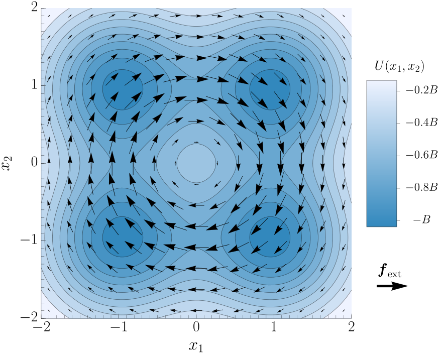
The random force at time $t$, $\boldsymbol{\eta}(t)\equiv(\eta_{1}(t),\eta_{2}(t))$ is a vector of Gaussian random variables satisfying $\left<\eta_{k}(t)\right>=0$ and $\left<\eta_{k}(t)\eta_{k^{\prime}}(t^{\prime})\right>=2D\delta_{k,k^{\prime}}\delta(t-t^{\prime})$, where $D$ is the diffusion constant. In Section VII we will consider the particular driven diffusive process shown in Fig. 4 as an illustrative example.

Associated to the Langevin equation is a Fokker-Planck equation describing the evolution of probability density at position $\boldsymbol{x}$, $\rho(\boldsymbol{x})$:

where

is the $\rho$-dependent current at $\boldsymbol{x}$. We denote the steady-state density $\rho^{\pi}$ and the steady-state current $\boldsymbol{\mathcal{J}}^{\pi}$. As in the jump process, we define an empirical density field and empirical current field, $\rho$ and $\boldsymbol{\mathcal{J}}$ respectively, and measure the probability of fluctuations away from $\rho^{\pi}$ and $\boldsymbol{\mathcal{J}}^{\pi}$ using the rate function $\mathcal{I}[\rho,\boldsymbol{\mathcal{J}}]$. The square brackets highlight that $\mathcal{I}$ is now a functional of the density and current fields. The exact form of $\mathcal{I}$ is known [38, 27]. In this section, we give a complementary derivation of the result using a limit of the Markov jump process results. The limiting procedure serves to clarify the origin of quadratic current fluctuations in diffusion processes.

To leverage our previous results, we approximate the diffusion process by a jump process on a square lattice, as depicted in Fig. 5.

There is no unique way to coarse-grain a diffusion to a jump process [39]. Thus we have freedom in how we construct our model so long as it yields a diffusive limit that matches the Fokker-Planck equation, Eq. (35), when the lattice spacing becomes infinitesimal. We construct a simple nearest-neighbor jump process which is entirely characterized by four space-dependent transition rates for hopping from a grid point at $\boldsymbol{x}$ to a nearest-neighbor site: $W_{\rm up}(\boldsymbol{x}),W_{\rm right}(\boldsymbol{x}),W_{\rm down}(\boldsymbol{x}),$ and $W_{\rm left}(\boldsymbol{x})$. These rates must scale with the lattice spacing $h$ in such a way that the first two jump moments give the correct drift and diffusion [39], requiring

as $h\to 0$. From these constraints the hopping rates are

We now identify each vertex of the graph by its location $\boldsymbol{x}$, writing the density at that vertex as $p(\boldsymbol{x})$. The edge connecting grid point $\boldsymbol{x}$ to its neighbor on the right has current $j^{p}_{\rm right}(\boldsymbol{x})\equiv j^{p}(\boldsymbol{x},\boldsymbol{x}+(h,0))$, and the thermodynamic force associated to that edge is $F^{p}_{\rm right}(\boldsymbol{x})\equiv F^{p}(\boldsymbol{x},\boldsymbol{x}+(h,0))$. The “up,” “down,” and “left” directions are treated analogously. Using this notation, we may rewrite $I_{\rm quad}$ of Eq. (29) as

To simplify the expression further, we must convert from the discrete-space density $\boldsymbol{p}$ and current $\boldsymbol{j}$ to the fields $\rho$ and $\boldsymbol{\mathcal{J}}$. In the continuum limit, $\boldsymbol{p}(\boldsymbol{x})$ vanishes while $\rho(\boldsymbol{x})$ remains finite such that $\boldsymbol{p}(\boldsymbol{x})\to h^{2}\rho(\boldsymbol{x})$. The current field $\boldsymbol{\mathcal{J}}^{\rho}$ is also finite, but the current on any edge of the lattice vanishes with order $h$:

Likewise, the thermodynamic force on each edge vanishes in proportion to $h$:

with a finite thermodynamic force field given by

Hence the ratio of force to current on an edge, which appears in each term of Eq. (39), remains finite and independent of the jump direction,

Recall from Eq. (26) that the rate function bound (29) becomes tighter for small thermodynamic forces. Since the forces vanish in the $h\to 0$ limit, the jump process on an infinitesimal grid thus saturates inequality (29), yielding the equality

In other words, approximating $I$ by $I_{\rm quad}$ becomes exact in the continuum limit. We convert the sum to an integral using

and insert Eqs. (40) and (43) into Eq. (39) to obtain the rate function for diffusions

Note that the current fluctuations are strictly quadratic, a fact that can be traced back to the vanishingly small thermodynamic force on each infinitesimal edge of the graph.

The rate function may alternatively be expressed with respect to the local dissipation rates,

Interpreting $\boldsymbol{\sigma}^{\rho}$ as a physical dissipation requires that the particle exchanges energy with a thermal reservoir at inverse temperature $\beta$ and satisfies the Einstein relation $\beta D=\mu$. The second equality follows from a rearrangement of Eq. (43),

which is an expression of linear response; the current at any point in space is linearly proportional to the thermodynamic force at that point. This linear-response feature of diffusion processes implies that the current fluctuations are specified by local dissipation rates:

Our form for $\mathcal{I}$ is analogous to the right-hand side of inequality (29), but for diffusion processes the inequality has become an equality.

Up to this point we have assumed a mesoscopic Markov process that is monitored with complete precision. More commonly, it is only possible to observe coarse-grained macrostates, and transitions between them might not be Markovian. Rather, the macroscopic dynamics is described by a hidden Markov model [40]. Remarkably, current fluctuations in the non-Markovian macroscopic dynamics carry information about the dissipation rate of the underlying mesoscopic degrees of freedom.

To illustrate the connection between dissipation and a macroscopic current, we study the generalized scalar current $j_{d}$, defined in Eq. (30). The vector $\boldsymbol{d}$ determines which microscopic transitions are observable, so for a suitable choice of $\boldsymbol{d}$, $j_{d}$ can be any macroscopic current. Consider, for example, the two-dimensional driven diffusion process in Fig. 4. A particle evolves on a free energy landscape

with $B$ controlling the depth of four Gaussian wells centered at $\boldsymbol{c}=(\pm 1,\pm 1)$. At a coarse-grained level, these wells define four possible macrostates, the quadrants of the coordinate plane. In addition to the free energy landscape, we introduce a non-gradient external field with amplitude $A$,

which drives transitions between the macrostates. By using Eq. (38) to discretize the state space, we can numericdally solve for the steady state, as plotted in Fig. 6. We focus on the macroscopic current given by the rate of clockwise (CW) transitions between these coarse-grained states less the rate of counter-clockwise (CCW) transitions. As illustrated in Fig. 7, we measure this current, $j_{d}=\boldsymbol{j}\cdot\boldsymbol{d}$, by choosing

The results from Sec. V directly apply to this construction. In particular, inequality (33) implies $\Sigma^{\pi}\geq 2(j_{d}^{\pi})^{2}/\text{var}(j_{d})$. The right-hand side of this inequality depends on the first two moments of the macroscopic empirical current distribution. By measuring these moments with coarse-grained observations, we therefore bound the total entropy production of the mesoscopic system, $\Sigma^{\pi}$.

To assess the inequality’s tightness, we used a $400\times 400$ grid to numerically compute $I(j_{d})$ for the four-well model with $D=\mu=1$, and with various choices of $A$ and $B$. We saw in Sec. VI that $I_{\rm quad}$ becomes exact in the diffusive limit, so

The numerical results, plotted in Fig. 8, reflect that inequality (53) is a tight bound for the variance. In contrast, the dissipation rate bound, inequality (32), is noticeably weaker. A measure of this weakness is the ratio

which ranges from $0$ to $1$. This ratio, plotted in Fig. 9 for a range of driving amplitudes and well depths, assesses the fraction of the dissipation rate that can be inferred from the macroscopic current fluctuations.

It has been shown that our inference strategy detects the greatest fraction of dissipation if the macroscopic current is constructed to be proportional to the thermodynamic force [26]. More precisely, $\phi=1$ when $\boldsymbol{d}\propto\boldsymbol{F}^{\pi}$, and $\phi$ decreases when the vector $\boldsymbol{d}$ is less aligned with $\boldsymbol{F}^{\pi}$. In our coarse-graining example, the elements of $\boldsymbol{d}$ are set to $0$ or $\pm 1$ based on whether each mesoscopic transition is observable. With $\boldsymbol{d}$ constrained by which transitions are observable, $\phi$ can only be varied if $\boldsymbol{F}^{\pi}$ is altered, something that can be achieved by tuning $A$ and $B$.

We can understand $\phi$’s dependence on these model parameters by analyzing the degree to which $\boldsymbol{F}^{\pi}$ aligns with $\boldsymbol{d}$. Fig. 10 illustrates how the continuous thermodynamic force field $\boldsymbol{\mathcal{F}}^{\pi}(\boldsymbol{x})$ varies with the well depth. In the absence of wells ($B=0$), the thermodynamic force is radially symmetric about the origin. As the wells are made deeper, $\boldsymbol{\mathcal{F}}^{\pi}$ is amplified along the axes, more closely resembling $\boldsymbol{d}$ of Fig. 7. This resemblance explains the trend that $\phi$ increases with increasing $B$. Interestingly, $\phi$ depends only weakly on the external field amplitude, a fact we rationalize with a linear-response argument at the end of Appendix B.

It is typically impossible to resolve detailed mesoscopic dynamics, even with the most sophisticated experimental tools. Because the dissipation rate is defined in terms of such immeasurable mesoscopic transitions, it may seem that there is no hope of experimentally measuring the dissipation, short of explicitly detecting the free energetic flows from the thermodynamic reservoirs. Our models and analysis demonstrate that, in fact, a bound on the total dissipation can be inferred by monitoring only the fluctuations in macroscopic currents. The procedure we use to infer this bound is extremely adaptable; we make essentially no assumptions about the mesoscopic details of the system nor about the macroscopic currents that will be observed.

References

- [1] S. B. Smith, L. Finzi, and C. Bustamante, Science 258, 1122 (1992).
- [2] V. Blickle and C. Bechinger, Nature Physics 8, 143 (2012).
- [3] I. A. Martínez, E. Roldán, L. Dinis, D. Petrov, J. M. R. Parrondo, and R. A. Rica, Nature Physics 12, 67 (2016).
- [4] U. M. B. Marconi, A. Puglisi, L. Rondoni, and A. Vulpiani, Physics Reports 461, 111 (2008).
- [5] A. Einstein, Annalen der Physik 322, 549 (1905).
- [6] L. Onsager, Physical Review 37, 405 (1931a).
- [7] L. Onsager, Physical Review 38, 2265 (1931b).
- [8] H. B. Callen and T. A. Welton, Physical Review 83, 34 (1951).
- [9] R. Kubo, Reports on Progress in Physics 29, 255 (1966).
- [10] T. Harada and S.-i. Sasa, Physical Review Letters 95, 130602 (2005).
- [11] T. Speck and U. Seifert, EPL (Europhysics Letters) 74, 391 (2006).
- [12] M. Baiesi, C. Maes, and B. Wynants, Physical Review Letters 103, 010602 (2009).
- [13] J. Prost, J.-F. Joanny, and J. M. R. Parrondo, Physical Review Letters 103, 090601 (2009).
- [14] U. Seifert and T. Speck, EPL (Europhysics Letters) 89, 10007 (2010).
- [15] P. Bohec, F. Gallet, C. Maes, S. Safaverdi, P. Visco, and F. Van Wijland, EPL (Europhysics Letters) 102, 50005 (2013).
- [16] É. Fodor, M. Guo, N. Gov, P. Visco, D. Weitz, and F. van Wijland, EPL (Europhysics Letters) 110, 48005 (2015).
- [17] É. Fodor, W. W. Ahmed, M. Almonacid, M. Bussonnier, N. S. Gov, M.-H. Verlhac, T. Betz, P. Visco, and F. van Wijland, EPL (Europhysics Letters) 116, 30008 (2016).
- [18] J. R. Moffitt and C. Bustamante, FEBS Journal 281, 498 (2014).
- [19] A. C. Barato and U. Seifert, The Journal of Physical Chemistry B 119, 6555 (2015a).
- [20] G. Kesidis and J. Walrand, IEEE Transactions on Information Theory 39, 1056 (1993).
- [21] C. Maes and K. Netočnỳ, EPL (Europhysics Letters) 82, 30003 (2008).
- [22] L. Bertini, A. Faggionato, and D. Gabrielli, Annales de l’Institut Henri Poincaré. Section B, Probabilités et Statistiques 51, 867 (2015a).
- [23] L. Bertini, A. Faggionato, and D. Gabrielli, Stochastic Processes and their Applications 125, 2786 (2015b).
- [24] A. C. Barato and U. Seifert, Physical Review Letters 114, 158101 (2015b).
- [25] P. Pietzonka, A. C. Barato, and U. Seifert, Physical Review E 93, 052145 (2016a).
- [26] T. R. Gingrich, J. M. Horowitz, N. Perunov, and J. L. England, Physical Review Letters 116, 120601 (2016).
- [27] M. Polettini, A. Lazarescu, and M. Esposito, Physical Review E 94, 052104 (2016).
- [28] R. Kubo, M. Toda, and N. Hashitsume, Statistical Physics II: Nonequilibrium Statistical Mechanics, Vol. 31 (Springer Science & Business Media, 2012).
- [29] É. Roldán and J. M. Parrondo, Physical Review Letters 105, 150607 (2010).
- [30] N. Van Kampen, Stochastic Processes in Physics and Chemistry, Vol. 1 (Elsevier, 1992).
- [31] K. H. Hoffmann and P. Salamon, Physica A: Statistical Mechanics and its Applications 390, 3086 (2011).
- [32] M. Esposito, Physical Review E 85, 041125 (2012).
- [33] J. D. Chodera, N. Singhal, V. S. Pande, K. A. Dill, and W. C. Swope, The Journal of Chemical Physics 126, 155101 (2007).
- [34] G. R. Bowman, X. Huang, and V. S. Pande, Methods 49, 197 (2009).
- [35] M. Esposito and C. Van den Broeck, Physical Review E 82, 011143 (2010).
- [36] H. Touchette, Physics Reports 478, 1 (2009).
- [37] D. Chandler, Introduction to Modern Statistical Mechanics (Oxford University Press, New York, Oxford, 1987).
- [38] A. C. Barato and R. Chetrite, Journal of Statistical Physics 160, 1154 (2015).
- [39] C. Gardiner, Stochastic Methods (Springer Berlin, 2009).
- [40] F. Noé, H. Wu, J.-H. Prinz, and N. Plattner, The Journal of Chemical Physics 139, 184114 (2013).
- [41] J. L. Lebowitz and H. Spohn, Journal of Statistical Physics 95, 333 (1999).
- [42] V. Lecomte, C. Appert-Rolland, and F. van Wijland, Journal of Statistical Physics 127, 51 (2007).
- [43] D. E. Smith, S. J. Tans, S. B. Smith, S. Grimes, D. L. Anderson, and C. Bustamante, Nature 413, 748 (2001).
- [44] K. Hayashi, H. Ueno, R. Iino, and H. Noji, Physical Review Letters 104, 218103 (2010).
- [45] S.-W. Wang, K. Kawaguchi, S.-i. Sasa, and L.-H. Tang, Physical Review Letters 117, 070601 (2016).
- [46] C. Maes and K. Netočnỳ, Journal of Mathematical Physics 48, 053306 (2007).
- [47] C. Maes, K. Netocny, and B. Wynants, Markov Processes and Related Fields 14, 445 (2008).
- [48] C. Maes, (2016), arXiv:1603.05147 [cond-mat] .
- [49] P. Pietzonka, A. C. Barato, and U. Seifert, Journal of Physics A: Mathematical and Theoretical 49, 34LT01 (2016b).
- [50] J. Schnakenberg, Reviews of Modern Physics 48, 571 (1976).