Numerical study of tree-level improved lattice gradient flows
in pure Yang-Mills theory
Abstract
We study several types of tree-level improvement in the Yang-Mills gradient flow method in order to reduce the lattice discretization errors in line with Fodor et al. [arXiv:1406.0827]. The tree-level improvement can be achieved in a simple manner, where an appropriate weighted average is computed between the plaquette and clover-leaf definitions of the action density measured at every flow time . We further develop the idea of achieving the tree-level improvement within a usage of actions consisting of the plaquette and planar loop for both the flow and gauge actions. For testing our proposal, we present numerical results for obtained on gauge configurations generated with the Wilson and Iwasaki gauge actions at three lattice spacings ( and 0.05 fm). Our results show that tree-level improved flows significantly eliminate the discretization corrections on in the relatively small- regime for up to . To demonstrate the feasibility of our tree-level improvement proposal, we also study the scaling behavior of the dimensionless combinations of the parameter and the new reference scale , which is defined through for the smaller , e.g., . It is found that shows a nearly perfect scaling behavior as a function of regardless of the types of gauge action and flow, after tree-level improvement is achieved up to . Further detailed study of the scaling behavior exposes the presence of the remnant corrections, which are beyond the tree level. Although our proposal is not enough to eliminate all effects, we show that the corrections can be well under control even by the simplest tree-level improved flow.
pacs
11.15.Ha, 12.38.-t 12.38.GcI Introduction
Recently, the Yang-Mills gradient flow method [1, 2] has continued to develop remarkably. Indeed, this method is extremely useful for setting a reference scale [2, 3, 4], computing the nonperturbative running of the coupling constant [5], defining the energy-momentum tensor (EMT) on the lattice [6, 7], calculating thermodynamics quantities [8, 9, 10, 11], and so on [12]. These applications are based on measuring the expectation value of the action density . However, in the calculation of , there is still room for improvement with respect to the lattice gradient flow, where some lattice artifacts are found to be non-negligible [13, 14]. Therefore, it is important to understand how to practically reduce the effects of the lattice artifacts due to the finite lattice spacing .
At tree level in the gauge coupling, lattice discretization effects on the expectation value have been studied in recent years [13, 14]. According to their results, tree-level discretization errors become large in the small-flow-time “” regime as inverse powers of . This tendency is problematic when we construct the lattice EMT operator using the Yang-Mills gradient flow and then calculate thermodynamics quantities such as the trace anomaly and entropy density following Suzuki’s proposal [6]. The idea of the Suzuki method is based on the fact that flowed observables, which live in -dimensional space, can be expanded by a series of the expectation values of the ordinary four-dimensional operator in powers of the flow time (the so-called “small- expansion”) [12]. Therefore, it is important to control tree-level lattice discretization errors on the action density , which is a key ingredient to evaluate the trace anomaly term in the lowest-order formula of the new EMT construction [6].
In this context, we would like to know what is an optimal combination of choices of the flow, the gauge action, and the action density in line with the tree-level improvement for the lattice gradient flow [13]. A simple idea of achieving improvement was considered by the FlowQCD Collaboration [15]. The appropriate weighted average of the values , which are obtained by the plaquette and clover lattice versions of , can easily cancel their corrections. The weight combination was determined at tree level in Refs. [13] and [14]. We have developed this idea to achieve tree-level improvement using the flow action consisting of both the plaquette and rectangle terms in Ref. [16].
In our previous work, it was found that although our tree-level improvement program (which is only valid for ) significantly eliminated the discretization corrections in almost the entire range of , some discretization uncertainties still remained in the large- regime [16]. In this paper, we include additional numerical simulations with the renormalization group (RG) improved gauge action [17] and then extend our research scope to address the feasibility of our improvement program and also fully understand the origin of the remnant discretization errors found in our previous work.
This paper is organized as follows. In Sec. II, after a brief introduction of the Yang-Mills gradient flow and its tree-level discretization effects, we describe our proposal where the tree-level improvement is achieved up to and including in a simple manner based on Ref. [13]. In Sec. III we show numerical results obtained from the pure Yang-Mills lattice simulations using two different gauge actions: the standard Wilson gauge action and the RG-improved Iwasaki gauge action [17]. Section IV gives the details of the scaling study of the new reference scale defined in the Yang-Mills gradient flow method. We then discuss the remnant corrections, which are beyond the tree level. Finally, we summarize our study in Sec. V.
| types of gauge action | types of gradient flow | types of | |||
|---|---|---|---|---|---|
| Wilson () | unimproved Wilson flow () | clover | |||
| unimproved Iwasaki flow () | clover | ||||
| unimproved Symanzik flow () | clover | ||||
| -imp Wilson flow () | plaq-plus-clover | 0 | |||
| -imp Iwasaki flow () | plaq-plus-clover | 0 | |||
| -imp Symanzik flow () | plaq-plus-clover | 0 | |||
| -imp Wilson-like flow () | plaq-plus-clover | 0 | 0 | ||
| -imp Iwasaki-like flow () | plaq-plus-clover | 0 | 0 | ||
| Iwasaki () | unimproved Wilson flow () | clover | |||
| unimproved Iwasaki flow () | clover | ||||
| unimproved Symanzik flow () | clover | ||||
| -imp Wilson flow () | plaq-plus-clover | 0 | |||
| -imp Iwasaki flow () | plaq-plus-clover | 0 | |||
| -imp Symanzik flow () | plaq-plus-clover | 0 | |||
| -imp Symanzik-like flow () | plaq-plus-clover | 0 | 0 | ||
| -imp positive rectangle flow () | plaq-plus-clover | 0 | 0 |
II Theoretical Framework
II.1 The Yang-Mills gradient flow and its tree-level discretization effects
Let us briefly review the Yang-Mills gradient flow and its tree-level discretization corrections. The Yang-Mills gradient flow is a kind of diffusion equation where the gauge fields evolve smoothly as a function of fictitious time . It is expressed by the following equation:
| (1) |
where denotes the pure Yang-Mills action defined in terms of the flowed gauge fields . The initial condition of the flow equation at , , is supposed to correspond to the gauge fields of the four-dimensional pure Yang-Mills theory. Through the above flow equation, the gauge fields can be smeared out over the sphere with a radius roughly equal to in the ordinary four-dimensional space-time. One of the major benefits of the Yang-Mills gradient flow is that correlation functions of the flowed gauge fields have no ultraviolet (UV) divergence for a positive flow time () under standard renormalization [2, 18].
To see this remarkable feature, let us consider a specific quantity, like the action density that is defined by . Here, the field strength of the flowed gauge fields is given by () in the continuum expression. Taking the smaller value of implies the consideration of high-energy behavior of the theory. Therefore, the vacuum expectation of in the small- regime, where the gauge coupling becomes small, can be evaluated in perturbation theory. In Lüscher’s original paper [2], was given at the next-to-leading order (NLO) in powers of the renormalized coupling in the scheme, while its next-to-NLO (NNLO) correction has recently been evaluated by Harlander and Neumann [19].
The dimensionless combination is expressed in terms of the running coupling at a scale of for the pure Yang-Mills theory:
| (2) |
where the NLO coefficient was obtained analytically as [2], while the NNLO coefficient has been evaluated with the aid of numerical integration as [19]. Unlike the ordinary four-dimensional gauge theory, Eq. (2) has no term proportional to , which is divergent in the limit of , at this order. This UV finiteness has been proved not only for the above particular quantity at this given order, but also for any correlation functions composed of the flowed gauge fields at all orders of the gauge coupling [18].
The lattice version of obtained in numerical simulations shows a monotonically increasing behavior as a function of the flow time and also good scaling behavior with consistent values of the continuum perturbative calculation (2) that suggests the presence of the proper continuum limit [2]. The observed properties of offer a new reference scale , which is given by the solution of the following equation
| (3) |
where was adopted in Ref. [2], while an alternative choice of has been examined in Ref. [4].
Although the standard Wilson action was used for the lattice gauge action in Ref. [2], in this paper we extend the discussion to an improved lattice gauge action [20] in a category of actions consisting of the plaquettes and planar loops (“rectangles”), which are defined in the plane at a site with the gauge link variables as follows:
| (4) |
and
| (5) |
where () represents the unit vector in the direction indicated by ().
The improved actions we use are given by
| (6) | |||||
which contains two parameters: the bare gauge coupling (being ) and the rectangle coefficient [20]. Popular choices for the value of yield the standard Wilson action (), the tree-level Symanzik action ( [20]), and the RG-improved Iwasaki action ( [17]), respectively.
The associated flow of lattice gauge fields is defined by the following equation with the initial conditions :
| (7) |
where stands for the Lie-algebra-valued derivative with respect to and the dot notation denotes differentiation with respect to the flow time .
For the above class of lattice gradient flows, tree-level discretization errors of were already studied in Refs. [13] and [14]. According Ref. [13], the lattice version of can be expanded in a perturbative series in the bare coupling as
| (8) |
The lattice dependence of the tree-level contribution appears in the first term, which is classified by powers of as . The second contribution of represents quantum corrections beyond the tree level. Determinations of the coefficients depend on three building blocks: 1) a choice of the lattice gauge action for the configuration generation, 2) a choice of the lattice version of the action density, and 3) a choice of the lattice gauge action for the flow action. In Ref. [13], the correction terms were determined up to for various cases of the three building blocks.
For clarity, we will hereafter use the term “X flow” when we adopt the X gauge action for the flow. For example, we say the Wilson flow and the Iwasaki flow when we choose the Wilson and Iwasaki gauge actions for the flow, respectively.
| (Action) | [fm] | [fm] | (ours) | (Lüscher) | |||
|---|---|---|---|---|---|---|---|
| 5.96 (WG) | 5.005(20) | 0.0999(4) | 2.40 | 100 | 2.7968(62) | 2.7854(62) | |
| 6.17 (WG) | 7.042(30) | 0.0710(3) | 2.27 | 100 | 5.499(13) | 5.489(14) | |
| 6.42 (WG) | 10.04(6) | 0.0498(3) | 2.39 | 100 | 11.242(23) | 11.241(23) | |
| 6.42 (WG) | 10.04(6) | 0.0498(3) | 1.59 | 100 | 11.279(82) | N/A |
II.2 A simple tree-level improvement
Following the tree-level improvement program proposed by Fodor et al. [13], we consider several improvements of the lattice gradient flow using two different choices for the rectangle coefficients: for the configuration generation, and for the flow. Hereafter, we simply denote these coefficients as and . First of all, we describe a simple method for tree-level improvement. Let us consider the coefficient of the correction term with both the plaquette- and clover-type definitions of the action density . The coefficients are given for the plaquette () and clover () as follows [13]:
| (9) |
Clearly, with the fixed and . Therefore, in order to eliminate tree-level effects, one can simply take a linear combination of two observables, which gives the corresponding coefficient as [15]. An appropriate combination of the factors and can be determined under the condition that with the normalization so that the coefficient of the leading term is unity,
| (10) |
which can eliminate for any choice of and [16]. Therefore, the linear combination
| (11) |
has no tree-level corrections [16]. This idea is quite simple, as can be seen for the case of where a weighted average of two observables, , would achieve tree-level improvement [21].


II.3 Tree-level -improved gradient flows
Next, we would like to develop the aforementioned idea to achieve tree-level improvement. Taking a linear combination of , the corresponding coefficient of the correction term is given by
| (12) |
where and represent the coefficients evaluated for the plaquette- and clover-type energy densities. Here we introduce for the sake of the following discussion. Indeed, coefficients of the higher-order terms , , and were given as polynomial functions of in Ref. [13]. The explicit forms of and are
| (13) |
and
| (14) |
where and [13]. It is found that the coefficient is at most quadratic in and the coefficient of the highest polynomial term is identical. Therefore, we are supposed to solve the following quadratic equation in terms of so as to eliminate :
| (15) |
which leads to two kinds of optimal coefficients for any gauge action (). Recall that these eliminate and simultaneously with a given rectangle coefficient .
In this paper, we consider the Wilson gauge action () and the Iwasaki gauge action () for numerical simulations. For these setups, the optimal-flow coefficients are given as
| (16) |
for the Wilson gauge configurations [16] and
| (17) |
for the Iwasaki gauge configurations. The superscripts of “WG” and “IG” found in Eqs. (16) and (17) stand for the Wilson and Iwasaki gauge configurations, respectively. The second and third solutions (, ) are close to the rectangle coefficient of the Iwasaki gauge action () and the tree-level Symanzik gauge action (), while the first one () is very close to zero, which corresponds to the Wilson gauge action (). Therefore, we call the second and third flows an “Iwasaki-like flow” and “Symanzik-like flow,” while the first one is called a “Wilson-like flow.” The remaining one () is called a “positive rectangle flow” for convenience. Their , , and correction terms are summarized in Table 1.
In addition to the idea of achieving the tree-level improvement by means of the linear combination of and , the original paper proposed the following tree-level improved action density:
| (18) |
where the coefficients have been determined up to () [13]. We will make a comparison of our method with the original proposal in the Appendix.
III Numerical results
In this paper we perform the pure Yang-Mills lattice simulation using two different gauge actions: the standard Wilson gauge action () and the RG-improved Iwasaki gauge action ().
III.1 Results from the Wilson gauge configurations
First of all, we focus only on the results obtained from the Wilson gauge configurations and will discuss the Iwasaki gauge action results in the next subsection. The gauge ensembles in each simulation with the Wilson gauge action are separated by 200 sweeps after 2000 sweeps for thermalization. Each sweep consists of one heat bath [24] combined with four over-relaxation [25] steps. As summarized in Table 2, we generate three ensembles by the Wilson gauge action () with fixed physical volume ( fm) (which corresponds to the same lattice setups as in the original work of the Wilson flow done by Lüscher [2]), and additionally generate the smaller volume ensemble ( fm) at so as to study the finite-volume effect. We have checked our code by determining a reference scale of from the clover-type energy density, which can be directly compared with the results of Ref. [2], as tabulated in Table 2.
In the following discussion, we use five different types of flow action for the gradient flow—Wilson, Iwasaki, Symanzik, and two -improved flows—and then evaluate by means of both the plaquette- and clover-type definitions. To eliminate or corrections from the observable of , we take the appropriate linear combinations of and according to Eqs. (10) and (11). In the case of improvement, the optimal coefficients defined by the formula (16) are used. Under these variations, we classify eight different types of the gradient flow result on the Wilson gauge configurations. Their , , and correction terms are summarized in Table 1.
In Fig. 1, we first show how our proposal of tree-level improvements works well regarding the dependence of calculated at . The three panels show results for unimproved flows (left), -improved flows (center), and -improved flows (right). [Hereinafter, the two types of tree-level improved flows are called “-imp flow” and “-imp flow,” respectively.] The red solid (blue dashed) curve in each panel is obtained from the Wilson-type (Iwasaki-type) flows, while the green dot-dashed curves in the left and center panels is from the Symanzik flow. The yellow shaded band in each panel represents the continuum perturbative calculation using the NLO formula of Eq.(2) with the four-loop running coupling [26, 27], which is the same prescription adopted in Ref. [2].
For the unimproved case (left panel), the Wilson flow result is closest to the continuum perturbative calculation. It is found that the larger absolute value of the rectangle coefficient in the flow action further pushes the result away from the continuum perturbative calculation. This could be caused by the size of tree-level discretization errors of , which has been evaluated in Ref. [13] (as partly summarized in Table 1).
Both tree-level and improvements indeed significantly improve results obtained from both the Iwasaki-type and Symanzik flows. Even for the Wilson-type flows, the improvements become visible in the relatively small- regime up to , which corresponds to the boundary of asymptotic power-series expansions in terms of at . Furthermore, it is observed that in the range of , curves obtained from each flow almost coincide. This tendency is likely to be strong in results for the tree-level -imp flows (right panel) especially toward smaller values of . This indicates that the tree-level discretization errors, which may dominate in the small- regime, are well controlled by our proposal. However, in the large- regime (), the difference between results from the Wilson-type flow () and the Iwasaki-type flow () becomes evident and also increases for a larger value of . It is worth mentioning that at tree level, the higher-order corrections become negligible in the large- regime due to powers of .
What is the origin of the observed difference appearing in the larger region? There are two major sources. One is the finite-volume effect, which could be different between the results obtained from different flow actions. As mentioned before, the Yang-Mills gradient flow is a kind of diffusion equation, and then the radius of diffusion becomes large as the flow time increases. Therefore, the flowed gauge fields in the larger region are more sensitive to the boundary of the lattice. However, as we will show later, this is not the case. Another possibility is that the difference stems from some remaining discretization errors beyond the tree-level discretization effects, since non-negligible corrections may appear in the larger region where the renormalized coupling becomes large.
To clarify these points, we focus on the results from two types of tree-level -imp flow. Figure 2 displays how the observed difference between the Wilson-like flow and the Iwasaki-like flow in the large- regime can change when the lattice spacing decreases. In Fig. 2, from the left panel to the right panel, the corresponding values of the lattice spacing in our simulations at a given are going from a coarser to a finer lattice spacing.
In Fig. 3, we also plot the differences in the values of between the -imp Wilson-like flow and -imp Iwasaki-like flow as a function of at each . Green dot-dashed, blue dashed, and red solid curves denote results at , 6.17, and 6.42. This figure clearly shows that the difference, which grows in the larger region, becomes diminished as the lattice spacing decreases. Therefore, we confirm that the difference stems from some remaining discretization errors.
In order to determine the size of the finite-volume effect, we also calculate the differences in between two -imp flow results on the smaller lattice volumes () at . Then, we directly compare the results obtained on two different lattice volumes ( and ) as shown in Fig. 4. We confirm that there is no visible finite-volume effect at least in the range of .
From these observations, we conclude that the difference between two -imp flows appearing in the larger region is caused by non-negligible corrections beyond the tree-level discretization effects. We then remark that the reference scale , which is determined at around (as originally proposed in Ref. [2]), may suffer from rather large errors (of the order of 1% when the lattice spacing is coarse, as large as fm).

III.2 Results from the Iwasaki gauge configurations

To evaluate the effectiveness of our proposal, we next study various types of tree-level improved gradient flows on the gauge configurations generated by an improved lattice gauge action including the rectangle term. We choose the Iwasaki gauge action () and then generate four gauge ensembles with similar lattice parameters (spacings and volumes ) to the lattice setups for the Wilson gauge action as summarized in Table 3. The Iwasaki gauge ensembles in each simulation are also separated by 200 sweeps after 2000 sweeps for thermalization, as in the cases of the Wilson gauge configurations. The smaller volume ensemble () at the finer lattice spacing () is reserved for the finite-volume study.
We use five different types of flow action for the gradient flow—Wilson, Iwasaki, Symanzik, and two -imp flows (the same as in Sec. III.2)—for the evaluation of values of . Their , , and correction terms are summarized in Table 1.

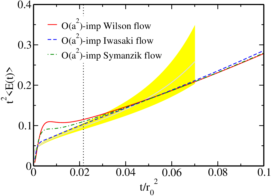


Figure 5 shows the dependence of calculated at . The three panels show results for unimproved flows (left), -imp flows (center), and the -imp Symanzik-like flow (right). For the unimproved case (left panel), the Wilson flow result is closest to the continuum perturbative calculation as same in the case of the Wilson gauge configurations. According to the size of tree-level discretization errors of summarized in Table 1, the three flow results move away from the continuum perturbative result.
| (Action) | () | [fm] | [fm] | ||
|---|---|---|---|---|---|
| 2.60 (IG) | 5.078(64) | 0.0985(12) | 2.36 | 100 | |
| 2.80 (IG) | 6.798(57) | 0.0736(6) | 2.36 | 100 | |
| 3.10 (IG) | 10.23(7) | 0.0489(3) | 2.35 | 100 | |
| 3.10 (IG) | 10.23(7) | 0.0489(3) | 1.56 | 100 |
In the center and right panels of Fig. 5, it is observed that our proposal of tree-level improvements works as well as the case of the Wilson gauge configurations (see Fig. 1 for comparison). Here we note that we omit the result obtained from another -imp flow (namely, the “positive rectangle flow”) in the right panel of Fig. 5. This is simply because the positive rectangle flow yields a negative value of in the entire positive flow time region () [29]. The numerical results for the -imp Symanzik flow (center panel) and the -imp Symanzik-like flow (right panel) mostly coincide since the coefficient of the -imp Symanzik flow is tiny, as shown in Table 1. Indeed, the rectangle coefficient () of the -imp Symanzik-like flow is quite close to the Symanzik action (). There is a neither qualitative nor quantitative difference between the results for the -imp Symanzik and -imp Symanzik-like flows. For these reasons, we hereafter focus on the -imp flows.
Let us take a closer look at the results for -imp flows (center panel). Among the three types of -imp flows, the -imp Iwasaki flow is closest to the continuum perturbation calculation, while the other flows largely overshoot the continuum counterpart in the relatively small- regime (). This is not observed in the case of the Wilson gauge configurations, where the three types of -imp flow mostly coincide near the continuum counterpart even in the small- regime up to . However, it should be remembered that the lattice-spacing dependence of the tree-level contribution is classified by powers of as defined in Eq. (8). In the strict sense, the tree-level improvement program proposed by Fodor et al. [13], where the tree-level contributions of are classified by powers of , is supposed to be valid only in the region of at (Iwasaki) or (Wilson).
In the large- regime (), the differences among the results from the three -imp flows gradually appear and also increase for a larger value of . As explained in Sec. III.1, the origin of these differences is the non-negligible corrections beyond the tree-level discretization effects. To see this point, we show the results from the three -imp flows at three different lattice spacings in Fig. 6. The left panel is for , the center one is for , and the left one is for . It is clear that the differences between these three -imp flows are diminished as we move from a coarser lattice spacing (left panel) to a finer lattice spacing (right panel).
In Fig. 7 we also plot the differences in the values of between -imp flows as functions of . The upper (lower) panel shows the difference between -imp Wilson and -imp Iwasaki (Symanzik) flows. Green dot-dashed, blue dashed, and red solid curves represent results at , 2.80, and 3.10. These figures clearly show that the differences appearing in both the smaller region () and larger region () stem from some discretization errors. Through a direct comparison of the results obtained in two different lattice volumes ( and ) at the finer lattice spacing (), we confirm that the finite-volume effects in calculations using the Iwasaki gauge configurations are also negligible in the range of , as depicted in Fig. 8.


IV Scaling behavior and continuum limit of action density
In this section, to see how much improvement we get from our proposal, we first show the behavior of as a function of . A similar plot was used in Ref. [2] for a discussion of the finite-lattice-spacing effects. Here, and are the Sommer scale [22] and the new reference scale defined in Eq. (3), respectively. Although we would like to discuss the discretization errors solely on the reference scale , the ratio also contains the finite-lattice-spacing effects on the Sommer scale, which is determined at finite lattice spacing.
For this reason, instead of , we will later discuss the scaling behavior of the dimensionless combination of with the QCD parameter in the scheme following the analysis of Ref. [30]. The parameter is determined through a matching between the lattice bare coupling to the running coupling with the help of perturbation theory. There is, at least, no power-like dependence on the lattice artifacts in the determination of . On the other hand, the choice of the smaller —which gives the higher energy scale —is desirable to ensure the applicability of a perturbative matching procedure.
In the previous section, we have found that the lattice discretization errors of the energy density around are well controlled by the or -imp flows. The corresponding is roughly 0.15, which is a factor of 2 reduction from the original choice of . In this study, we will later evaluate for and 0.3 as typical examples.
IV.1 The behavior of
In Ref. [2], the value of was evaluated from both the plaquette- and clover-type energy densities by using the Wilson flow. We here show the behavior of as a function of for several combinations of two gauge actions (WG and IG) and various flows in order to demonstrate the feasibility of our tree-level improvement proposal.
To evaluate the ratio , we use the values of determined in Refs. [23, 28]. Figure 9 just shows a feature of how much improvement has been achieved by tree-level and -imp flows. The results for are plotted against for various flows carried out on two types of gauge configurations (WG and IG). The two upper panels show the results obtained from unimproved flows, while the results for and -imp flows are presented in the two lower panels.
For the unimproved flows (upper panels), the results for both cases of (left) and 0.3 (right) very much depend on the choice of the gauge action and the flow. However, once any tree-level improvement is achieved, the differences among the different choices of the gauge action and the flow become significantly diminished. If one takes a closer look at the figures in the two lower panels of Fig. 9, the results calculated on the same gauge action (WG or IG) seem to be clustered while the gauge action dependence remains visible. However, we consider that the gauge action dependence would be partly attributed to the systematic uncertainties due to the scale setting by the Sommer scale, which was not directly determined in our numerical simulations. Furthermore, as described previously, the value of (which is determined in lattice QCD) itself receives the lattice discretization errors independently. Therefore, the ratio is not an appropriate quantity to discuss the lattice artifacts solely on . Instead of the Sommer scale, we will then use for the scale setting in the next section.


IV.2 Conversion to the scheme
The parameter is determined through a matching between the lattice bare coupling to the running coupling with help of perturbation theory. However, it is well known that the lattice perturbative expansions are poorly convergent. We thus introduce the tadpole-improved (TI) coupling, which is defined by
| (19) |
with
| (20) |
where and represent the expectation values of the the path-ordered plaquette and rectangle products of link variables, respectively [30, 31]. The tadpole-improved coupling can boost the slow convergence of a power series in the lattice bare coupling.
In order to evaluate the , let us consider a conversion from the boosted lattice scheme to the scheme as follows. The running coupling in the scheme, , is given by the following formula as a power series in the boosted coupling , up to :
| (21) | |||||
where and denote the one-loop and two-loop conversion variables with the first two coefficients of the function and being the universal coefficients in the pure Yang-Mills theory [30]. This conversion formula is fully determined by the NLO perturbation theory. However, the two-loop conversion variable, , is not known for the case of , since the three-loop term of the lattice function is not available for the RG-improved gauge action [32]. For the standard Wilson () and the Iwasaki () gauge actions, the currently known results for conversion variables in the tadpole-improved lattice scheme are summarized in Table 4.
We next choose the renormalization scale to remove the coefficient in Eq. (21) for its rapid convergence. To achieve this, the scale is set to
| (22) |
In this choice, the explicit dependence appears only at the level of in Eq. (21) with two-loop conversion variables. Therefore, the lattice discretization errors on the determination of become negligible in the weaker coupling region. This scale choice is called “method I” in Ref. [30] and reduces Eq. (21) to
| (23) |
which correspond to conversions from the boosted coupling to the coupling at one-loop (first line) and two-loop (second line) order of perturbation theory. To evaluate , we need to compute and numerically. We summarize our results for and in Table 5.
In this paper, we use the knowledge of the function at three-loop order for the evaluation of the parameter with a given coupling [30]. For the coupling at , we use the following formula for the parameter [30]:
| (24) |
with
where is the third coefficient of the function in the scheme[33]. We thus can determine the parameter through Eq.(24) by using the value of evaluated from either the one-loop or two-loop conversion formula in Eq. (23). The dimensionless combination of is finally obtained together with the numerically computed value of . If we stress that the one-loop (two-loop) formula in Eq. (23) is used for the conversion between two schemes, the resulting parameter in the scheme from Eq.(24) is denoted by ().


| Ref. | |||
|---|---|---|---|
| 0 | 0.0217565 | [30] | |
| N/A | [31] |
| (Action) | ||
|---|---|---|
| 5.96 (WG) | 0.589 1583(32) | — |
| 6.17 (WG) | 0.610 8670(14) | — |
| 6.42 (WG) | 0.632 2170(06) | — |
| 2.60 (IG) | 0.670 6232(15) | 0.452 8281(186) |
| 2.80 (IG) | 0.696 4317(61) | 0.490 0710(102) |
| 3.10 (IG) | 0.727 6215(21) | 0.536 2049(037) |
| type of calculation | type of extrapolation | ||||
|---|---|---|---|---|---|
| WG + -imp Wilson flow | 3 points linear | 0.1176(1) | 0.1339(1) | 0.1813(2) | 0.2064(2) |
| WG + -imp Wilson flow | 2 points linear | 0.1189(1) | 0.1347(2) | 0.1834(3) | 0.2079(4) |
| WG + -imp Wilson-like flow | 3 points linear | 0.1175(1) | 0.1337(1) | 0.1812(2) | 0.2063(3) |
| WG + -imp Wilson-like flow | 2 points linear | 0.1188(1) | 0.1347(2) | 0.1834(3) | 0.2080(4) |
| IG + -imp Iwasaki flow | 3 points linear | 0.1175(1) | N/A | 0.1832(2) | N/A |
| IG + -imp Iwasaki flow | 2 points linear | 0.1191(1) | N/A | 0.1853(3) | N/A |
IV.3 Scaling behavior of the parameter
In the following discussion, we use the one-loop formula in Eq. (23) to evaluate the value of in the scheme on both the Wilson and Iwasaki gauge configurations in order to treat them on the same footing, since the value of is not known for the Iwasaki gauge action, as mentioned earlier.
In Fig. 10, we plot the results for against from several combinations of two gauge actions and various flows for choices of (left panels) and (right panels), as in Fig. 9. The two upper panels show the results obtained by unimproved flows, while the two lower panels are for the results obtained by and -imp flows.
For the unimproved flows (upper panels), the results for both cases of (left) and 0.3 (right) very much depend on the choice of the gauge action and flow, similarly to the behavior of . However, the results given by all tree-level improved flows show a nearly perfect scaling behavior especially in the case of as a function of regardless of the types of gauge action and flow, unlike the behavior of . This indicates that the slight difference in the scaling behavior between the results obtained from WG and IG (which is found in Fig. 9) comes from the systematic uncertainties due to the scale setting by the Sommer scale.
For the case of , the scaling behavior becomes less prominent. The behavior of indeed reveals a weak dependence of the choice of the gauge action, while the scaling behavior among various tree-level improved flows on the same gauge configurations remains visible in the smaller region of . The violation of the scaling behavior of as a function of is mainly attributed to the fact that both Eqs. (23) and (24) are used beyond their applicability region. Indeed, is located in the larger region, where the renormalized coupling becomes large, as shown in Figs. 1, 2, 5, and 6.
Even for the case of , where the nearly perfect scaling is achieved, there is still a slight linear dependence of . However, if one reads off the slopes of the scaling behaviors from the lower left and right panels of Fig. 10, the slope for is less steep than for . The origin of linear scaling in terms of is undoubtedly related to the remnant corrections, as we will discuss in detail later.
We now consider the continuum limit of the values of . Among the various flow results, we focus on the tree-level improvement flows for the following specific cases (): the -imp Wilson flow on the Wilson gauge configurations, and the -imp Iwasaki flow on the Iwasaki gauge configurations.
For the continuum extrapolation, we simply adopt a linear form in terms of :
| (25) |
Making a least-squares fit to all three data points using Eq. (25), we get
| (26) | |||||
from the WG + -imp Wilson flow and
| (27) | |||||
from the IG + -imp Iwasaki flow. Even if we exclude the data point at the coarsest lattice spacing from the fit, the results are not much different, as summarized in Table 6. Clearly, for the smaller the resulting continuum value is stable against the choice of the gauge action and the flow. In this sense, after the tree-level improvement is achieved, the reference scale is much better controlled in comparison to the original one .
Recall that we do not take into account the possible large systematic error stemming from the uncertainty of determining . A precise determination of the continuum value of is the beyond scope of the present paper. The reason why we examine the scaling behavior of is that we would like to know the scaling property purely obtained from the reference scale without unknown systematic uncertainties of the lattice spacing discretization errors, arising from the introduction of other observables such as the Sommer scale .
Next, we examine the uncertainty of determining . For the Wilson gauge action, the fully NLO formula of the conversion from the boosted coupling to the coupling is known with the values of and as given in Table 4. Therefore, we would like to compare the results for , which are determined with both the one-loop and two-loop conversions of Eq. (23). When the two-loop conversion is used, we get
| (28) | |||||
which indicates that the uncertainties stemming from the scheme conversion on the coupling are estimated as about 12% for the determination of .
In Fig. 11, we plot the continuum extrapolated values of for various choices of as a function of in the range of . The results are obtained from data for the WG + -imp Wilson flow. The open circle symbols represent the results obtained when using the two-loop conversion, while the open diamond symbols represent the results obtained when using the one-loop conversion. Clearly, the difference between two results for each is considerably larger than their own statistical errors; meanwhile, the difference becomes more pronounced for larger values of .
Figure 11 also includes three results from the continuum perturbation theory. At a given scale , we evaluate the four-loop running coupling [26, 27] and then calculate the value of using the LO, NLO, and NNLO gradient flow formula of Eq. (2). The dashed, dot-dashed and solid curves represent the LO, NLO, and NNLO results. Our numerical results for from the lattice gradient flow are fairly consistent with the NNLO result from the perturbative gradient flow in the range of .


IV.4 Remnant corrections
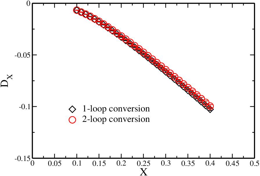
Finally, we discuss the origin of linear scaling in terms of observed in Fig. 10. The strength of the remnant scaling violation that is approximately proportional to can be read off from the dependence of the coefficient defined in the fitting form of Eq. (25). In Fig. 12, we show the dependence of the values of evaluated from both results when using the one-loop and two-loop conversions of Eq. (23). Although there are large uncertainties in the determination of due to the choice of the conversion formula (23), the differences in the slope coefficients obtained from two conversions are negligible especially for the smaller region.
Therefore, in the following discussion we use the results for obtained from the two-loop conversion with the WG + -imp Wilson flow. As briefly mentioned earlier, a nonzero value of for a given (which is associated with the scaling violation) could be mainly caused by non-negligible corrections beyond the tree-level discretization effects, as shown in Fig 12. It indeed seems that the value of goes to zero as decreases. If this is true, might vanish because of the asymptotic freedom () at high energies (). Therefore, we assume that is expressed by a power series in the running coupling at a scale of as follows:
| (29) |
where are the perturbative expansion coefficients. If the summation in the above equation starts at rather than , the origin of linear scaling is mainly associated with the remnant corrections, which arise beyond the tree level.
To verify this assumption, let us plot the ratio of to as a function of , as shown in Fig. 13. As for the value of , we consider two types of estimation. 1) One type is to use the perturbative four-loop expression for the running coupling with our numerical results for at a given . 2) Another type is to use the gradient flow (GF) coupling [34], which can be determined from the gradient flow formula of Eq. (2) with a given value of . In the latter, we adopt the NNLO formula, which yields a cubic equation with respect to at a fixed . We thus evaluate the ratio of to using the above two methods, as shown in Fig. 13.
The open square symbols represent the ratio given by the four-loop running coupling, while the open circle symbols are evaluated using the GF coupling. When , the cubic equation with respect to admits no feasible solution. For each case, we thus show 17 data points, which are in the range of . In the weaker coupling regime (), two results from different evaluations of the ratio overlap each other. Their eight or nine data points () start to show the expected weak coupling scaling behavior, which is almost linear in . To ensure this point, we have carried out the linear fit on the data set given by the GF coupling, which exhibits a milder dependence, using the following expression:
| (30) |
where and correspond to the coefficients for the first and second orders of in Eq. (29).
The stability of the fit results has been tested against the number of fitted data points. The best fit is drawn to fit eight data points, which are indicated by violet open circles in Fig. 13, with a reasonable value of . We then obtain the results
| (31) | |||||
which indicate that the remnant corrections are reasonably small in the weak-coupling regime. The fit result with one standard deviation is indicated by a red dashed line with a yellow shaded band in Fig. 13. From the above observation regarding , we conclude that the origin of linear scaling in terms of found in Fig. 10 is related to the remnant corrections, which are beyond the tree level. Although it is thus evident that the tree-level improvement program studied in this paper is not enough to eliminate all effects, the remnant corrections can be well under control even when using the simple method for the tree-level improvement.


V Summary
We have studied several types of tree-level improvement on the Yang-Mills gradient flow in order to reduce the lattice discretization errors on the expectation value of the action density , in line with Ref. [13]. For this purpose, the rectangle term was included in both the flow and gauge actions in the minimal way. We proposed a simple idea of achieving tree-level and improvements on , using the linear combination of two types of given by the plaquette- and clover-type definitions. To test our proposal, numerical simulations have also been performed with both the Wilson and Iwasaki gauge configurations generated at various lattice spacings.
Our numerical results have showed that tree-level lattice discretization errors on the quantity of are certainly controlled in the small- regime for up to by both tree-level - and -improved flows. On the other hand, the values of in the large- regime are different among the results given by different flow types, leading to the same improved flow up to either or at tree level.
In order to demonstrate the feasibility of our tree-level improvement proposal, we first plotted the behavior of as a function of in a similar manner as in Ref. [2]. However, the ratio also contains the discretization errors in the determination of in addition to those of the lattice gradient flow. We then studied the scaling behavior of the dimensionless combination of two scale parameters, , which is free in the weaker coupling regime from unknown systematic uncertainties regarding the lattice spacing discretization errors arising from the introduction of other observables on the lattice, such as the Sommer scale.
For the smaller , e.g., , once any tree-level improvement is achieved, shows a nearly perfect scaling behavior as a function of regardless the types of gauge action and flow. However, there is still a slight linear dependence of appearing in the cases of both - and -improved flows. On the other hand, for the larger , e.g., the original choice of , the behavior of reveals a weak dependence of the choice of the gauge action, while the scaling behavior among various tree-level improved flows on the same gauge configurations remains visible especially in the smaller region of .
All of the aforementioned features regarding the slight scaling violation and the gauge action dependence suggest that there still remain remnant corrections, which are beyond the tree level. Indeed, the origin of linear scaling in terms of found in is related to the remnant corrections, which can be read off from the dependence of the slope coefficient associated with the linear scaling.
Although it is evident that the tree-level improvement program studied in this paper is not enough to eliminate all effects, the remnant corrections can be well under control even with the simple method for the tree-level improvement. Once the tree-level and improvements are achieved, the resulting energy density becomes very close to the continuum one in the small- regime for up to . This offers an alternative reference scale with the smaller value of , such as . Indeed the continuum-extrapolated value of is in excellent agreement with the perturbative gradient flow result. On the other hand, it is observed that the original reference scale suffers from rather large errors when the lattice spacing is coarse, as large as fm.
Appendix A Comparison with the original proposal
Fodor et al. proposed a tree-level improvement of the action density [13] as defined in Eq. (18). In this appendix, we compare our results with results obtained from the original proposal. In Fig. 14, we show the results from the Iwasaki flow on the Wilson gauge configurations at three lattice spacings. This particular combination of the gauge action and the flow provides large differences between the original proposal and ours.
The three panels of Fig. 14 show the results calculated at (left), (center), and (right). The unimproved results for the Iwasaki flow with the clover-type action density are represented by the red dashed curve in each panel, while their improved results given by Eq. (18) are represented by the green dot-dashed curve in each panel. The blue solid curve in each panel represents our results obtained from the -imp Iwasaki flow.
Figure 14 shows that the improved action density defined in Eq. (18) does not efficiently improve the behavior of as a function of at the coarser lattice spacing, while our results from the -imp Iwasaki flow are much closer to the continuum perturbative calculation even in the relatively small- regime up to , which is beyond the boundary of asymptotic power-series expansions in terms of at .
The difference between the original proposal and ours becomes diminished as the lattice spacing decreases. Therefore, in results given by the original proposal the large deviation from the continuum perturbative calculation—which is found at the coarser lattice spacing—is certainly caused by the lattice discretization errors. Indeed, a simple division of the measured action density by the tree-level contribution could not eliminate the tree-level discretization corrections properly unless . This is the case when the large rectangle coefficient is chosen for the flow action. As shown in Secs. III and IV, our proposal does not have such a restriction on the value of , and can equally eliminate the tree-level discretization corrections for nonzero values of .
Acknowledgements.
We would like to thank the members of the FlowQCD Collaboration (T. Hatsuda, T. Iritani, E. Itou, M. Kitazawa and H. Suzuki) for helpful suggestions and fruitful discussions. This work is in part based on the Bridge++ code (http://bridge.kek.jp/Lattice-code/) and numerical calculations were partially carried out on supercomputer resources: SR16000 and XC40 at YTIP, Kyoto University, SR16000 under the Large-scale Simulation Program (No.15/16-02) at KEK, and LX406Re-2 under the HPCI Systems Research Projects (Project ID: hp160020) at Cyberscience Center, Tohoku University.References
- [1] R. Narayanan and H. Neuberger, JHEP 0603, 064 (2006).
- [2] M. Lüscher, JHEP 1008, 071 (2010) [Erratum-ibid. 1403, 092 (2014)].
- [3] S. Borsanyi et al., JHEP 1209, 010 (2012).
- [4] M. Asakawa, T. Hatsuda, T. Iritani, E. Itou, M. Kitazawa and H. Suzuki, arXiv:1503.06516 [hep-lat].
- [5] A. Ramos, JHEP 1411, 101 (2014).
- [6] H. Suzuki, PTEP 2013, no. 8, 083B03 (2013).
- [7] L. Del Debbio, A. Patella and A. Rago, JHEP 1311, 212 (2013).
- [8] M. Asakawa et al. [FlowQCD Collaboration], Phys. Rev. D 90, no. 1, 011501 (2014); Erratum: [Phys. Rev. D 92, no. 5, 059902 (2015)].
- [9] M. Kitazawa, T. Iritani, M. Asakawa, T. Hatsuda and H. Suzuki, Phys. Rev. D 94, no. 11, 114512 (2016).
- [10] Y. Taniguchi, K. Kanaya, H. Suzuki and T. Umeda, arXiv:1611.02411 [hep-lat].
- [11] Y. Taniguchi, S. Ejiri, K. Kanaya, M. Kitazawa, H. Suzuki, T. Umeda, R. Iwami and N. Wakabayashi, arXiv:1611.02413 [hep-lat].
- [12] M. Lüscher, PoS LATTICE 2013, 016 (2014).
- [13] Z. Fodor et al., JHEP 1409, 018 (2014).
- [14] A. Ramos and S. Sint, Eur. Phys. J. C 76, no. 1, 15 (2016).
- [15] FlowQCD Collaboration (private communication).
- [16] N. Kamata and S. Sasaki, PoS LATTICE 2015, 301 (2016).
- [17] Y. Iwasaki, arXiv:1111.7054 [hep-lat].
- [18] M. Lüscher and P. Weisz, JHEP 1102, 051 (2011).
- [19] R. V. Harlander and T. Neumann, JHEP 1606, 161 (2016).
- [20] M. Lüscher and P. Weisz, Commun. Math. Phys. 97, 59 (1985) Erratum: [Commun. Math. Phys. 98, 433 (1985)].
- [21] Please note that this linear combination is different from the tree-level “operator,” , proposed by Ramos and Sint [14].
- [22] R. Sommer, Nucl. Phys. B 411, 839 (1994).
- [23] M. Guagnelli et al. [ALPHA Collaboration], Nucl. Phys. B 535, 389 (1998).
- [24] N. Cabibbo and E. Marinari, Phys. Lett. B 119, 387 (1982).
- [25] M. Creutz, Phys. Rev. D 36, 515 (1987).
- [26] T. van Ritbergen, J. A. M. Vermaseren and S. A. Larin, Phys. Lett. B 400, 379 (1997).
- [27] M. Czakon, Nucl. Phys. B 710 (2005) 485.
- [28] S. Takeda et al., Phys. Rev. D 70, 074510 (2004).
- [29] Note that although the positive rectangle flow yields positive values of and , the -improved combination of Eq.(11) makes negative.
- [30] M. Göckeler, R. Horsley, A. C. Irving, D. Pleiter, P. E. L. Rakow, G. Schierholz and H. Stuben, Phys. Rev. D 73, 014513 (2006).
- [31] A. Ali Khan et al. [CP-PACS Collaboration], Phys. Rev. D 64, 114506 (2001).
- [32] A. Skouroupathis and H. Panagopoulos, Phys. Rev. D 76, 114514 (2007).
- [33] In the first version of this paper, we simply used the standard two-loop formula for the parameter, instead of Eq. (24). However, the determination of the two-loop conversion variable requires the three-loop function coefficients in two schemes [30]. We thus update the analysis using the three-loop formula (24) to ensure the two-loop accuracy on the parameter in the case of the two-loop conversion.
- [34] Z. Fodor, K. Holland, J. Kuti, D. Nogradi and C. H. Wong, JHEP 1211, 007 (2012).