跳到论文正文
W Papers独立论文阅读器 arXiv:1609.07073 论文正文 计算阅读时间 · 0%
引用这篇论文根据当前论文元数据生成,正式投稿前建议核对。


License: arXiv.org perpetual non-exclusive license
arXiv:1609.07073v3 [cond-mat.stat-mech] 08 Apr 2018

Unattainability of Carnot efficiency in thermal motors:
Coarse-graining and entropy production of Feynman-Smoluchowski ratchet

Yohei Nakayama Affiliation: Department of Physics, Chuo University, Tokyo 112-8551, Japan Email: nakayama@phys.chuo-u.ac.jp    Kyogo Kawaguchi Affiliation: Department of Systems Biology, Harvard Medical School, Boston, MA02115, USA Email: Kyogo_Kawaguchi@hms.harvard.edu    Naoko Nakagawa Affiliation: College of Science, Ibaraki University, Ibaraki 310-8512, Japan Email: naoko.nakagawa.phys@vc.ibaraki.ac.jp
August 24, 2026
Abstract

We revisit and analyze the thermodynamic efficiency of the Feynman-Smoluchowski (FS) ratchet, a classical thought experiment describing an autonomous heat-work converter. Starting from the full kinetics of the FS ratchet and deriving the exact forms of the hidden dissipations resulting from coarse-graining, we restate the historical controversy over its thermodynamic efficiency. The existence of hidden entropy productions implies that the standard framework of stochastic thermodynamics applied to the coarse-grained descriptions fails in capturing the dissipative feature of the system. In response to this problem, we explore an extended framework of stochastic thermodynamics to reconstruct the hidden entropy production from the coarse-grained dynamics. The approach serves as a key example of how we can systematically address the problem of thermodynamic efficiency in a multi-variable fluctuating non-equilibrium system.

I Introduction

The framework of stochastic thermodynamics has not only allowed experimental characterization of small thermodynamic systems [1], but has also established a unified scheme to address fundamental questions in thermodynamics. Identities and inequalities formulated for general stochastic dynamics have been given thermodynamical interpretations such as the second law [2, 3, 4], role of information feedback [5, 1], bound on efficiencies of engines at finite time operations [6, 7], and laws extended to nonequilibrium setups [8, 9, 10].

The crucial concept behind the developments in stochastic thermodynamics is the entropy production, which is typically introduced through local detailed balance using the logarithmic ratio of transition probabilities [11]. This quantity is equivalent, at least in several models, to the energy exchanged with the heat bath divided by the temperature of the bath [12], and satisfies the second law-like inequality. Recent works, however, have clarified that fluctuating nonequilibrium systems can carry hidden entropy productions [13, 14, 15, 16, 17, 18, 19, 20, 21, 22, 23, 24], and even under the properly-controlled limit of coarse-graining the coarse-grained model may not preserve the thermodynamic properties of the original system [14, 16, 20, 25].

In this paper, we focus on the analysis of the Feynman-Smoluchowski (FS) ratchet (Figure 1a) [26] as a model case to understand how the thermodynamic efficiency can seemlingly change according to the different coarse-grained descriptions of the dynamics.

Refer to caption(a) Models-0,1,4(b) Models-2,3(c)(d)
Figure 1: Schematics of the FS ratchet and its coarse-grained descriptions. (a) In Models-0, 1 and 4, the FS ratchet consists of a vane, a gear and a pawl. A spring presses the pawl against the gear, and an external load applies torque to the axle. The vane and pawl are attached to different heat baths. (b) In Models-2 and 3, Langevin equations with the effective mechanical potential, Ueff​(θ)U_{\mathrm{eff}}(\theta), inhomogeneous friction, 𝒢⁡(θ)\mathcal{G}(\theta), and temperature, Teff​(θ)T_{\mathrm{eff}}(\theta), describe the dynamics of the FS ratchet. (c) The scheme of coarse-graining and the degrees of freedom in Models-0, 1, 2, 3, 4 and 5. (d) Langevin equation with stochastic switching between the two heat baths (Model-6).

The FS ratchet is one of the most celebrated thought experiments in thermodynamics, where there has been a controversy over its thermodynamic efficiency. The FS ratchet, due to its asymmetric design, may appear as if it can convert the thermal fluctuation of a single heat bath into work by unidirectional rotation, violating the second law of thermodynamics. After Smoluchowski showed that there is no rotation and extracted work if the FS ratchet is placed in an isothermal environment [27], in The Feynman Lectures on Physics [26], Feynman considered whether it is possible for the ratchet to operate as a Carnot efficient engine. It was claimed, based on the analysis of a simplified discrete-stepping model, that the ratchet may attain Carnot efficiency at the stalled state between two heat baths with different temperatures.

Parrondo and Español, however, critisized Feynman’s argument and pointed out that the momentum variable is non-negligible for the dissipation in the FS ratchet by using a different method of simplifying the model [28]. In addition, the unattainability of Carnot efficiency was established in another autonomous Brownian heat engine, Büttiker-Landauer (BL) motor [29, 30, 31], which is a model that has been thought to be closely related to the FS ratchet. These studies have thus formed a consensus that the FS ratchet cannot attain Carnot efficiency [32, 33, 34].

Thermodynamic efficiencies in coarse-grained models are not only a theoretical concern but also important in the interpretation of experimental data, since the measurements are typically restricted to a small set of slow variables. The potential existence of hidden entropy productions (i.e., dissipation owing to the unobserved variables) will make it virtually impossible to draw any conclusions about thermodynamic efficiency in a nonequilibrium small system experiment. Therefore, it is of interest to extend the framework of stochastic thermodynamics to be able to re-interpret the coarse-grained data in order to obtain the original thermodynamic properties.

Here we aim to provide a unified understanding and a workaround to the FS ratchet problem, through a systematic procedure of coarse-graining which does not involving any empirical simplifications. We derive the coarse-grained descriptions of the original FS ratchet including the previously known models [35, 36, 37, 38, 39] together with new models. We then ask how the entropy productions may differ in the series of models by obtaining the explicit expressions for the hidden entropy productions, and discuss their relations to the previous arguments on the controversial thermodynamic efficiencies. Finding that most of the coarse-grained dynamics do not preserve the thermodynamic property of the original FS ratchet, we further explore and find a way to quantify the hidden dissipation based on a limited number of coarse-grained observables.

This paper is organized as follows. In Sec. II we introduce the original FS ratchet model (Model-0). In Sec. III the coarse-grained descriptions (Models-2,3 and 5) are derived by taking the time-scale separation limits. In Sec. IV we calculate the behavior of the dissipation through the framework of stochastic thermodynamics, in the limits where the coarse-grained descriptions are obtained. We derive the explicit forms of hidden entropy productions as the first main result of the paper. In addition, we clarify that what Feynman did can be regarded as applying stochastic thermodynamics to the coarse-grained description. In Sec. V we present the results of numerical simulations which clarify the impact of hidden entropy production on the thermodynamic efficiencies (Figure 6). These results confirm that although the kinetics of the FS ratchet can be coarse-grained systematically, most of the coarse-grained models do not reproduce the entropy production of the original system. In Sec. VI we describe our proposal of a workaround to the problem of hidden entropy production by demonstrating that even when using the coarse-grained variables, the fine-grained entropy production can be reconstructed by the decomposition of the Langevin dynamics (Model-6). In Sec. VII we give concluding remarks. Some technical details are described in Appendices.

II Setup

As shown in Figure 1a, the FS ratchet consists of a vane and a gear connected by a rigid axle, and a pawl meshing with the gear. A spring pushes the pawl against the gear. The vane and the pawl are in contact with different heat baths with temperatures ThT_{h} and TcT_{c}. An external load couples with the axle, and applies a constant torque, ff. By assuming the interaction between the pawl and the gear to be mechanical, the equations of motion for the angle θ\theta of the coaxial vane and gear and the height xx of the pawl reads

θ˙=Πm,Π˙=−Γm​Π+f−∂U⁡(θ,x)∂θ+2​Γ​Th​ξ,x˙=pmx,p˙=−γmx​p−∂U⁡(θ,x)∂x+2​γ​Tc​ζ,\displaystyle\begin{split}\dot{\theta}&=\frac{\Pi}{m},\\ \dot{\Pi}&=-\frac{\Gamma}{m}\Pi+f-\frac{\partial U(\theta,x)}{{\partial\theta}}+\sqrt{2\Gamma T_{h}}\xi,\\ \dot{x}&=\frac{p}{m_{x}},\\ \dot{p}&=-\frac{\gamma}{m_{x}}p-\frac{\partial U(\theta,x)}{{\partial x}}+\sqrt{2\gamma T_{c}}\zeta,\end{split} (Model-0)

where Π\Pi and pp are the momentum conjugated to θ\theta and xx, respectively. Here, mm is the corresponding moment of inertia, and mxm_{x} is the mass of the pawl. We take Langevin heat baths where Γ\Gamma and γ\gamma are the viscous frictional coefficients. ξ\xi and ζ\zeta are independent white Gaussian noises with zero means and unit variances. The Boltzmann constant is set to unity.

In a straightforward manner, we may obtain a coarse-grained description,

θ˙=Πm,Π˙=−Γm​Π+f−∂U⁡(θ,x)∂θ+2​Γ​Th​ξ,γ​x˙=−∂U⁡(θ,x)∂x+2​γ​Tc​ζ~,\displaystyle\begin{split}\dot{\theta}&=\frac{\Pi}{m},\\ \dot{\Pi}&=-\frac{\Gamma}{m}\Pi+f-\frac{\partial U(\theta,x)}{\partial\theta}+\sqrt{2\Gamma T_{h}}\xi,\\ \gamma\dot{x}&=-\frac{\partial U(\theta,x)}{\partial x}+\sqrt{2\gamma T_{c}}\tilde{\zeta},\end{split} (Model-1)

where the momentum degree of freedom, pp, is eliminated by considering the overdamped limit for the pawl. The symbol ζ~\tilde{\zeta} is an independent white Gaussian noise with zero mean and unit variance.

We assume the mechanical potential

U⁡(θ,x)=U0​(x)+UI​(x−ϕ⁡(θ)),\displaystyle U(\theta,x)=U_{0}(x)+U_{I}(x-\phi(\theta)), (1)

where U0​(x)U_{0}(x) is the elastic potential of the spring attached to the pawl and UI​(x−ϕ​(θ))U_{I}(x-\phi(\theta)) is the trapping potential between the tip of pawl and the surface of gear. ϕ⁡(θ)\phi(\theta) is a periodic function which represents the shape of gear, with the period LL.

III Coarse-graining

We here explicitly derive the coarse-grained descriptions of Model-1 by taking the limits where the time-scales of the variables are separated.This is in contrast to the approaches taken for example in [26] where the discrete stepping model and the BL motor were introduced on the basis of phenomenological arguments. We start from Model-1 and consider two limits, a “tightly confined limit” and a “overdamped limit”, where xx and Π\Pi are eliminated, respectively. Through this two-step coarse-graining, we arrive at a closed equation of motion for θ\theta. We note that the order of elimination of xx and Π\Pi matters. As summarized in Figure 2, we find that taking the tightly-confined limit first will result in a different model to when the overdamped limit is taken first (Model-3 vs Model-5).

Refer to caption
Figure 2: A complete picture of the routes of coarse-graining. The arrows represent the processes of coarse-graining where the necessity limit conditions to carry out the coarse-graining are specified. The yellow ones represent the coarse-graining processes derived in this paper, and the green ones correspond to the trivial coarse-graining eliminating the momentum variable attached to the isothermal environment. τx=Lx2​γ/Tc\tau_{x}=L_{x}^{2}\gamma/T_{c} and τΠ=m/Γ\tau_{\Pi}=m/\Gamma are the time scales of the pawl and momentum degree of freedom, respectively, and τ\tau is a time scale representing the other time scales of the system.

Hereafter, we denote the time scale of the relaxation in the trapping potential as τx:=Lx2​γ/Tc\tau_{x}:=L_{x}^{2}\gamma/T_{c} with the length scale LxL_{x} of the trapping potential. The time scale for the relaxation of the momentum of the vane and the gear is τΠ=m/Γ\tau_{\Pi}=m/\Gamma. We assume the other time scales to be of the same order, represented by τ\tau. In order to satisfy this assumption, we fix the functional forms of ϕ⁡(θ)\phi(\theta) and U0​(x)U_{0}(x) and the ratios Γ/γ\Gamma/\gamma, Tc/ThT_{c}/T_{h} and f​L/ThfL/T_{h}. We are interested in the cases where τx\tau_{x} and τΠ\tau_{\Pi} are separated from τ\tau.

Here we note on why we chose the interaction between the tip of the pawl and the surface of the gear UI​(x−ϕ​(θ))U_{I}(x-\phi(\theta)) as a trapping potential. In the original FS ratchet, this interaction was a hard-core repulsion, so the tight confinement of the pawl could only be realized by increasing the force exerted by the spring [U0​(x)U_{0}(x)], since the length scale of the confinement is proportional to Th/[∂U⁡(θ,x)/∂x]T_{h}/[\partial U(\theta,x)/\partial x]. However, the energy required to lift the pawl becomes larger than the thermal energy when increasing the spring force, which means that the FS ratchet will stop rotating in this limit. By introducing UI​(x−ϕ​(θ))U_{I}(x-\phi(\theta)) as a trapping potential, we may take the the tightly confined limit by keeping the height of the potential barrier constant. This modification to the original dynamics is the key in conducting the following coarse-graining procedures.

We mainly conduct coarse-graining in terms of the master equation, i.e., partial differential equation satisfied by probability densities. The master equation for Model-1 reads

∂P⁡(θ,Π,x)∂t=−∂∂θ​[Πm​P​(θ,Π,x)]\displaystyle\frac{\partial P(\theta,\Pi,x)}{{\partial t}}=-\frac{\partial}{{\partial\theta}}\left[\frac{\Pi}{m}P(\theta,\Pi,x)\right]
−∂∂Π​[(−Γm​Π+f−∂U⁡(θ,x)∂θ)​P​(θ,Π,x)−Γ​Th​∂P⁡(θ,Π,x)∂Π]\displaystyle-\frac{\partial}{{\partial\Pi}}\left[\left(-\frac{\Gamma}{m}\Pi+f-\frac{\partial U(\theta,x)}{{\partial\theta}}\right)P(\theta,\Pi,x)-\Gamma T_{h}\frac{\partial P(\theta,\Pi,x)}{{\partial\Pi}}\right]
−∂∂x​(−1γ​∂U⁡(θ,x)∂x​P​(θ,Π,x)−Tcγ​∂P⁡(θ,Π,x)∂x).\displaystyle-\frac{\partial}{{\partial x}}\left(-\frac{1}{\gamma}\frac{\partial U(\theta,x)}{{\partial x}}P(\theta,\Pi,x)-\frac{T_{c}}{\gamma}\frac{\partial P(\theta,\Pi,x)}{{\partial x}}\right). (2)

Here, P⁡(θ,Π,x)P(\theta,\Pi,x) represents the joint probability density of θ,Π\theta,\Pi and xx.

III.1 Coarse-grained Description at Tightly Confined Limit

We first consider the limit where the tip of the pawl is tightly confined to the surface of the gear. In this limit, τx\tau_{x} is assumed to be separated from τΠ\tau_{\Pi} and τ\tau. Assuming that the ratio τΠ/τ\tau_{\Pi}/\tau is fixed in this section, we introduce a small parameter representing the separation of time scales, ε:=τx/τΠ∼τx/τ\varepsilon:=\tau_{x}/\tau_{\Pi}\sim\tau_{x}/\tau. Here, we summarize the derivation of the coarse-grained description, and give the details in Appendix A-A.1.

In this tightly confined limit, the height of the pawl xx is eliminated as the fast variable. Therefore, the coarse-grained dynamics is described by the master equation for the joint probability density, P⁡(θ,Π)=∫d​x​P​(θ,Π,x)P(\theta,\Pi)=\int dxP(\theta,\Pi,x). Throughout this paper, the integrals with respect to θ,Π\theta,\Pi and xx are taken over the domain of integrand. The time derivative of P⁡(θ,Π)P(\theta,\Pi) is obtained by integrating Eq. (2) with respect to xx:

∂P⁡(θ,Π)∂t=\displaystyle\frac{\partial P(\theta,\Pi)}{{\partial t}}= −∂∂θ​[Πm​P​(θ,Π)]\displaystyle-\frac{\partial}{{\partial\theta}}\left[\frac{\Pi}{m}P(\theta,\Pi)\right]
−∂∂Π​[(−Γm​Π+f)​P​(θ,Π)−Γ​Th​∂P⁡(θ,Π)∂Π]\displaystyle-\frac{\partial}{{\partial\Pi}}\left[\left(-\frac{\Gamma}{m}\Pi+f\right)P(\theta,\Pi)-\Gamma T_{h}\frac{\partial P(\theta,\Pi)}{{\partial\Pi}}\right]
−∂∂Π[−∫dx∂U⁡(θ,x)∂θP(θ,Π,x)].\displaystyle-\frac{\partial}{{\partial\Pi}}\left[-\int dx\frac{\partial U(\theta,x)}{{\partial\theta}}P(\theta,\Pi,x)\right]. (3)

The closed equation for P⁡(θ,Π)P(\theta,\Pi) is obtained by evaluating the last line of Eq. (3) in the limit of ε→0\varepsilon\to 0. Employing the singular perturbation theory to avoid the divergence caused by the secular terms, we obtain

∂P⁡(θ,Π)∂t=−∂∂θ​[Πm​P​(θ,Π)]\displaystyle\frac{\partial P(\theta,\Pi)}{{\partial t}}=-\frac{\partial}{{\partial\theta}}\left[\frac{\Pi}{m}P(\theta,\Pi)\right]
−∂∂Π​[−𝒢⁡(θ)m​Π−∂Ueff​(θ)∂θ+f−𝒢⁡(θ)​Teff​(θ)​∂∂Π]​P​(θ,Π),\displaystyle-\frac{\partial}{{\partial\Pi}}\left[-\frac{\mathcal{G}(\theta)}{m}\Pi-\frac{\partial U_{\mathrm{eff}}(\theta)}{{\partial\theta}}+f-\mathcal{G}(\theta)T_{\mathrm{eff}}(\theta)\frac{\partial}{{\partial\Pi}}\right]P(\theta,\Pi), (4)

which is the Kramers equation. Here, Ueff​(θ)U_{\mathrm{eff}}(\theta), 𝒢⁡(θ)\mathcal{G}(\theta) and Teff​(θ)T_{\mathrm{eff}}(\theta) are the effective potential, the effective frictional coefficient and the effective temperature:

Ueff​(θ)\displaystyle U_{\mathrm{eff}}(\theta) =U0​(ϕ​(θ)),\displaystyle=U_{0}(\phi(\theta)), (5)
𝒢⁡(θ)\displaystyle\mathcal{G}(\theta) =Γ+γ​ϕ′​(θ)2,\displaystyle=\Gamma+\gamma\phi^{\prime}(\theta)^{2}, (6)
Teff​(θ)\displaystyle T_{\mathrm{eff}}(\theta) =Γ​Th+γ​ϕ′​(θ)2​TcΓ+γ​ϕ′​(θ)2.\displaystyle=\frac{\Gamma T_{h}+\gamma\phi^{\prime}(\theta)^{2}T_{c}}{\Gamma+\gamma\phi^{\prime}(\theta)^{2}}. (7)

The master equation (4) is equivalent to the Langevin equation

θ˙=Πm,Π˙=−𝒢⁡(θ)m​Π+f−∂Ueff​(θ)∂θ+2​𝒢​(θ)​Teff​(θ)​Ξ,\displaystyle\begin{split}\dot{\theta}&=\frac{\Pi}{m},\\ \dot{\Pi}&=-\frac{\mathcal{G}(\theta)}{m}\Pi+f-\frac{\partial U_{\mathrm{eff}}(\theta)}{\partial\theta}+\sqrt{2\mathcal{G}(\theta)T_{\mathrm{eff}}(\theta)}\Xi,\end{split} (Model-2)

where Ξ\Xi is a white Gaussian noise with zero mean and unit variance. Model-2 describes the Brownian motion of a single degree of freedom under the effective potential, frictional coefficient, and temperature (Figure 1b), which is known as the Büttiker-Landauer motor [35].

III.2 Quick Derivation of Model-2

We here give a quick derivation of Model-2 in the special case where we set U⁡(θ,x)=k​x2/2+λ​[x−ϕ⁡(θ)]2/2U(\theta,x)=kx^{2}/2+\lambda[x-\phi(\theta)]^{2}/2, based on a temporal coarse-graining method [40, 41]. The details will be given in Appendix A-A.2. Since the equation of motion

γ​x˙\displaystyle\gamma\dot{x} =−(k+λ)​x+λ​ϕ​(θ)+2​γ​Tc​ζ~,\displaystyle=-(k+\lambda)x+\lambda\phi(\theta)+\sqrt{2\gamma T_{c}}\tilde{\zeta}, (8)

is linear in xx, we may formally solve xx as the functional of ϕ⁡(θ)\phi(\theta) and ζ~\tilde{\zeta}, and eliminate xx by substituting the formal solution of xx into the equation of motion of Π\Pi:

Π˙t=\displaystyle\dot{\Pi}_{t}= −Γm​Πt+f+λ​ϕ′​(θt)​[−kk+λ​ϕ​(θt)−γ​λ(k+λ)2​ϕ′​(θt)​Πtm]\displaystyle-\frac{\Gamma}{m}\Pi_{t}+f+\lambda\phi^{\prime}(\theta_{t})\left[-\frac{k}{k+\lambda}\phi(\theta_{t})-\frac{\gamma\lambda}{(k+\lambda)^{2}}\phi^{\prime}(\theta_{t})\frac{\Pi_{t}}{m}\right]
+λ​ϕ′​(θt)​2​γ​Tcγ∫−∞tdt′e−k+λγ​(t−t′)ζ~t′+2​Γ​Thξt,\displaystyle+\frac{\lambda\phi^{\prime}(\theta_{t})\sqrt{2\gamma T_{c}}}{\gamma}\int_{-\infty}^{t}dt^{\prime}e^{-\frac{k+\lambda}{\gamma}(t-t^{\prime})}\tilde{\zeta}_{t^{\prime}}+\sqrt{2\Gamma T_{h}}\xi_{t}, (9)

where we explicitly show the time-dependence of the variables as the subscript. Note that Eq. (9) describes a non-Markovian dynamics with colored noise. The Markovian property is recovered in the limit of ε=τx/τΠ→0\varepsilon=\tau_{x}/\tau_{\Pi}\to 0. In this limit, we may introduce a time interval Δ​t\Delta t, which is shorter than τΠ\tau_{\Pi} and τ\tau, but longer than τx=γ/(k+λ)\tau_{x}=\gamma/(k+\lambda). By integrating Eq. (9) over the time interval Δ​t\Delta t and taking the limit of ε→0\varepsilon\to 0, we obtain Model-2.

III.3 Coarse-grained Description at Overdamped Limit

Next, we discuss the overdamped limit. In this limit τΠ=m/Γ\tau_{\Pi}=m/\Gamma is separated from the other time scales represented by τ\tau. The underdamped Brownian motion corresponding to Model-2 can be coarse-grained to an overdamped Langevin equation [42, 43]:

𝒢⁡(θ)⊙θ˙=\displaystyle\mathcal{G}(\theta)\odot\dot{\theta}= f−∂Ueff​(θ)∂θ+2​𝒢​(θ)⊙Teff​(θ)⋅Ξ~,\displaystyle f-\frac{\partial U_{\mathrm{eff}}(\theta)}{\partial\theta}+\sqrt{2\mathcal{G}(\theta)}\odot\sqrt{T_{\mathrm{eff}}(\theta)}\cdot\tilde{\Xi}, (Model-3)

where Ξ~\tilde{\Xi} is a white Gaussian noise with zero mean and unit variance. The symbols ⋅\cdot and ⊙\odot indicate the product in the sense of Itô and anti-Itô, respectively, which specify the evaluation of the quantity on the left:

2​𝒢​(θ)⊙Teff​(θ)⋅Ξ~=limδ​t→02​𝒢​(θt+δ​t)​Teff​(θt)​1δ​t​∫tt+δ​tΞ~s​𝑑s.\displaystyle\sqrt{2\mathcal{G}(\theta)}\odot\sqrt{T_{\mathrm{eff}}(\theta)}\cdot\tilde{\Xi}=\lim_{\delta t\to 0}\sqrt{2\mathcal{G}(\theta_{t+\delta t})T_{\mathrm{eff}}(\theta_{t})}\frac{1}{\delta t}\int_{t}^{t+\delta t}\!\!\!\!\!\tilde{\Xi}_{s}ds. (10)

Model-3 is a generalized version of the Büttiker-Landauer motor to the case of θ\theta-dependent friction. The net velocity of rotation of this motor is obtained as [35]

⟨θ˙⟩=L⁡[1−exp⁡(−L​Δ)]∫0Ld​y​exp​[−ψ⁡(y)]​∫yy+Ld​y′​exp​[ψ⁡(y′)]​𝒢​(y′)/Teff​(y′),\displaystyle\langle\dot{\theta}\rangle=\frac{L[1-\exp(-L\Delta)]}{\int_{0}^{L}dy\exp[-\psi(y)]\int_{y}^{y+L}dy^{\prime}\exp[\psi(y^{\prime})]\mathcal{G}(y^{\prime})/T_{\mathrm{eff}}(y^{\prime})}, (11)

where ⟨⋅⟩\langle\cdot\rangle represents the steady-state ensemble average and

ψ⁡(y)\displaystyle\psi(y) :=∫yd​y′​f−Ueff′​(y′)−Teff′​(y′)Teff​(y′),\displaystyle:=\int^{y}dy^{\prime}\frac{f-U^{\prime}_{\mathrm{eff}}(y^{\prime})-T^{\prime}_{\mathrm{eff}}(y^{\prime})}{T_{\mathrm{eff}}(y^{\prime})}, (12)
Δ\displaystyle\Delta :=ψ⁡(y)−ψ⁡(y+L).\displaystyle:=\psi(y)-\psi(y+L). (13)

Equation (11) indicates that there is unidirectional motion if Δ≠0\Delta\neq 0. The system works as a Brownian heat engine when the rotation is opposite to the direction of the constant torque: ⟨θ˙⟩<0\langle\dot{\theta}\rangle<0 (Δ<0)(\Delta<0) when f>0f>0. In Appendix A-A.3, we present the derivation of Model-3 based on the singular perturbation theory [16].

III.4 Other Routes of Coarse-graining

As shown in Figure 2, there is another path to obtain the closed equation of motion for θ\theta; we can take the overdamped limit before the tightly confined limit. In a straightforward manner, we obtain a coarse-grained description of Model-1

Γ​θ˙=f−∂U⁡(θ,x)∂θ+2​Γ​Th​ξ~,γ​x˙=−∂U⁡(θ,x)∂x+2​γ​Tc​ζ~,\displaystyle\begin{split}\Gamma\dot{\theta}=&f-\frac{\partial U(\theta,x)}{{\partial\theta}}+\sqrt{2\Gamma T_{h}}\tilde{\xi},\\ \gamma\dot{x}&=-\frac{\partial U(\theta,x)}{{\partial x}}+\sqrt{2\gamma T_{c}}\tilde{\zeta},\end{split} (Model-4)

which is equivalent to the master equation:

∂P⁡(θ,x)∂t=\displaystyle\frac{\partial P(\theta,x)}{{\partial t}}= −∂∂θ​[1Γ​(f−∂U⁡(θ,x)∂θ)​P​(θ,x)−ThΓ​∂P⁡(θ,x)∂θ]\displaystyle-\frac{\partial}{{\partial\theta}}\left[\frac{1}{\Gamma}\left(f-\frac{\partial U(\theta,x)}{{\partial\theta}}\right)P(\theta,x)-\frac{T_{h}}{\Gamma}\frac{\partial P(\theta,x)}{{\partial\theta}}\right]
−∂∂x​[−1γ​∂U⁡(θ,x)∂θ​P​(θ,x)−Tcγ​∂P⁡(θ,x)∂x].\displaystyle-\frac{\partial}{{\partial x}}\left[-\frac{1}{\gamma}\frac{\partial U(\theta,x)}{{\partial\theta}}P(\theta,x)-\frac{T_{c}}{\gamma}\frac{\partial P(\theta,x)}{{\partial x}}\right]. (14)

Here, ξ~\tilde{\xi} is an independent white Gaussian noise with zero mean and unit variance. Model-4 may also be obtained from Model-0 by taking the overdamped limit for the vane and the gear first (Figure 2). This type of model has also been analyzed in the context of the FS ratchet [37, 38, 39].

The time evolution of P⁡(θ)=∫d​x​P​(θ,x)P(\theta)=\int dxP(\theta,x) is obtained by taking the tightly-confined limit in Eq. (14). In the form of the Langevin equation, the coarse-grained description is obtained as

𝒢⁡(θ)⊙θ˙=f−∂Ueff​(θ)∂θ−∂ln⁡𝒢⁡(θ)∂θ​(Th−Tc)+2​𝒢​(θ)⊙Teff​(θ)⋅Ξ^.\displaystyle\begin{split}\mathcal{G}(\theta)\odot\dot{\theta}=&f-\frac{\partial U_{\mathrm{eff}}(\theta)}{{\partial\theta}}-\frac{\partial\ln\mathcal{G}(\theta)}{{\partial\theta}}(T_{h}-T_{c})\\ &+\sqrt{2\mathcal{G}(\theta)}\odot\sqrt{T_{\mathrm{eff}}(\theta)}\cdot\hat{\Xi}.\end{split} (Model-5)

where Ξ^\hat{\Xi} is a white Gaussian noise with zero mean and unit variance. Unidirectional motion is driven by the same mechanism as Model-3. The details of the derivation are given in Appendix A-A.4.

Model-3 and Model-5 are similar but slightly different; there is an extra term in Model-5 that vanishes when Th=TcT_{h}=T_{c} but affects the average velocity when Th≠TcT_{h}\neq T_{c}. Formally, this means that the two limits, τx≪τΠ≪τ\tau_{x}\ll\tau_{\Pi}\ll\tau (Model-3) and τΠ≪τx≪τ\tau_{\Pi}\ll\tau_{x}\ll\tau (Model-5) are different under a non-equilibrium setup.

We here note on some of the previous works related to the coarse-graining of FS ratchet-like dynamics. In [44], the authors coarse-grained Model-4 based on phenomenlogical arguments, and correctly obtained the effective potential and temperature [Eqs. (5,7)]. However, they did not arrive at the inhomogeneous friction [Eqs. (6)] and the force proportional to temperature-difference (the third term of the right hand side of Model-5). In [45], a similar attempt was made to obtain a phenomenological model by neglecting the temporal correlation of the fast variable, which resulted in an unphysical model that does not satisfy the fluctuation-dissipation relation. In [36], Millonas considered a non-equilibrium bath variable (xx in our model) that couples to a motor, and essentially obtained all of Eqs. (5-7). The aspects of dissipation and thermodynamic efficiency, however, were not discussed.

IV Stochastic Thermodynamics of Feynman-Smoluchowski Ratchet

We here discuss the thermodynamic properties of the FS ratchet by applying the framework of stochastic thermodynamics. We first describe the entropy production for each model, and then take the coarse-graining limits in each case to see if there is descrepancy (i.e., hidden entropy production) between the different scales of descriptions.

IV.1 Entropy Production Rates

The standard prescription of stochastic thermodynamics [11] connects the entropy production rate in the heat baths with the transition probabilities of the model. The entropy production rates for the models are written as

σ1(θt′,Πt′,xt′|θt,Πt,xt):=\displaystyle\sigma_{1}(\theta_{t^{\prime}},\Pi_{t^{\prime}},x_{t^{\prime}}|\theta_{t},\Pi_{t},x_{t}):= 1t′−t​ln⁡W1(θt′,Πt′,xt′|θt,Πt,xt)W1(θt,−Πt,xt|θt′,−Πt′,xt′)\displaystyle\frac{1}{t^{\prime}-t}\ln\frac{W_{1}(\theta_{t^{\prime}},\Pi_{t^{\prime}},x_{t^{\prime}}|\theta_{t},\Pi_{t},x_{t})}{W_{1}(\theta_{t},-\Pi_{t},x_{t}|\theta_{t^{\prime}},-\Pi_{t^{\prime}},x_{t^{\prime}})}
=\displaystyle= Q1hTh+QcTc,\displaystyle\frac{Q_{1}^{h}}{T_{h}}+\frac{Q^{c}}{T_{c}}, (15)
σ2(θt′,Πt′|θt,Πt):=\displaystyle\sigma_{2}(\theta_{t^{\prime}},\Pi_{t^{\prime}}|\theta_{t},\Pi_{t}):= 1t′−t​ln⁡W2(θt′,Πt′|θt,Πt)W2(θt,−Πt|θt′,−Πt′)\displaystyle\frac{1}{t^{\prime}-t}\ln\frac{W_{2}(\theta_{t^{\prime}},\Pi_{t^{\prime}}|\theta_{t},\Pi_{t})}{W_{2}(\theta_{t},-\Pi_{t}|\theta_{t^{\prime}},-\Pi_{t^{\prime}})}
=\displaystyle= 1Teff​(θ)∘Q2,\displaystyle\frac{1}{T_{\mathrm{eff}}(\theta)}\circ Q_{2}, (16)
σ3​(θt′|θt):=\displaystyle\sigma_{3}(\theta_{t^{\prime}}|\theta_{t}):= 1t′−t​ln⁡W3​(θt′|θt)W3​(θt|θt′)\displaystyle\frac{1}{t^{\prime}-t}\ln\frac{W_{3}(\theta_{t^{\prime}}|\theta_{t})}{W_{3}(\theta_{t}|\theta_{t^{\prime}})}
=\displaystyle= 1Teff​(θ)∘(Q3−∂Teff​(θ)∂θ∘θ˙),\displaystyle\frac{1}{T_{\mathrm{eff}}(\theta)}\circ\left(Q_{3}-\frac{\partial T_{\mathrm{eff}}(\theta)}{{\partial\theta}}\circ\dot{\theta}\right), (17)
σ4(θt′,xt′|θt,xt):=\displaystyle\sigma_{4}(\theta_{t^{\prime}},x_{t^{\prime}}|\theta_{t},x_{t}):= 1t′−t​ln⁡W4(θt′,xt′|θt,xt)W4(θt,xt|θt′,xt′)\displaystyle\frac{1}{t^{\prime}-t}\ln\frac{W_{4}(\theta_{t^{\prime}},x_{t^{\prime}}|\theta_{t},x_{t})}{W_{4}(\theta_{t},x_{t}|\theta_{t^{\prime}},x_{t^{\prime}})}
=\displaystyle= Q4hTh+QcTc,\displaystyle\frac{Q_{4}^{h}}{T_{h}}+\frac{Q^{c}}{T_{c}}, (18)
σ5​(θt′|θt):=\displaystyle\sigma_{5}(\theta_{t^{\prime}}|\theta_{t}):= 1t′−t​ln⁡W5​(θt′|θt)W5​(θt|θt′)\displaystyle\frac{1}{t^{\prime}-t}\ln\frac{W_{5}(\theta_{t^{\prime}}|\theta_{t})}{W_{5}(\theta_{t}|\theta_{t^{\prime}})}
=\displaystyle= 1Teff​(θ)∘[Q5−(∂Teff​(θ)∂θ+∂𝒢⁡(θ)∂θ​(Th−Tc))∘θ˙],\displaystyle\frac{1}{T_{\mathrm{eff}}(\theta)}\circ\left[Q_{5}-\left(\frac{\partial T_{\mathrm{eff}}(\theta)}{{\partial\theta}}+\frac{\partial\mathcal{G}(\theta)}{{\partial\theta}}(T_{h}-T_{c})\right)\circ\dot{\theta}\right], (19)

where WiW_{i} are the transition probabilities of each model (i=1,…,5i=1,\ldots,5) whose explicit expressions are given in Appendix B-B.1. The symbol ∘\circ represents the product in the sense of Stratonovich, and the time increment t′−tt^{\prime}-t is taken to be smaller than the time scales of each model. The heat flux QihQ^{h}_{i}, QcQ^{c} and QiQ_{i} from the system to each heat bath are defined as

Q1h=\displaystyle Q_{1}^{h}= −(Π˙+∂U⁡(θ,x)∂θ−f)∘Πm,\displaystyle-\left(\dot{\Pi}+\frac{\partial U(\theta,x)}{{\partial\theta}}-f\right)\circ\frac{\Pi}{m}, (20)
Qc=\displaystyle Q^{c}= −∂U⁡(θ,x)∂x∘x˙,\displaystyle-\frac{\partial U(\theta,x)}{{\partial x}}\circ\dot{x}, (21)
Q2=\displaystyle Q_{2}= −(Π˙+∂Ueff​(θ)∂θ−f)∘Πm,\displaystyle-\left(\dot{\Pi}+\frac{\partial U_{\mathrm{eff}}(\theta)}{{\partial\theta}}-f\right)\circ\frac{\Pi}{m}, (22)
Q3=Q5=\displaystyle Q_{3}=Q_{5}= (−∂Ueff​(θ)∂θ+f)∘θ˙,\displaystyle\left(-\frac{\partial U_{\mathrm{eff}}(\theta)}{{\partial\theta}}+f\right)\circ\dot{\theta}, (23)
Q4h=\displaystyle Q_{4}^{h}= (−∂U⁡(θ,x)∂θ+f)∘θ˙.\displaystyle\left(-\frac{\partial U(\theta,x)}{{\partial\theta}}+f\right)\circ\dot{\theta}. (24)

The entropy production rates obtained from the transition probabilities are not equal to the heat flux divided by the effective temperature Teff​(θ)T_{\mathrm{eff}}(\theta) in some cases [Eqs. (17,19)]. This is because the heat flux are defined based on the consistency with the energy balance [43]. An alternative definition of heat flux and its effect on the thermodynamic efficiency will be discussed in Appendix E.

We note that the coarse-graining from Model-0 to Model-1 or Model-4 will not involve hidden entropy productions, since the elimination of the momentum degree of freedom attached to an isothermal heat bath does not involve any hidden entropy production [16]. Therefore, we here focus on the analysis of the entropy productions in Models 1-5.

IV.2 Hidden Entropy Production in Coarse-graining to Model-3

In this subsection, we focus on the entropy production rates in the limit where Model-3 is derived. Since we have the asymptotic behavior of the probability density function P⁡(θ,Π,x)P(\theta,\Pi,x) in the limit of tight confinement (cf. Appendix A-A.1), the ensemble average of σ1\sigma_{1} can be written as

⟨σ1⟩=\displaystyle\langle\sigma_{1}\rangle= ⟨σ2⟩+⟨Γ⁡(𝒢⁡(θ)−Γ)𝒢⁡(θ)​Teff​(θ)​(1Tc−1Th)​(Th−Tc)​Π2m2⟩,\displaystyle\langle\sigma_{2}\rangle+\left\langle\frac{\Gamma(\mathcal{G}(\theta)-\Gamma)}{\mathcal{G}(\theta)T_{\mathrm{eff}}(\theta)}\left(\frac{1}{T_{c}}-\frac{1}{T_{h}}\right)(T_{h}-T_{c})\frac{\Pi^{2}}{m^{2}}\right\rangle, (25)

The derivation of Eq. (25) is given in Appendix B-B.2. Equation (25) states that there is a finite and positive difference between ⟨σ1⟩\langle\sigma_{1}\rangle and ⟨σ2⟩\langle\sigma_{2}\rangle for Th≠TcT_{h}\not=T_{c}, which is the hidden entropy production between Model-1 and Model-2. This means that the dissipation is underestimated if we assume Model-2 as the description of the FS ratchet.

Next, we evaluate the right hand side of Eq. (25) at the overdamped limit. Taking the ensemble average of σ2\sigma_{2} with respect to the asymptotic form of P⁡(θ,Π)P(\theta,\Pi) in the overdamped limit, we obtain

⟨σ2⟩=⟨σ3⟩+⟨Teff​(θ)2​𝒢​(θ)​(Teff′​(θ)Teff​(θ))2⟩.\displaystyle\langle\sigma_{2}\rangle=\langle\sigma_{3}\rangle+\left\langle\frac{T_{\mathrm{eff}}(\theta)}{2\mathcal{G}(\theta)}\left(\frac{T_{\mathrm{eff}}^{\prime}(\theta)}{T_{\mathrm{eff}}(\theta)}\right)^{2}\right\rangle. (26)

The derivation of Eq. (26) is given in Appendix B-B.3. The hidden entropy production between Models-2 and 3, ⟨σ2⟩−⟨σ3⟩\langle\sigma_{2}\rangle-\langle\sigma_{3}\rangle, is positive unless Teff​(θ)T_{\mathrm{eff}}(\theta) is a constant value. The positivity of these hidden entropy productions are consistent with the general condition discussed in [20].

Since Π2/m\Pi^{2}/m relaxes to Teff​(θ)T_{\mathrm{eff}}(\theta) in the overdamped limit, we finally obtain

⟨σ1⟩=\displaystyle\langle\sigma_{1}\rangle= ⟨σ3⟩+⟨Teff​(θ)2​𝒢​(θ)​(Teff′​(θ)Teff​(θ))2⟩\displaystyle\langle\sigma_{3}\rangle+\left\langle\frac{T_{\mathrm{eff}}(\theta)}{2\mathcal{G}(\theta)}\left(\frac{T_{\mathrm{eff}}^{\prime}(\theta)}{T_{\mathrm{eff}}(\theta)}\right)^{2}\right\rangle
+⟨Γ⁡(𝒢⁡(θ)−Γ)m​𝒢​(θ)​(1Tc−1Th)​(Th−Tc)⟩.\displaystyle+\left\langle\frac{\Gamma(\mathcal{G}(\theta)-\Gamma)}{m\mathcal{G}(\theta)}\left(\frac{1}{T_{c}}-\frac{1}{T_{h}}\right)(T_{h}-T_{c})\right\rangle. (27)

We note that Eq. (25,26,27) hold even in the non-steady states by taking into consideration the entropy increment in the system.

Equation (27) indicates that the true entropy production rate ⟨σ1⟩\langle\sigma_{1}\rangle is positive in the regime where the FS ratchet operates as a heat engine (Th≠TcT_{h}\not=T_{c} and ϕ⁡(θ)≠c​o​n​s​t.\phi(\theta)\not={const.}), even when ⟨σ3⟩=0\langle\sigma_{3}\rangle=0 holds. This is consistent with the previous studies of the Büttiker-Landauer motor system [29, 30, 31, 16]. Indeed, the second term of the right hand side of Eq. (26) may be considered as a generalization of the results to the case where the frictional coefficient is state-dependent. Our results show that the FS ratchet carries another hidden dissipation expressed as the last term of the right hand side of Eq. (27).

The last term of Eq. (27) also has a significant impact on ⟨σ1⟩\langle\sigma_{1}\rangle. Evaluating the order of each term in Eq. (27), we obtain

⟨σ3⟩=∫0Ld​θ​−Ueff′​(θ)+fTeff​(θ)​⟨θ˙L⟩=Δ⁡⟨θ˙L⟩∼τ−1,\displaystyle\langle\sigma_{3}\rangle=\int_{0}^{L}d\theta\frac{-U^{\prime}_{\mathrm{eff}}(\theta)+f}{T_{\mathrm{eff}}(\theta)}\left\langle\frac{\dot{\theta}}{L}\right\rangle=\Delta\left\langle\frac{\dot{\theta}}{L}\right\rangle\sim\tau^{-1}, (28)
⟨Teff​(θ)2​𝒢​(θ)​(Teff′​(θ)Teff​(θ))2⟩∼⟨Teff​(θ)𝒢⁡(θ)⟩​1L2∼τ−1,\displaystyle\left\langle\frac{T_{\mathrm{eff}}(\theta)}{2\mathcal{G}(\theta)}\left(\frac{T_{\mathrm{eff}}^{\prime}(\theta)}{T_{\mathrm{eff}}(\theta)}\right)^{2}\right\rangle\sim\left\langle\frac{T_{\mathrm{eff}}(\theta)}{\mathcal{G}(\theta)}\right\rangle\frac{1}{L^{2}}\sim\tau^{-1}, (29)
⟨Γ⁡(𝒢⁡(θ)−Γ)m​𝒢​(θ)​(1Tc−1Th)​(Th−Tc)⟩∼Γm=τΠ−1,\displaystyle\left\langle\frac{\Gamma(\mathcal{G}(\theta)-\Gamma)}{m\mathcal{G}(\theta)}\left(\frac{1}{T_{c}}-\frac{1}{T_{h}}\right)(T_{h}-T_{c})\right\rangle\sim\frac{\Gamma}{m}=\tau_{\Pi}^{-1}, (30)

where we use the fact that Teff​(θ)/𝒢​(θ)T_{\mathrm{eff}}(\theta)/\mathcal{G}(\theta) is the effective diffusion coefficient in Model-3. Since τΠ/τ=ε\tau_{\Pi}/\tau=\varepsilon, the ratio of Eq. (30) to Eqs. (28, 29) diverges in the limit of ε→0\varepsilon\to 0. Therefore, ⟨σ1⟩\langle\sigma_{1}\rangle is dominated by the hidden entropy production [Eq. (30)] between Model-1 and Model-2.

The effect of these hidden entropy productions on the thermodynamic efficiency is numerically investigated in the next section.

IV.3 Hidden Entropy Production in Coarse-graining to Model-5

We discuss the entropy production rate in the route of coarse-graining to obtain Model-5. We first have

⟨σ1⟩=⟨σ4⟩,\displaystyle\langle\sigma_{1}\rangle=\langle\sigma_{4}\rangle, (31)

in the overdamped limit, since the elimination of the momentum variable from isothermal dynamics does not involve hidden entropy production. In the tightly confined limit ε′:=τx/τ→0\varepsilon^{\prime}:=\tau_{x}/\tau\rightarrow 0,

⟨σ4⟩=⟨ϕ′​(θ)2Γ​Tc+γ​ϕ′​(θ)2​Th​(1Tc−1Th)​(Th−Tc)​(∂UI​(x−ϕ⁡(θ))∂x)2⟩,\displaystyle\langle\sigma_{4}\rangle=\left\langle\frac{\phi^{\prime}(\theta)^{2}}{\Gamma T_{c}+\gamma\phi^{\prime}(\theta)^{2}T_{h}}\left(\frac{1}{T_{c}}-\frac{1}{T_{h}}\right)(T_{h}-T_{c})\left(\frac{\partial U_{I}(x-\phi(\theta))}{{\partial x}}\right)^{2}\right\rangle, (32)

which is derived in Appendix B-B.5. The leading order of ⟨σ4⟩\langle\sigma_{4}\rangle is estimated as

⟨σ4⟩\displaystyle\langle\sigma_{4}\rangle ∼⟨Γ​Tc+γ​ϕ′​(θ)2​Th𝒢​(θ)2​(𝒢⁡(θ)Γ​Tc+γ​ϕ′​(θ)2​Th​∂UI∂x)2⟩\displaystyle\sim\left\langle\frac{\Gamma T_{c}+\gamma\phi^{\prime}(\theta)^{2}T_{h}}{\mathcal{G}(\theta)^{2}}\left(\frac{\mathcal{G}(\theta)}{\Gamma T_{c}+\gamma\phi^{\prime}(\theta)^{2}T_{h}}\frac{\partial U_{I}}{{\partial x}}\right)^{2}\right\rangle
≲⟨ThΓ​(1Tc​∂UI∂x)2⟩∼ThΓ​1Lx2=τx−1.\displaystyle\lesssim\left\langle\frac{T_{h}}{\Gamma}\left(\frac{1}{T_{c}}\frac{\partial U_{I}}{{\partial x}}\right)^{2}\right\rangle\sim\frac{T_{h}}{\Gamma}\frac{1}{L_{x}^{2}}=\tau_{x}^{-1}. (33)

Since ⟨σ5⟩=O⁡(τ−1)\langle\sigma_{5}\rangle=O(\tau^{-1}), the leading order of ⟨σ4⟩\langle\sigma_{4}\rangle does not include ⟨σ5⟩\langle\sigma_{5}\rangle. Thus, ⟨σ1⟩\langle\sigma_{1}\rangle in the limit of Model-5 is dominated by the hidden entropy production between Model-4 and 5.

Let us compare ⟨σ1⟩\langle\sigma_{1}\rangle in the two coarse-graining limits. As we saw in the previous subsection, we have

⟨σ1⟩∼⟨Γm​𝒢⁡(θ)−Γ𝒢⁡(θ)​(1Tc−1Th)​(Th−Tc)⟩,\displaystyle\langle\sigma_{1}\rangle\sim\left\langle\frac{\Gamma}{m}\frac{\mathcal{G}(\theta)-\Gamma}{\mathcal{G}(\theta)}\left(\frac{1}{T_{c}}-\frac{1}{T_{h}}\right)(T_{h}-T_{c})\right\rangle, (34)

as the leading order in the limit of obtaining Model-3. Choosing UI​(x−ϕ⁡(θ))=λ​(x−ϕ⁡(θ))2/2U_{I}(x-\phi(\theta))=\lambda(x-\phi(\theta))^{2}/2, the coarse-graining toward Model-5 leads to

⟨σ1⟩∼⟨λγ​𝒢⁡(θ)−Γ𝒢⁡(θ)​(1Tc−1Th)​(Th−Tc)⟩,\displaystyle\langle\sigma_{1}\rangle\sim\left\langle\frac{\lambda}{\gamma}\frac{\mathcal{G}(\theta)-\Gamma}{\mathcal{G}(\theta)}\left(\frac{1}{T_{c}}-\frac{1}{T_{h}}\right)(T_{h}-T_{c})\right\rangle, (35)

since x−ϕ⁡(θ)x-\phi(\theta) follows the canonical distribution characterized by Ts​(θ)=[Γ​Tc+γ​ϕ′​(θ)2​Th]/[Γ+γ​ϕ′​(θ)2]T_{s}(\theta)=[\Gamma T_{c}+\gamma\phi^{\prime}(\theta)^{2}T_{h}]/[\Gamma+\gamma\phi^{\prime}(\theta)^{2}] at the leading order of ε′\varepsilon^{\prime} (see Appendix A-A.4). The only difference between Eq. (34) and Eq. (35) is which time scale is rate-limiting (τΠ−1=Γ/m\tau_{\Pi}^{-1}=\Gamma/m or τx−1=λ/γ\tau_{x}^{-1}=\lambda/\gamma ).

IV.4 Relation with Feynman’s Argument

We set Th>TcT_{h}>T_{c} and f<0f<0. In Feynman’s argument, the forward (backward) stepping rotation, which produces positive (negative) work, is initiated by the absorption of heat from the hotter (colder) bath, and the excess energy is released to the colder (hotter) bath as the dissipated heat. According to these phenomenological assumptions, he estimated the heat absorbed from the hotter and colder baths per forward step as 𝒬h=Δ​U−f​L\mathcal{Q}^{h}=\Delta U-fL and 𝒬c=Δ​U\mathcal{Q}^{c}=\Delta U, respectively, where the work per step is −f​L-fL and the energy required to lift the pawl is Δ​U\Delta U. Then, the rate of forward and backward steps were considered as

RfF\displaystyle R^{F}_{f} =τs−1exp(−𝒬h/Th)\displaystyle=\tau_{s}^{-1}\exp(-\mathcal{Q}^{h}/T_{h}) (36)
RfB\displaystyle R^{B}_{f} =τs−1exp(−𝒬c/Tc),\displaystyle=\tau_{s}^{-1}\exp(-\mathcal{Q}^{c}/T_{c}), (37)

where τs\tau_{s} is the characteristic time scale of the steps. Taking into account the backward step, the thermodynamic efficiency is written as

ηf=−f​L𝒬h=1−𝒬c𝒬h≤ηC.\displaystyle\eta_{f}=\frac{-fL}{\mathcal{Q}^{h}}=1-\frac{\mathcal{Q}^{c}}{\mathcal{Q}^{h}}\leq\eta_{C}. (38)

where ηC:=1−Tc/Th\eta_{\rm C}:=1-T_{c}/T_{h} is the Carnot efficiency. The equality is satisfied at the stalled condition RF=RBR^{F}=R^{B}.

A similar discrete-stepping model may be obtained from Models-3 and 5 in the limit of Δ​U/Teff​(θ)→∞\Delta U/T_{\mathrm{eff}}(\theta)\to\infty [36], where Δ​U=maxθ⁡Ueff​(θ)−minθ⁡Ueff​(θ)\Delta U=\max_{\theta}U_{\mathrm{eff}}(\theta)-\min_{\theta}U_{\mathrm{eff}}(\theta) is the effective energy barrier. From Kramers theory, the forward and backward transition rates of Model-3 in this limit are obtained as

R(3)F\displaystyle R^{F}_{(3)} =τs−1exp[−∫θminθmax+1Teff​(θ)(∂Ueff​(θ)∂θ−f)dθ]\displaystyle=\tau_{s}^{-1}\exp\left[-\int_{\theta_{\mathrm{min}}}^{\theta_{\mathrm{max}}^{+}}\frac{1}{T_{\mathrm{eff}}(\theta)}\left(\frac{\partial U_{\mathrm{eff}}(\theta)}{{\partial\theta}}-f\right)\mathrm{d}\theta\right] (39)
R(3)B\displaystyle R^{B}_{(3)} =τs−1exp[−∫θminθmax−1Teff​(θ)(∂Ueff​(θ)∂θ−f)dθ].\displaystyle=\tau_{s}^{-1}\exp\left[-\int_{\theta_{\mathrm{min}}}^{\theta_{\mathrm{max}}^{-}}\frac{1}{T_{\mathrm{eff}}(\theta)}\left(\frac{\partial U_{\mathrm{eff}}(\theta)}{{\partial\theta}}-f\right)\mathrm{d}\theta\right]. (40)

Here, θmin\theta_{\mathrm{min}} is a local minimum of Ueff​(θ)U_{\mathrm{eff}}(\theta), and θmax±\theta_{\mathrm{max}}^{\pm} are the local maxima of Ueff​(θ)U_{\mathrm{eff}}(\theta) that are closest to θmin\theta_{\mathrm{min}} ( θmax+>θmin\theta_{\mathrm{max}}^{+}>\theta_{\mathrm{min}}, θmax−<θmin\theta_{\mathrm{max}}^{-}<\theta_{\mathrm{min}}, and θmax−+L=θmax+\theta_{\mathrm{max}}^{-}+L=\theta_{\mathrm{max}}^{+} ). The derivation of Eqs. (39,40) is given in Appendix C. Assuming a sawtooth shape for the gear:

ϕ′​(θmax−<θ≤θmin)=\displaystyle\phi^{\prime}(\theta_{\mathrm{max}}^{-}<\theta\leq\theta_{\mathrm{min}})= αc>0\displaystyle\alpha_{c}>0 (41)
ϕ′​(θmin<θ≤θmax+)=\displaystyle\phi^{\prime}(\theta_{\mathrm{min}}<\theta\leq\theta_{\mathrm{max}}^{+})= αh<0,\displaystyle\alpha_{h}<0, (42)

the rates reduce to

R(3)F\displaystyle R^{F}_{(3)} =τs−1exp(−𝒬3h/Th⁡(3))\displaystyle=\tau_{s}^{-1}\exp(-\mathcal{Q}^{h}_{3}/T_{h(3)}) (43)
R(3)B\displaystyle R^{B}_{(3)} =τs−1exp(−𝒬3c/Tc⁡(3)),\displaystyle=\tau_{s}^{-1}\exp(-\mathcal{Q}^{c}_{3}/T_{c(3)}), (44)

where we can interpret that the heat

𝒬3h=\displaystyle\mathcal{Q}^{h}_{3}= Δ​U−f⁡(θmax+−θmin)\displaystyle\Delta U-f(\theta_{\mathrm{max}}^{+}-\theta_{\mathrm{min}}) (45)
𝒬3c=\displaystyle\mathcal{Q}^{c}_{3}= Δ​U−f⁡(θmax−−θmin)\displaystyle\Delta U-f(\theta_{\mathrm{max}}^{-}-\theta_{\mathrm{min}}) (46)

are exchanged from the baths with effective temperatures

Th⁡(3)=\displaystyle T_{h(3)}= Γ​Th+γ​αh2​TcΓ+γ​αh2≤Th\displaystyle\frac{\Gamma T_{h}+\gamma\alpha_{h}^{2}T_{c}}{\Gamma+\gamma\alpha_{h}^{2}}\leq T_{h} (47)
Tc⁡(3)=\displaystyle T_{c(3)}= Γ​Th+γ​αc2​TcΓ+γ​αc2≥Tc,\displaystyle\frac{\Gamma T_{h}+\gamma\alpha_{c}^{2}T_{c}}{\Gamma+\gamma\alpha_{c}^{2}}\geq T_{c}, (48)

respectively. The efficiency then satisfies

η3:=−f​L𝒬3h≤1−Tc⁡(3)Th⁡(3)≤ηC.\displaystyle\eta_{3}:=\frac{-fL}{\mathcal{Q}^{h}_{3}}\leq 1-\frac{T_{c(3)}}{T_{h(3)}}\leq\eta_{C}. (49)

The first equality in Eq. (49) is met at the stalled state. For the second equality, however, we must take the limit αc→∞,αh→0\alpha_{c}\to\infty,\alpha_{h}\to 0, which corresponds to an asymmetric sawtooth with θmax−=θmin\theta_{\mathrm{max}}^{-}=\theta_{\mathrm{min}} and θmax+−θmin→∞\theta_{\mathrm{max}}^{+}-\theta_{\mathrm{min}}\to\infty. We also note that even under this asymmetric limit, where Feynman’s rates and efficiency are reproduced, the real thermodynamic efficiency is much lower (effectively zero) since there is a large hidden entropy production between Model-1 and 3. The same situation holds for Model-5.

IV.5 Relation with Parrondo and Español’s Model

Choosing U⁡(θ,x)=λ​(x−θ)2/2U(\theta,x)=\lambda(x-\theta)^{2}/2 and Γ=γ\Gamma=\gamma, Model-0 is written as

θ˙\displaystyle\dot{\theta} =Πm,\displaystyle=\frac{\Pi}{m}, Π˙\displaystyle\dot{\Pi} =−Γm​Π+λ⁡(x−θ)+2​Γ​Th​ξ,\displaystyle=-\frac{\Gamma}{m}\Pi+\lambda(x-\theta)+\sqrt{2\Gamma T_{h}}\xi,
x˙\displaystyle\dot{x} =pmx,\displaystyle=\frac{p}{m_{x}}, p˙\displaystyle\dot{p} =−Γmx​p−λ⁡(x−θ)+2​Γ​Tc​ζ.\displaystyle=-\frac{\Gamma}{m_{x}}p-\lambda(x-\theta)+\sqrt{2\Gamma T_{c}}\zeta. (50)

Note that there is no net rotation in this model due to the symmetry of the potential. Parrondo and Español identified the continuous heat flow in a case of m=mxm=m_{x} as [28]

JP​E=Γ2​m​λ​m/Γ2(1+λ​m/Γ2)​(Th−Tc).\displaystyle J_{PE}=\frac{\Gamma}{2m}\frac{\lambda m/\Gamma^{2}}{(1+\lambda m/\Gamma^{2})}(T_{h}-T_{c}). (51)

By taking the tightly confined limit, we obtain the coarse-grained description (Model-2) for this model as

θ˙=Πm,Π˙=−2​Γm​Π+2​Γ​(Th+Tc)​Ξ.\displaystyle\begin{split}\dot{\theta}=&\frac{\Pi}{m},\\ \dot{\Pi}=&-\frac{2\Gamma}{m}\Pi+\sqrt{2\Gamma(T_{h}+T_{c})}\Xi.\end{split} (52)

Correspondingly, the hidden entropy production rate becomes

⟨σ1⟩−⟨σ2⟩=\displaystyle\langle\sigma_{1}\rangle-\langle\sigma_{2}\rangle= Γ2​m​(1Tc−1Th)​(Th−Tc),\displaystyle\frac{\Gamma}{2m}\left(\frac{1}{T_{c}}-\frac{1}{T_{h}}\right)(T_{h}-T_{c}), (53)

which means that the heat flow converges to Γ⁡(Th−Tc)/(2​m)\Gamma(T_{h}-T_{c})/(2m). As pointed out by Parrondo and Español [28], this non-vanishing heat flow prevents the FS ratchet to acquire Carnot efficiency. In their argument, the deviation from Gibbs-Boltzmann distribution played a crucial role. This deviation, however, seems to disappear when taking the tightly confined limit [Eqs. (52,72)]. In fact, our result suggests that even an infinitesimal deviation from the Gibbs-Boltzmann distribution can contribute to a finite entropy production.

V Numerical Simulation

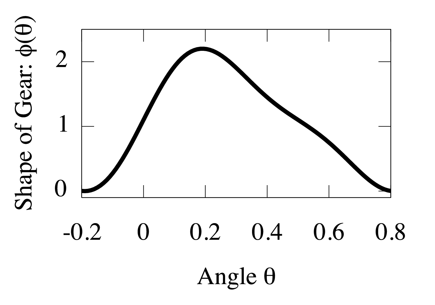
We performed numerical simulations of the FS ratchet with U⁡(θ,x)=k​x2/2+λ​[x−ϕ⁡(θ)]2/2,ϕ⁡(θ)=sin⁡(2​π​θ)+0.25​sin⁡(4​π​θ)+1.1U(\theta,x)=kx^{2}/2+\lambda[x-\phi(\theta)]^{2}/2,\phi(\theta)=\sin(2\pi\theta)+0.25\sin(4\pi\theta)+1.1, Γ=5.0,γ=0.05,k=1.0,Th=1.1,Tc=0.9\Gamma=5.0,\gamma=0.05,k=1.0,T_{h}=1.1,T_{c}=0.9. In this setting, Lx=Tc/λL_{x}=\sqrt{T_{c}/\lambda} and the shortest time scale included in τ\tau is Γ/Th=4.5\Gamma/T_{h}=4.5. To obtain the limit of Model-3, we introduced λ0\lambda_{0} as λ=λ0/m\lambda=\lambda_{0}/m and changed mm and λ0\lambda_{0} as parameters to control the separation of time scales. The limit of λ0→∞\lambda_{0}\to\infty corresponds to the tight confinement of the pawl to the ratchet, ε≃γ/λ​τΠ→0\varepsilon\simeq\gamma/\lambda\tau_{\Pi}\to 0. The limit of m→0m\to 0 realizes the overdamped limit, τΠ/τ=m​Th/Γ2→0\tau_{\Pi}/\tau=mT_{h}/\Gamma^{2}\to 0, while keeping the ratio of γ/λ\gamma/\lambda to τΠ\tau_{\Pi} proportional to λ0\lambda_{0}. The functional form of ϕ⁡(θ)\phi(\theta) is shown in Figure 3. By choosing ϕ⁡(θ)\phi(\theta) to be asymmetric, Ueff​(θ)U_{\mathrm{eff}}(\theta) and Teff​(θ)T_{\mathrm{eff}}(\theta) obtained from Eqs. (5,7) become out of phase as shown in Figure 4.
Refer to caption
Figure 3: The functional forms of ϕ⁡(θ)=sin⁡(2​π​θ)+0.25​sin⁡(4​π​θ)+1.1\phi(\theta)=\sin(2\pi\theta)+0.25\sin(4\pi\theta)+1.1 we used for the numerical simulation.
Refer to caption G ( θ )
Figure 4: The functional forms of Ueff​(θ),𝒢​(θ)U_{\mathrm{eff}}(\theta),\mathcal{G}(\theta) and Teff​(θ)T_{\mathrm{eff}}(\theta) [Eqs. (5-7)] which follow from the setup in the numerical simulation, U⁡(θ,x)=k​x2/2+λ​[x−ϕ⁡(θ)]2/2,ϕ⁡(θ)=sin⁡(2​π​θ)+0.25​sin⁡(4​π​θ)+1.1U(\theta,x)=kx^{2}/2+\lambda[x-\phi(\theta)]^{2}/2,\phi(\theta)=\sin(2\pi\theta)+0.25\sin(4\pi\theta)+1.1. The temperature difference between the positions of positive and negative potential slopes causes a net flow.

The other details of the numerical simulations are illustrated in Appendix D.

V.1 Entropy Production Rates

Numerical results of the steady-state entropy production rates are plotted in Figure 5.

Refer to caption ⟨ σ 1 ⟩ R.h.s of Eq. () τ Π / γ λ ⟨ σ 1 ⟩ ⟨ σ 2 ⟩ R.h.s. of Eq. () = ϵ - 1 / Γ T h τ Π ∼ ϵ - 1
Figure 5: Steady state entropy production rates. Filled circles and squares are the numerical results. Solid lines are obtained through Eqs. (25,26), respectively. The dashed line ∼ϵ−1\sim\epsilon^{-1} shows the asymptotic dependence of ⟨σ1⟩\langle\sigma_{1}\rangle on ϵ\epsilon.

In the tightly confined regime ε−1≃τΠ/(γ/λ)≳40\varepsilon^{-1}\simeq\tau_{\Pi}/(\gamma/\lambda)\gtrsim 40, ⟨σ1⟩\langle\sigma_{1}\rangle converges to the right hand side of Eq. (25).

Next, fixing the parameter at the tightly confined regime, τΠ/(γ/λ)=80\tau_{\Pi}/(\gamma/\lambda)=80, we see the convergence of ⟨σ2⟩\langle\sigma_{2}\rangle to the right hand side of Eq. (26), in the overdamped limit ϵ:=τΠ/τ→0\epsilon:=\tau_{\Pi}/\tau\to 0. Furthermore, we see that ⟨σ1⟩\langle\sigma_{1}\rangle diverges with ϵ−1\epsilon^{-1}, consistent with Eq. (27).

V.2 Thermodynamic Efficiencies

To demonstrate the impact of hidden entropy production, we calculated the thermodynamic efficiencies defined at Models-1, 2 and 3. In Model-1, the thermodynamic efficiency is η1:=1−⟨Qc⟩/⟨Q1h⟩\eta_{1}:=1-\langle Q^{c}\rangle/\langle Q^{h}_{1}\rangle. For Models-2 and 3, however, the definition of the efficiency is not trivial, since there is only a single heat bath with non-uniform continuous temperature. We here adopt a generalized definition of efficiency [46]. The average heat flux conditional on the effective temperature TT is introduced by

⟨Q2,3​(T)⟩:=⟨Q2,3​δ​(Teff​(θ)−T)⟩.\displaystyle\langle Q_{2,3}(T)\rangle:=\langle Q_{2,3}\delta(T_{\mathrm{eff}}(\theta)-T)\rangle. (54)

The averaged heat release and absorption rates are then defined as

⟨Q2,3r​e​l⟩=∫d​T​⟨Q2,3​(T)⟩​Θ​(⟨Q2,3​(T)⟩),⟨Q2,3a​b​s⟩=−∫dT⟨Q2,3(T)⟩Θ(−⟨Q2,3(T)⟩),\displaystyle\begin{split}\left\langle Q_{2,3}^{rel}\right\rangle&=\int dT\langle Q_{2,3}(T)\rangle\Theta(\langle Q_{2,3}(T)\rangle),\\ \left\langle Q_{2,3}^{abs}\right\rangle&=-\int dT\langle Q_{2,3}(T)\rangle\Theta(-\langle Q_{2,3}(T)\rangle),\end{split} (55)

where Θ\Theta represents the Heaviside step function. The generalized efficiencies η2\eta_{2} and η3\eta_{3} are

η2,3=1−⟨Q2,3r​e​l⟩⟨Q2,3a​b​s⟩.\displaystyle\eta_{2,3}=1-\frac{\left\langle Q_{2,3}^{rel}\right\rangle}{\left\langle Q_{2,3}^{abs}\right\rangle}. (56)

For Model-3, this definition agrees with the efficiency introduced as Eq. (49) for the special case of sawtooth potential in the discrete stepping limit.

The dependence of the efficiencies on ff and ϵ\epsilon are shown in Figure 6.

Refer to captionRefer to caption ϵ 0.20 0.10 0.04 0.02 0.01 η 1 η 2
Figure 6: Thermodynamic efficiencies as functions of the external torque ff. In the left figure, η1\eta_{1} and η2\eta_{2} are parametrized by the separation of time scales ϵ\epsilon. Smaller symbols correspond to cases of smaller epsilon. In the right figure, η3\eta_{3} is plotted. The efficiencies are normalized by Carnot efficiency ηC=1−Tc/Th\eta_{C}=1-T_{c}/T_{h}.

The behavior of η1\eta_{1} and η2\eta_{2} are different from that of η3\eta_{3} at ϵ→0\epsilon\to 0. First, η1\eta_{1} approaches to 00 regardless of ff, since it follows from Eq. (11) that the steady-state power, W˙=−f​⟨θ˙⟩\dot{W}=-f\langle\dot{\theta}\rangle, is of O⁡(τ−1)O(\tau^{-1}), while the heat flows at the rate with O⁡(τΠ−1)O(\tau_{\Pi}^{-1}). Second, η2\eta_{2} does not converge to zero (Figure 6). The finite efficiency means that ⟨Q2a​b​s⟩\langle Q_{2}^{abs}\rangle is of the same order as W˙=O⁡(τ−1)\dot{W}=O(\tau^{-1}). Here, ⟨Q2a​b​s⟩\langle Q_{2}^{abs}\rangle fails to capture the heat flow of O⁡(τΠ−1)O(\tau_{\Pi}^{-1}) which contributes to the hidden entropy production ⟨σ1⟩−⟨σ2⟩\langle\sigma_{1}\rangle-\langle\sigma_{2}\rangle. Nevertheless, η2\eta_{2} vanishes at the stalled state, since ⟨Q2a​b​s⟩\langle Q_{2}^{abs}\rangle is kept finite while W˙→0\dot{W}\to 0. Third, η3\eta_{3} monotonically increases and reaches the maximal value at the stalled state. This corresponds to the seemingly reversible situation, ⟨σ3⟩=0\langle\sigma_{3}\rangle=0. However, η3\eta_{3} does not reach Carnot efficiency ηC\eta_{C}, because 1.0<Teff​(θ)<1.11.0<T_{\mathrm{eff}}(\theta)<1.1 as is shown in Figure 4, which implies η3<1−1.0/1.1<ηC\eta_{3}<1-1.0/1.1<\eta_{C}. In Figure 7, we show the ϵ\epsilon-dependence of maximal efficiency, ηim​a​x:=maxf⁡ηi\eta^{max}_{i}:=\max_{f}\eta_{i}, obtained from the fitting of torque-efficiency curves.

Refer to caption ϵ
Figure 7: Maximal efficiency, ηim​a​x=maxf⁡ηi\eta^{max}_{i}=\max_{f}\eta_{i}. Maximal value of η1\eta_{1} and η2\eta_{2} obtained from the fitting of Figure 6 by parabolic functions are plotted against ϵ\epsilon. Solid lines Aexp(−ϵ/ϵ0)+CA\exp(-\epsilon/\epsilon_{0})+C are also plotted as guide for eyes, where A,ϵ0A,\epsilon_{0} and CC are fitting parameters. The efficiencies are normalized by Carnot efficiency of Model-0, ηC=1−Tc/Th\eta_{C}=1-T_{c}/T_{h}.

This result indicates that, in the limit of ϵ→0\epsilon\to 0, η1\eta_{1} vanishes irrespective of ff, and η2\eta_{2} converges to a certain torque-dependent curve.

These results highlight the effects of coarse-graining on the qualitative behaviors of thermodynamic efficiency; one may assume a significantly higher efficiency of an engine by neglecting the dissipative contributions of the fast variables.

VI Recovery of Entropy Production based on Decomposition of Coarse-grained Langevin Dynamics

The exact expression of the entropy production rate in the tightly confined limit [Eq. (25)] inspires us to consider if it is possible to reconstruct the thermodynamic irreversibility defined at the fine-grained description from the observation at the coarse-grained scale. In a system where the time scales of variables are well-separated, it is challenging to probe the dynamics of the fast variable, meaning that the hidden entropy production and the real thermodynamic efficiency are almost impossible to measure [24]. Although there is no general workaround to the problem of inaccessible fast variables, we here describe a way to evaluate ⟨σ1⟩\langle\sigma_{1}\rangle from Model-2 of the FS ratchet.

This is achieved by considering the dynamics as a mixture of two Langevin dynamics with different temperatures and frictions corresponding to the two heat baths (Figure 1d), instead of a single set of effective temperature and friction [Eqs. (6,7)]. The dynamics we consider consists of two Langevin equations,

θ˙=Πm,Π˙=−Γb​(θ)m​Π−∂Ueff​(θ)∂θ+f+2​Γb​(θ)​Tb​ξ,\displaystyle\begin{split}\dot{\theta}=&\frac{\Pi}{m},\\ \dot{\Pi}=&-\frac{\Gamma_{b}(\theta)}{m}\Pi-\frac{\partial U_{\mathrm{eff}}(\theta)}{{\partial\theta}}+f+\sqrt{2\Gamma_{b}(\theta)T_{b}}\xi,\end{split} (57)

and stochastic switching of an auxiliary variable b=h,cb=h,c, which controls which heat bath [(Γh,Th)(\Gamma_{h},T_{h}) or (Γc,Tc)(\Gamma_{c},T_{c})] the Langevin dynamics should be governed by. The stochastic process of θ,Π\theta,\Pi and bb is described by the master equation:

∂P⁡(θ,Π,b)∂t=−∂∂θ​(Πm​P​(θ,Π,b))\displaystyle\frac{\partial P(\theta,\Pi,b)}{{\partial t}}=-\frac{\partial}{{\partial\theta}}\left(\frac{\Pi}{m}P(\theta,\Pi,b)\right)
−∂∂Π​[(−Γb​(θ)m​Π−∂Ueff​(θ)∂θ+f−Γb​(θ)​Tb​∂∂Π)​P​(θ,Π,b)]\displaystyle-\frac{\partial}{{\partial\Pi}}\left[\left(-\frac{\Gamma_{b}(\theta)}{m}\Pi-\frac{\partial U_{\mathrm{eff}}(\theta)}{{\partial\theta}}+f-\Gamma_{b}(\theta)T_{b}\frac{\partial}{{\partial\Pi}}\right)P(\theta,\Pi,b)\right]
−Λ​P​(θ,Π,b)+Λ​P​(θ,Π,b′),\displaystyle-\Lambda P(\theta,\Pi,b)+\Lambda P(\theta,\Pi,b^{\prime}), (Model-6)

where, b′=c,hb^{\prime}=c,h for b=h,cb=h,c, P⁡(θ,Π,b)P(\theta,\Pi,b) is the joint probability density of θ,Π\theta,\Pi and bb, and Λ\Lambda is the rate of stochastic switching of the heat baths. According to the singular perturbation theory, in the limit where Λ−1\Lambda^{-1} is separated from τΠ\tau_{\Pi} and τ\tau, Model-6 will give effective dynamics that follows

θ˙=ΠmΠ˙=−Γh​(θ)+Γc​(θ)2​m​Π−∂Ueff​(θ)∂θ+f+[Γh​(θ)​Th+Γc​(θ)​Tc]​Ξ.\displaystyle\begin{split}\dot{\theta}=&\frac{\Pi}{m}\\ \dot{\Pi}=&-\frac{\Gamma_{h}(\theta)+\Gamma_{c}(\theta)}{2m}\Pi-\frac{\partial U_{\mathrm{eff}}(\theta)}{{\partial\theta}}+f\\ &+\sqrt{[\Gamma_{h}(\theta)T_{h}+\Gamma_{c}(\theta)T_{c}]}\Xi.\end{split} (58)

Therefore, by setting Γh​(θ)=2​Γ\Gamma_{h}(\theta)=2\Gamma and Γc​(θ)=2​γ​ϕ′​(θ)2\Gamma_{c}(\theta)=2\gamma\phi^{\prime}(\theta)^{2}, Eq. (58) will reproduce the dynamics of Model-2.

The entropy production of Model-6 is

σ6=−1Tb(Π˙+∂Ueff​(θ)∂θ−f)∘Πm+1t′−tlnΛbt→bt′​(θ)Λbt′→bt​(θ).\displaystyle\sigma_{6}=-\frac{1}{T_{b}}\left(\dot{\Pi}+\frac{\partial U_{\mathrm{eff}}(\theta)}{{\partial\theta}}-f\right)\circ\frac{\Pi}{m}+\frac{1}{t^{\prime}-t}\ln\frac{\Lambda_{b_{t}\to b_{t^{\prime}}}(\theta)}{\Lambda_{b_{t^{\prime}}\to b_{t}}(\theta)}. (59)

In the limit of fast switching, ⟨σ6⟩\langle\sigma_{6}\rangle converges to the weighted average of the contributions from the two dynamics,

⟨σ6⟩→{Λ​τΠ,Λ​τ}→∞\displaystyle\langle\sigma_{6}\rangle\xrightarrow{\{\Lambda\tau_{\Pi},\Lambda\tau\}\to\infty} 12⟨−1Th(Π˙+∂Ueff​(θ)∂θ−f)∘Πm⟩h\displaystyle\frac{1}{2}\left\langle-\frac{1}{T_{h}}\left(\dot{\Pi}+\frac{\partial U_{\mathrm{eff}}(\theta)}{{\partial\theta}}-f\right)\circ\frac{\Pi}{m}\right\rangle_{h}
+12⟨−1Tc(Π˙+∂Ueff​(θ)∂θ−f)∘Πm⟩c,\displaystyle+\frac{1}{2}\left\langle-\frac{1}{T_{c}}\left(\dot{\Pi}+\frac{\partial U_{\mathrm{eff}}(\theta)}{{\partial\theta}}-f\right)\circ\frac{\Pi}{m}\right\rangle_{c}, (60)

where the subscripts h,ch,c indicate which Langevin dynamics are used to calculate the ensemble average. By comparing Eq. (25) [or Eq. (118)] with Eq. (60), we obtain

lim{Λ​τΠ,Λ​τ}→∞⟨σ6⟩=limε→0⟨σ1⟩.\displaystyle\lim_{\{\Lambda\tau_{\Pi},\Lambda\tau\}\to\infty}\langle\sigma_{6}\rangle=\lim_{\varepsilon\to 0}\langle\sigma_{1}\rangle. (61)

The details of the derivation of Eq. (58) and Eq. (61) are given in Appendix F.

Equation (61) is useful when we know the original temperatures of the heat baths but can only observe the dynamics at the coarse-grained scale. Since 𝒢⁡(θ)\mathcal{G}(\theta) and Teff​(θ)T_{\rm eff}(\theta) can be measured at the coarse-grained scale, we may solve Eqs. (6, 7) using ThT_{h} and TcT_{c} to obtain Γb​(θ)\Gamma_{b}(\theta) in such a situation, which allows the evaluation of ⟨σ6⟩\langle\sigma_{6}\rangle. We note that the decomposition of Model-2 into dynamics involving ThT_{h} and TcT_{c} is not unique if we are allowed to use general θ\theta-dependent switching rates. Nevertheless, we may show that Eq. (61) always holds as far as Model-2 is obtained in the fast switching limit (see Appendix F). The formulation of entropy production based on the decomposition of the stochastic transition has been previously discussed [28, 43, 18]. The approach here is a natural extension of these strategies to the case of a heat engine described by continuous variables.

VII Discussion and Conclusion

We derived the coarse-grained descriptions of the FS ratchet starting from Model-0 along the routes shown in Figure 2. We obtained the exact expressions for the entropy production in each model and clarified the existence of the hidden entropy productions, which correspond to the differences in the entropy production between the different descriptions. The impact of the hidden entropy production on the thermodynamic efficiency was investigated numerically, to track how the efficiency of Models-2 and 3 significantly overestimate the true thermodynamic efficiency of Model-0. Additionally, we proposed a way to reconstruct the entropy production for Model-0 from the coarse-grained scale by introducing pseudo-dynamics described by Model-6.

In this paper, some of the coarse-grained descriptions obtained in this work have been studied previously, e.g. BL motor (Models-2 and 3), two-variable overdamped model (Model-4), single-variable model (Model-3), and the discrete stepping model (Sec. IV-IV.4). This means that the previous works [26, 44, 37, 30, 47, 29, 48, 49, 50, 51, 52, 53, 54, 55] based on phenomenological arguments were correct when taking appropriate timescale separation limits. However, the thermodynamic efficiency of the FS ratchet based on these models have been controversial and often misleading. For instance, the analysis regarding the FS ratchet as the BL motor suffers (Models-2 and 3) from the hidden entropy production. This means that the thermodynamic efficiency of the BL motor is always an overestimation. Similarly, the efficiencies of single-variable models such as Models-3 or 5 [29, 48, 49, 50, 51, 52, 53, 54, 55] are also overestimations. Although a part of studies [29, 48, 49, 50, 51, 52] take into consideration the dissipation corresponding the hidden entropy production, it has been overlooked that hidden dissipations can exist for every coarse-graining step. A two-variable overdamped model used in [37] corresponds Model-4. Since the coarse-graining from Model-0 to Model-4 does not accompany the hidden entropy production, the efficiency obtained in Model-4 appropriately reflects the efficiency of the FS ratchet. In [37], it is concluded that the efficiency is lower than Carnot efficiency. In summary, previous works stating that the FS ratchet can attain Carnot efficiency have all used a coarse-grained version of the model and neglected the hidden dissipation. When appropriate models and dissipations are taken to account, Carnot efficiency cannot be obtained.

The problem of hidden entropy production is inevitable when analysing the thermodynamic aspect of nonequilibrium system, since any model is considered to be constructed phenomenologically. In this sense, Model-6 points at a promising solution for the hidden entropy production. It enables us to evaluate the true entropy production without knowing the true fine-grained description (Model-0). Therefore, it is important to develop such a framework, which may extract thermodynamic properties from the coarse-grained descriptions.

Acknowledgements.
We thank E. Muneyuki, S. Wang, Y. Murashita and M. Itami for fruitful comments. This work is supported by the Grant-in-Aids for JSPS Fellow No. 24-3258 (YN), No. 24-8031 and No. 28-908 (KK), the Grant-in-Aid For Young Scientists (B) No. 17K14373 (YN), and JSPS KAKENHI Grants No. 15K05196 and No. 25103002 (NN).

Appendix A Derivation of Coarse-grained Dynamics

A.1 Derivation of Model-2

In this subsection, we describe the details of the derivation of Model-2. Our goal here is to obtain the time evolution equation of the joint probability density P⁡(θ,Π)P(\theta,\Pi) from Eq. (2). We evaluate the last term of the right hand side of Eq. (3) in the limit of ε:=τx/τΠ→0\varepsilon:=\tau_{x}/\tau_{\Pi}\to 0. The heart of the singular perturbation theory is to decompose the time-dependence of P⁡(θ,Π,x)P(\theta,\Pi,x) into the explicit part and the implicit part through P⁡(θ,Π)P(\theta,\Pi). In the limit of ε→0\varepsilon\to 0, the explicit part decays quickly and the right hand side of Eq. (3) essentially turns into a functional of P⁡(θ,Π)P(\theta,\Pi).

A singular perturbation problem is mapped to an ordinary perturbation theory by introducing MM which describes P⁡(θ,Π,x)P(\theta,\Pi,x) and Ω\Omega which describes the dynamics of P⁡(θ,Π)P(\theta,\Pi). For this purpose, we first switch the variables from (t,x)(t,x) to the dimensionless time and distance

𝒯\displaystyle\mathcal{T} :=tτx,\displaystyle:=\frac{t}{\tau_{x}}, s\displaystyle s :=x−ϕ⁡(θ)Lx,\displaystyle:=\frac{x-\phi(\theta)}{L_{x}}, (62)

and rewrite Eq. (2) as

τx−1​∂P⁡(θ,Π,s)∂𝒯=(ℒθ+ℒΠ)​P​(θ,Π,s)\displaystyle\tau_{x}^{-1}\frac{\partial P(\theta,\Pi,s)}{{\partial\mathcal{T}}}=(\mathcal{L}^{\theta}+\mathcal{L}^{\Pi})P(\theta,\Pi,s)
+τx−1/2[γTcϕ′(θ)(∂∂sΠm−∂∂Π∂U~I​(s)∂s)P(θ,Π,s)]\displaystyle+\tau_{x}^{-1/2}\left[\sqrt{\frac{\gamma}{T_{c}}}\phi^{\prime}(\theta)\left(\frac{\partial}{{\partial s}}\frac{\Pi}{m}-\frac{\partial}{{\partial\Pi}}\frac{\partial\tilde{U}_{I}(s)}{{\partial s}}\right)P(\theta,\Pi,s)\right]
−τx−1​∂∂s​[−1Tc​∂U~I​(s)∂s​P​(θ,Π,s)−∂P⁡(θ,Π,s)∂s]\displaystyle-\tau_{x}^{-1}\frac{\partial}{{\partial s}}\left[-\frac{1}{T_{c}}\frac{\partial\tilde{U}_{I}(s)}{{\partial s}}P(\theta,\Pi,s)-\frac{\partial P(\theta,\Pi,s)}{{\partial s}}\right]
−τx−1/2∂∂s[−Tcγ(U0′​(ϕ⁡(θ))Tc+O(|U0′′|​Lx|U0′|))P(θ,Π,s)],\displaystyle-\tau_{x}^{-1/2}\frac{\partial}{{\partial s}}\left[-\sqrt{\frac{T_{c}}{\gamma}}\left(\frac{U_{0}^{\prime}(\phi(\theta))}{T_{c}}+O\left(\frac{|U_{0}^{\prime\prime}|L_{x}}{|U_{0}^{\prime}|}\right)\right)P(\theta,\Pi,s)\right], (63)

where

ℒθ:=\displaystyle\mathcal{L}^{\theta}:= −∂∂θ​Πm,\displaystyle-\frac{\partial}{{\partial\theta}}\frac{\Pi}{m}, ℒΠ:=\displaystyle\mathcal{L}^{\Pi}:= −∂∂Π​[(−Γm​Π+f)−Γ​Th​∂∂Π].\displaystyle-\frac{\partial}{{\partial\Pi}}\left[\left(-\frac{\Gamma}{m}\Pi+f\right)-\Gamma T_{h}\frac{\partial}{{\partial\Pi}}\right]. (64)

In terms of τx,τΠ\tau_{x},\tau_{\Pi} and τ\tau, we may estimate the order of the terms in the right hand side of Eq. (63) as O(τ−1)+O(τΠ−1),O(τx−1/2τΠ−1/2),O(τx−1)O(\tau^{-1})+O(\tau_{\Pi}^{-1}),O(\tau_{x}^{-1/2}\tau_{\Pi}^{-1/2}),O(\tau_{x}^{-1}) and O(τx−1/2τ−1/2)O(\tau_{x}^{-1/2}\tau^{-1/2}), respectively. In addition, O⁡(|U0′′|​Lx/|U0′|)=O⁡[(τx/τ)1/2]O(|U^{\prime\prime}_{0}|L_{x}/|U^{\prime}_{0}|)=O[(\tau_{x}/\tau)^{1/2}]. Based on this order estimation, we may consider ε\varepsilon as the small parameter which controls the perturbative analysis.

The explicit and implicit dependence of P⁡(θ,Π,s)P(\theta,\Pi,s) on 𝒯\mathcal{T} is implemented by describing P⁡(θ,Π,s)P(\theta,\Pi,s) as output of a 𝒯\mathcal{T}-dependent operator, MM, that acts on P⁡(θ,Π)P(\theta,\Pi):

P⁡(θ,Π,s)=M⁡[P⁡(θ′,Π′);𝒯]​(θ,Π,s),\displaystyle P(\theta,\Pi,s)=M[P(\theta^{\prime},\Pi^{\prime});\mathcal{T}](\theta,\Pi,s), (65)

where θ′\theta^{\prime} and Π′\Pi^{\prime} are dummy variables placed only to indicate that MM depends on the joint probability density of θ\theta and Π\Pi. Furthermore, we represent the time-evolution of P⁡(θ,Π)P(\theta,\Pi) by a 𝒯\mathcal{T}-dependent operator Ω\Omega that acts on P⁡(θ,Π)P(\theta,\Pi):

∂P⁡(θ,Π)∂𝒯=Ω⁡[P⁡(θ′,Π′);𝒯]​(θ,Π):=τx​(ℒθ+ℒΠ)​P​(θ,Π)\displaystyle\frac{\partial P(\theta,\Pi)}{{\partial\mathcal{T}}}=\Omega[P(\theta^{\prime},\Pi^{\prime});\mathcal{T}](\theta,\Pi):=\tau_{x}(\mathcal{L}^{\theta}+\mathcal{L}^{\Pi})P(\theta,\Pi)
−∂∂Π​[τx1/2​γTc​ϕ′​(θ)​∫d​s​∂U~I​(s)∂s​M​[P⁡(θ′,Π′);𝒯]​(θ,Π,s)],\displaystyle-\frac{\partial}{{\partial\Pi}}\left[\tau_{x}^{1/2}\sqrt{\frac{\gamma}{T_{c}}}\phi^{\prime}(\theta)\int ds\frac{\partial\tilde{U}_{I}(s)}{{\partial s}}M[P(\theta^{\prime},\Pi^{\prime});\mathcal{T}](\theta,\Pi,s)\right], (66)

which is obtained by integrating Eq. (63) with respect to ss. Since MM depends on 𝒯\mathcal{T} explicitly and implicitly [through P⁡(θ,Π)P(\theta,\Pi)], the substitution of MM into the left hand side of Eq. (63) gives

[l.h.s. of Eq. (63)]=∂M⁡[P⁡(θ′,Π′);𝒯]​(θ,Π,s)∂𝒯\displaystyle[\mbox{l.h.s. of Eq.~(\ref{e:scaled})}]=\frac{\partial M[P(\theta^{\prime},\Pi^{\prime});\mathcal{T}](\theta,\Pi,s)}{{\partial\mathcal{T}}}
+∫dθ′′dΠ′′∂P⁡(θ′′,Π′′)∂𝒯δ​M​[P⁡(θ′′,Π′′);𝒯]​(θ,Π,s)δ​P​(θ′′,Π′′)\displaystyle\hskip 43.05542pt+\int d\theta^{\prime\prime}d\Pi^{\prime\prime}\frac{\partial P(\theta^{\prime\prime},\Pi^{\prime\prime})}{{\partial\mathcal{T}}}\frac{\delta M[P(\theta^{\prime\prime},\Pi^{\prime\prime});\mathcal{T}](\theta,\Pi,s)}{\delta P(\theta^{\prime\prime},\Pi^{\prime\prime})}
=∂M⁡[P⁡(θ′,Π′);𝒯]​(θ,Π,s)∂𝒯\displaystyle=\frac{\partial M[P(\theta^{\prime},\Pi^{\prime});\mathcal{T}](\theta,\Pi,s)}{{\partial\mathcal{T}}}
+∫dθ′′dΠ′′Ω[P(θ′,Π′);𝒯](θ′′,Π′′)δ​M​[P⁡(θ′′,Π′′);𝒯]​(θ,Π,s)δ​P​(θ′′,Π′′),\displaystyle+\int d\theta^{\prime\prime}d\Pi^{\prime\prime}\Omega[P(\theta^{\prime},\Pi^{\prime});\mathcal{T}](\theta^{\prime\prime},\Pi^{\prime\prime})\frac{\delta M[P(\theta^{\prime\prime},\Pi^{\prime\prime});\mathcal{T}](\theta,\Pi,s)}{\delta P(\theta^{\prime\prime},\Pi^{\prime\prime})}, (67)

according to the chain rule. Applying Eq. (65) also in the right hand side of Eq. (63), we obtain

∂M⁡[P⁡(θ′,Π′);𝒯]​(θ,Π,s)∂𝒯\displaystyle\frac{\partial M[P(\theta^{\prime},\Pi^{\prime});\mathcal{T}](\theta,\Pi,s)}{{\partial\mathcal{T}}}
+∫dθ′′dΠ′′Ω[P(θ′,Π′);𝒯](θ′′,Π′′)δ​M​[P⁡(θ′′,Π′′);𝒯]​(θ,Π,s)δ​P​(θ′′,Π′′)\displaystyle+\int d\theta^{\prime\prime}d\Pi^{\prime\prime}\Omega[P(\theta^{\prime},\Pi^{\prime});\mathcal{T}](\theta^{\prime\prime},\Pi^{\prime\prime})\frac{\delta M[P(\theta^{\prime\prime},\Pi^{\prime\prime});\mathcal{T}](\theta,\Pi,s)}{\delta P(\theta^{\prime\prime},\Pi^{\prime\prime})}
=τx​(ℒθ+ℒΠ)​M​[P⁡(θ′,Π′);𝒯]​(θ,Π,s)\displaystyle=\tau_{x}(\mathcal{L}^{\theta}+\mathcal{L}^{\Pi})M[P(\theta^{\prime},\Pi^{\prime});\mathcal{T}](\theta,\Pi,s)
+τx1/2​γTc​ϕ′​(θ)​(∂∂s​Πm−∂∂Π​∂U~I​(s)∂s)​M​[P⁡(θ′,Π′);𝒯]​(θ,Π,s)\displaystyle+\tau_{x}^{1/2}\sqrt{\frac{\gamma}{T_{c}}}\phi^{\prime}(\theta)\left(\frac{\partial}{{\partial s}}\frac{\Pi}{m}-\frac{\partial}{{\partial\Pi}}\frac{\partial\tilde{U}_{I}(s)}{{\partial s}}\right)M[P(\theta^{\prime},\Pi^{\prime});\mathcal{T}](\theta,\Pi,s)
−∂∂s​[−1Tc​∂U~I​(s)∂s−∂∂s]​M​[P⁡(θ′,Π′);𝒯]​(θ,Π,s)\displaystyle-\frac{\partial}{{\partial s}}\left[-\frac{1}{T_{c}}\frac{\partial\tilde{U}_{I}(s)}{{\partial s}}-\frac{\partial}{{\partial s}}\right]M[P(\theta^{\prime},\Pi^{\prime});\mathcal{T}](\theta,\Pi,s)
−∂∂s​[−τx1/2​Tcγ​(U0′​(ϕ⁡(θ))Tc+O⁡(ε1/2))​M​[P⁡(θ′,Π′);𝒯]​(θ,Π,s)].\displaystyle-\frac{\partial}{{\partial s}}\left[-\tau_{x}^{1/2}\sqrt{\frac{T_{c}}{\gamma}}\left(\frac{U_{0}^{\prime}(\phi(\theta))}{T_{c}}+O\left(\varepsilon^{1/2}\right)\right)M[P(\theta^{\prime},\Pi^{\prime});\mathcal{T}](\theta,\Pi,s)\right]. (68)

The remaining task is to apply the standard procedure of perturbation theory. We expand MM and Ω\Omega into series of ε1/2\varepsilon^{1/2}:

M⁡[P⁡(θ′,Π′);𝒯]​(θ,Π,s)\displaystyle M[P(\theta^{\prime},\Pi^{\prime});\mathcal{T}](\theta,\Pi,s) =∑n=0εn/2​M(n)​[P⁡(θ′,Π′);𝒯]​(θ,Π,s),\displaystyle=\sum_{n=0}\varepsilon^{n/2}M^{(n)}[P(\theta^{\prime},\Pi^{\prime});\mathcal{T}](\theta,\Pi,s), (69)
Ω⁡[P⁡(θ′,Π′);𝒯]​(θ,Π)\displaystyle\Omega[P(\theta^{\prime},\Pi^{\prime});\mathcal{T}](\theta,\Pi) =∑n=0ε(n+1)/2​Ω(n)​[P⁡(θ′,Π′);𝒯]​(θ,Π).\displaystyle=\sum_{n=0}\varepsilon^{(n+1)/2}\Omega^{(n)}[P(\theta^{\prime},\Pi^{\prime});\mathcal{T}](\theta,\Pi). (70)

Here, the difference in the lowest order for MM and Ω\Omega is due to Eqs. (66). The leading order of Eq. (68) gives

∂M(0)​[P⁡(θ′,Π′);𝒯]​(θ,Π,s)∂𝒯\displaystyle\frac{\partial M^{(0)}[P(\theta^{\prime},\Pi^{\prime});\mathcal{T}](\theta,\Pi,s)}{{\partial\mathcal{T}}}
=−∂∂s​[−1Tc​∂U~I​(s)∂s−∂∂s]​M(0)​[P⁡(θ′,Π′);𝒯]​(θ,Π,s),\displaystyle=-\frac{\partial}{{\partial s}}\left[-\frac{1}{T_{c}}\frac{\partial\tilde{U}_{I}(s)}{{\partial s}}-\frac{\partial}{{\partial s}}\right]M^{(0)}[P(\theta^{\prime},\Pi^{\prime});\mathcal{T}](\theta,\Pi,s), (71)

from which we obtain

M(0)​[P⁡(θ′,Π′);𝒯]​(θ,Π,s)=P⁡(θ,Π)​exp(−U~I(s)/Tc)Z+…,\displaystyle{M^{(0)}[P(\theta^{\prime},\Pi^{\prime});\mathcal{T}](\theta,\Pi,s)}=P(\theta,\Pi)\frac{\exp\left(-{\tilde{U}_{I}(s)}/{T_{c}}\right)}{Z}+..., (72)

where Z=∫dsexp(−U~I(s)/Tc)Z=\int ds\exp\left(-\tilde{U}_{I}(s)/T_{c}\right). The additional terms … depend on 𝒯\mathcal{T} explicitly, and can be neglected since they decay exponentially with the time scale of O⁡(τx)O(\tau_{x}). Under this assumption of the time scale, Ω(0)​[P⁡(θ′,Π′);𝒯]​(θ,Π)\Omega^{(0)}[P(\theta^{\prime},\Pi^{\prime});\mathcal{T}](\theta,\Pi) vanishes, since the last term in the right hand side of Eq. (66) is zero in the leading order. The sub-leading order of Eq. (68) is

∂M(1)​[P⁡(θ′,Π′);𝒯]​(θ,Π,s)∂𝒯\displaystyle\frac{\partial M^{(1)}[P(\theta^{\prime},\Pi^{\prime});\mathcal{T}](\theta,\Pi,s)}{{\partial\mathcal{T}}}
=(τxε)1/2​γTc​ϕ′​(θ)​(∂∂s​Πm−∂∂Π​∂U~I​(s)∂s)​M(0)​[P⁡(θ′,Π′);𝒯]​(θ,Π,s)\displaystyle=\left(\frac{\tau_{x}}{\varepsilon}\right)^{1/2}\sqrt{\frac{\gamma}{T_{c}}}\phi^{\prime}(\theta)\left(\frac{\partial}{{\partial s}}\frac{\Pi}{m}-\frac{\partial}{{\partial\Pi}}\frac{\partial\tilde{U}_{I}(s)}{{\partial s}}\right)M^{(0)}[P(\theta^{\prime},\Pi^{\prime});\mathcal{T}](\theta,\Pi,s)
−∂∂s[(−1Tc∂U~I​(s)∂s−∂∂s)M(1)[P(θ′,Π′);𝒯](θ,Π,s)\displaystyle-\frac{\partial}{{\partial s}}\left[\left(-\frac{1}{T_{c}}\frac{\partial\tilde{U}_{I}(s)}{{\partial s}}-\frac{\partial}{{\partial s}}\right)M^{(1)}[P(\theta^{\prime},\Pi^{\prime});\mathcal{T}](\theta,\Pi,s)\right.
−(τxε)1/2TcγU0′​(ϕ⁡(θ))TcM(0)[P(θ′,Π′);𝒯](θ,Π,s)],\displaystyle\phantom{-\frac{1}{\gamma}\frac{\partial}{{\partial 2}}\Bigg(}\left.-\left(\frac{\tau_{x}}{\varepsilon}\right)^{1/2}\sqrt{\frac{T_{c}}{\gamma}}\frac{U_{0}^{\prime}(\phi(\theta))}{T_{c}}M^{(0)}[P(\theta^{\prime},\Pi^{\prime});\mathcal{T}](\theta,\Pi,s)\right], (73)

which has a particular solution

M(1)​[P⁡(θ′,Π′);𝒯]​(θ,Π,s)\displaystyle{M^{(1)}[P(\theta^{\prime},\Pi^{\prime});\mathcal{T}](\theta,\Pi,s)}
∝s​exp(−U~I(s)/Tc)Z​[−γ​ϕ′​(θ)​(Πm+Tc​∂∂Π)−U0′​(ϕ⁡(θ))]​P​(θ,Π)\displaystyle\propto s\frac{\exp\left(-{\tilde{U}_{I}(s)}/{T_{c}}\right)}{Z}\left[-\gamma\phi^{\prime}(\theta)\left(\frac{\Pi}{m}+T_{c}\frac{\partial}{{\partial\Pi}}\right)-{U_{0}^{\prime}(\phi(\theta))}\right]P(\theta,\Pi)
+[exponentially decaying terms].\displaystyle+[\mbox{exponentially decaying terms}]. (74)

By substituting Eq. (74) into Eq. (66),

Ω(1)​[P⁡(θ′,Π′);𝒯]\displaystyle\Omega^{(1)}[P(\theta^{\prime},\Pi^{\prime});\mathcal{T}]
=−τxε​{∂∂θ​[Πm​P​(θ,Π)]+∂∂Π​[(−Γm​Π+f)−Γ​Th​∂∂Π]​P​(θ,Π)}\displaystyle=-\frac{\tau_{x}}{\varepsilon}\left\{\frac{\partial}{{\partial\theta}}\left[\frac{\Pi}{m}P(\theta,\Pi)\right]+\frac{\partial}{{\partial\Pi}}\left[\left(-\frac{\Gamma}{m}\Pi+f\right)-\Gamma T_{h}\frac{\partial}{{\partial\Pi}}\right]P(\theta,\Pi)\right\}
−∂∂Π​[(τxε)1/2​γTc​ϕ′​(θ)​∫d​s​∂U~I​(s)∂s​M(1)​[P⁡(θ′,Π′);𝒯]​(θ,Π,s)]\displaystyle-\frac{\partial}{{\partial\Pi}}\left[\left(\frac{\tau_{x}}{\varepsilon}\right)^{1/2}\sqrt{\frac{\gamma}{T_{c}}}\phi^{\prime}(\theta)\int ds\frac{\partial\tilde{U}_{I}(s)}{{\partial s}}M^{(1)}[P(\theta^{\prime},\Pi^{\prime});\mathcal{T}](\theta,\Pi,s)\right]
=\displaystyle= −τxε{∂∂θ[ΠmP(θ,Π)]+∂∂Π[(−ΓmΠ+f)−ΓTh∂∂Π]P(θ,Π)\displaystyle-\frac{\tau_{x}}{\varepsilon}\Bigg\{\frac{\partial}{{\partial\theta}}\left[\frac{\Pi}{m}P(\theta,\Pi)\right]+\frac{\partial}{{\partial\Pi}}\left[\left(-\frac{\Gamma}{m}\Pi+f\right)-\Gamma T_{h}\frac{\partial}{{\partial\Pi}}\right]P(\theta,\Pi)
+∂∂Π[−γϕ′(θ)2(Πm+Tc∂∂Π)−ϕ′(θ)U0′(ϕ(θ))]P(θ,Π)}.\displaystyle+\frac{\partial}{{\partial\Pi}}\left[-\gamma\phi^{\prime}(\theta)^{2}\left(\frac{\Pi}{m}+T_{c}\frac{\partial}{{\partial\Pi}}\right)-\phi^{\prime}(\theta){U^{\prime}_{0}(\phi(\theta))}\right]P(\theta,\Pi)\Bigg\}. (75)

The Kramers equation [Eq. (4)] immediately follows from the relation, ∂P⁡(θ,Π)/∂𝒯=Ω⁡[P⁡(θ′,Π′);𝒯]\partial P(\theta,\Pi)/\partial\mathcal{T}=\Omega[P(\theta^{\prime},\Pi^{\prime});\mathcal{T}] with Eqs. (5, 6, 7).

A.2 Quick Derivation of Model-2

In the procedure of temporal coarse-graining, we first formally solve the equation of motion of eliminated variable, xx, [Eq. (8)] as

xt=\displaystyle x_{t}= 1γ​∫−∞td​t′​e−k+λγ​(t−t′)​[λ​ϕ​(θt′)+2​γ​Tc​ζ~t′]\displaystyle\frac{1}{\gamma}\int_{-\infty}^{t}dt^{\prime}e^{-\frac{k+\lambda}{\gamma}(t-t^{\prime})}\left[\lambda\phi(\theta_{t^{\prime}})+\sqrt{2\gamma T_{c}}\tilde{\zeta}_{t^{\prime}}\right]
=\displaystyle= λk+λ​ϕ​(θ)−γ​λ(k+λ)2​ϕ′​(θt)​Πtm​[1+o⁡(ε)]\displaystyle\frac{\lambda}{k+\lambda}\phi(\theta)-\frac{\gamma\lambda}{(k+\lambda)^{2}}\phi^{\prime}(\theta_{t})\frac{\Pi_{t}}{m}\left[1+o\left(\varepsilon\right)\right]
+2​γ​Tcγ∫−∞tdt′e−k+λγ​(t−t′)ζ~t′.\displaystyle+\frac{\sqrt{2\gamma T_{c}}}{\gamma}\int_{-\infty}^{t}dt^{\prime}e^{-\frac{k+\lambda}{\gamma}(t-t^{\prime})}\tilde{\zeta}_{t^{\prime}}. (76)

Here, we performed integration by part twice. The substitution of Eq. (76) into the equation of motion of Π\Pi gives Eq (9). As done in [41], the underdamped Langevin equation is obtained by integrating Eq. (9) over t∈[t0,t0+Δ​t]t\in[t_{0},t_{0}+\Delta t], using the identity

∫t0t0+Δ​td​t​∫−∞td​t′=\displaystyle\int_{t_{0}}^{{t_{0}}+\Delta t}dt\int_{-\infty}^{t}dt^{\prime}= ∫−∞t0d​t′​∫t0t0+Δ​t𝑑t+∫t0t0+Δ​td​t′​∫t′t0+Δ​t𝑑t.\displaystyle\int_{-\infty}^{t_{0}}dt^{\prime}\int_{t_{0}}^{{t_{0}}+\Delta t}dt+\int_{t_{0}}^{{t_{0}}+\Delta t}dt^{\prime}\int_{t^{\prime}}^{{t_{0}}+\Delta t}dt. (77)

By neglecting the O⁡(2​γ​Tc​λk+λ​∫−∞t0d​t′​e−k+λγ​(t0−t′)​ζ~t′)O\left(\sqrt{2\gamma T_{c}}\frac{\lambda}{k+\lambda}\int_{-\infty}^{t_{0}}dt^{\prime}e^{-\frac{k+\lambda}{\gamma}({t_{0}}-t^{\prime})}\tilde{\zeta}_{t^{\prime}}\right) term, we obtain

Πt0+Δ​t−Πt0Δ​t=\displaystyle\frac{\Pi_{{t_{0}}+\Delta t}-\Pi_{t_{0}}}{\Delta t}= −Γ+γ​λ2(k+λ)2​ϕ′​(θt)2m​Π+f−k​λk+λ​ϕ′​(θ)​ϕ​(θ)\displaystyle-\frac{\Gamma+\frac{\gamma\lambda^{2}}{(k+\lambda)^{2}}\phi^{\prime}(\theta_{t})^{2}}{m}\Pi+f-\frac{k\lambda}{k+\lambda}\phi^{\prime}(\theta)\phi(\theta)
+2​Γ​Th​ξt+2​γ​ϕ′​(θt)2​Tc​λk+λ​1Δ​t​∫t0t0+Δ​td​t′​ζ~t′.\displaystyle+\sqrt{2\Gamma T_{h}}\xi_{t}+\sqrt{2\gamma\phi^{\prime}(\theta_{t})^{2}T_{c}}\frac{\lambda}{k+\lambda}\frac{1}{\Delta t}\int_{t_{0}}^{{t_{0}}+\Delta t}dt^{\prime}\tilde{\zeta}_{t^{\prime}}. (78)

Since m/k\sqrt{m/k} should be included in the set of slow time scales, k/λ=O⁡(τx/τ)=O⁡(ε)k/\lambda=O(\tau_{x}/\tau)=O(\varepsilon). Therefore, Eq. (78) results in Model-2 in the limit of ε→0\varepsilon\to 0.

A.3 Derivation of Model-3

The coarse-graining from Model-2 to Model-3 can also be formulated through the framework of Appendix A-A.1. By introducing the dimensionless time and momentum

𝒯~\displaystyle\tilde{\mathcal{T}} =tτΠ,\displaystyle=\frac{t}{\tau_{\Pi}}, ϖ\displaystyle\varpi =Πm​T0,\displaystyle=\frac{\Pi}{\sqrt{mT_{0}}}, (79)

where T0T_{0} is the reference point of temperature, the Kramers equation [Eq. (4)] corresponding to Model-2 may be rewritten as

Γm​∂P⁡(θ,ϖ)∂𝒯~=\displaystyle\frac{\Gamma}{m}\frac{\partial P(\theta,\varpi)}{{\partial\tilde{\mathcal{T}}}}= −∂∂θ​(T0m​ϖ​P​(θ,ϖ))\displaystyle-\frac{\partial}{{\partial\theta}}\left(\sqrt{\frac{T_{0}}{m}}\varpi P(\theta,\varpi)\right)
−∂∂ϖ[(−1m​T0∂Ueff​(θ)∂θ+1m​T0f)P(θ,ϖ)\displaystyle-\frac{\partial}{{\partial\varpi}}\left[\left(-\frac{1}{\sqrt{mT_{0}}}\frac{\partial U_{\mathrm{eff}}(\theta)}{{\partial\theta}}+\frac{1}{\sqrt{mT_{0}}}f\right)P(\theta,\varpi)\right.
−Γm𝒢⁡(θ)Γ(ϖP(θ,ϖ)−Teff​(θ)T0∂P⁡(θ,ϖ)∂ϖ)].\displaystyle\left.-\frac{\Gamma}{m}\frac{\mathcal{G}(\theta)}{\Gamma}\left(\varpi P(\theta,\varpi)-\frac{T_{\mathrm{eff}}(\theta)}{T_{0}}\frac{\partial P(\theta,\varpi)}{{\partial\varpi}}\right)\right]. (80)

The first, second and third lines are O(τ−1),O(τ−1/2τΠ−1/2)O(\tau^{-1}),O(\tau^{-1/2}\tau_{\Pi}^{-1/2}) and O⁡(τΠ−1)O(\tau_{\Pi}^{-1}), respectively. Following the procedure in Appendix A-A.1, we define

M~​[P⁡(θ′);𝒯~]​(θ,ϖ)\displaystyle\tilde{M}[P(\theta^{\prime});\tilde{\mathcal{T}}](\theta,\varpi) :=P⁡(θ,ϖ)\displaystyle:=P(\theta,\varpi) (81)
Ω~​[P⁡(θ′);𝒯~]​(θ)\displaystyle\tilde{\Omega}[P(\theta^{\prime});\tilde{\mathcal{T}}](\theta) :=−τΠ∫dϖ∂∂θ(T0mϖM~[P(θ′);𝒯~](θ,ϖ))\displaystyle:=-\tau_{\Pi}\int d\varpi\frac{\partial}{{\partial\theta}}\left(\sqrt{\frac{T_{0}}{m}}\varpi\tilde{M}[P(\theta^{\prime});\tilde{\mathcal{T}}](\theta,\varpi)\right) (82)
=∫d​ϖ​∂P⁡(θ,ϖ)∂𝒯~=∂P⁡(θ)∂𝒯~,\displaystyle=\int d\varpi\frac{\partial P(\theta,\varpi)}{{\partial\tilde{\mathcal{T}}}}=\frac{\partial P(\theta)}{{\partial\tilde{\mathcal{T}}}}, (83)

where P⁡(θ)=∫d​ϖ​P​(θ,ϖ)P(\theta)=\int d\varpi P(\theta,\varpi). In the standard perturbation theory of Eq. (80) expressed in terms of M~\tilde{M} and Ω~\tilde{\Omega} with a small parameter ϵ:=τΠ/τ\epsilon:=\tau_{\Pi}/\tau, the leading order gives,

∂M~(0)​[P⁡(θ′);𝒯~]​(θ,ϖ)∂𝒯~\displaystyle\frac{\partial\tilde{M}^{(0)}[P(\theta^{\prime});\tilde{\mathcal{T}}](\theta,\varpi)}{{\partial\tilde{\mathcal{T}}}}
=−∂∂ϖ​[−𝒢⁡(θ)Γ​ϖ−𝒢⁡(θ)Γ​Teff​(θ)T0​∂∂ϖ]​M~(0)​[P⁡(θ′);𝒯~]​(θ,ϖ),\displaystyle=-\frac{\partial}{{\partial\varpi}}\left[-\frac{\mathcal{G}(\theta)}{\Gamma}\varpi-\frac{\mathcal{G}(\theta)}{\Gamma}\frac{T_{\mathrm{eff}}(\theta)}{T_{0}}\frac{\partial}{{\partial\varpi}}\right]{\tilde{M}^{(0)}[P(\theta^{\prime});\tilde{\mathcal{T}}](\theta,\varpi)}, (84)

which has a solution

M~(0)​[P⁡(θ′);𝒯~]​(θ,ϖ)=\displaystyle\tilde{M}^{(0)}[P(\theta^{\prime});\tilde{\mathcal{T}}](\theta,\varpi)= P⁡(θ)​exp⁡(−T0​ϖ22​T​(θ))2​π​T​(θ)\displaystyle P(\theta)\frac{\exp\left(-\frac{T_{0}\varpi^{2}}{2T(\theta)}\right)}{\sqrt{2\pi T(\theta)}}
+[exponentially decaying terms].\displaystyle+[\mbox{exponentially decaying terms}]. (85)

Since Ω~(0)​[P⁡(θ′);𝒯~]​(θ)\tilde{\Omega}^{(0)}[P(\theta^{\prime});\tilde{\mathcal{T}}](\theta) vanishes again, we proceed to the sub-leading order of Eq. (80),

∂M~(1)​[P⁡(θ′);𝒯~]​(θ,ϖ)∂𝒯~=−τ​∂∂θ​(T0m​ϖ​M~(0)​[P⁡(θ′);𝒯~]​(θ,ϖ))\displaystyle\frac{\partial\tilde{M}^{(1)}[P(\theta^{\prime});\tilde{\mathcal{T}}](\theta,\varpi)}{{\partial\tilde{\mathcal{T}}}}=-\tau\frac{\partial}{{\partial\theta}}\left(\sqrt{\frac{T_{0}}{m}}{\varpi}\tilde{M}^{(0)}[P(\theta^{\prime});\tilde{\mathcal{T}}](\theta,\varpi)\right)
−τ​∂∂ϖ​[1m​T0​(−∂Ueff​(θ)∂θ+f)​M~(0)​[P⁡(θ′);𝒯~]​(θ,ϖ)]\displaystyle-\tau\frac{\partial}{{\partial\varpi}}\left[\frac{1}{\sqrt{mT_{0}}}\left(-\frac{\partial U_{\mathrm{eff}}(\theta)}{{\partial\theta}}+f\right)\tilde{M}^{(0)}[P(\theta^{\prime});\tilde{\mathcal{T}}](\theta,\varpi)\right]
−∂∂ϖ​[−𝒢⁡(θ)Γ​ϖ−𝒢⁡(θ)Γ​Teff​(θ)T0​∂∂ϖ]​M~(1)​[P⁡(θ′);𝒯~]​(θ,ϖ),\displaystyle-\frac{\partial}{{\partial\varpi}}\left[-\frac{\mathcal{G}(\theta)}{\Gamma}\varpi-\frac{\mathcal{G}(\theta)}{\Gamma}\frac{T_{\mathrm{eff}}(\theta)}{T_{0}}\frac{\partial}{{\partial\varpi}}\right]{\tilde{M}^{(1)}[P(\theta^{\prime});\tilde{\mathcal{T}}](\theta,\varpi)}, (86)

which has a particular solution

M~(1)[P(θ′);𝒯~](θ,ϖ)={−∂P⁡(θ)∂θ\displaystyle\tilde{M}^{(1)}[P(\theta^{\prime});\tilde{\mathcal{T}}](\theta,\varpi)=\left\{-\frac{\partial P(\theta)}{{\partial\theta}}\right.
−[(T0​ϖ26​Teff​(θ)+12)Teff′​(θ)Teff​(θ)+1Teff​(θ)(∂Ueff​(θ)∂θ−f)]P(θ)}\displaystyle\left.-\left[\left(\frac{T_{0}\varpi^{2}}{6T_{\mathrm{eff}}(\theta)}+\frac{1}{2}\right)\frac{T_{\mathrm{eff}}^{\prime}(\theta)}{T_{\mathrm{eff}}(\theta)}+\frac{1}{T_{\mathrm{eff}}(\theta)}\left(\frac{\partial U_{\mathrm{eff}}(\theta)}{{\partial\theta}}-f\right)\right]P(\theta)\right\}
⋅τ​T0m​Γ𝒢⁡(θ)​ϖ​exp(−T0ϖ2/2T(θ))2​π​T​(θ)\displaystyle\cdot\tau\sqrt{\frac{T_{0}}{m}}\frac{\Gamma}{\mathcal{G}(\theta)}\varpi\frac{\exp\left(-{T_{0}\varpi^{2}}/{2T(\theta)}\right)}{\sqrt{2\pi T(\theta)}}
+[exponentially decaying terms].\displaystyle+[\mbox{exponentially decaying terms}]. (87)

By substituting Eq. (87) into Eq. (82),

Ω~(1)[P(θ′);𝒯~](θ):=−τ∫dϖ∂∂θ(T0mϖM~(1)[P(θ′);𝒯~](θ,ϖ))\displaystyle\tilde{\Omega}^{(1)}[P(\theta^{\prime});\tilde{\mathcal{T}}](\theta):=-\tau\int d\varpi\frac{\partial}{{\partial\theta}}\left(\sqrt{\frac{T_{0}}{m}}\varpi\tilde{M}^{(1)}[P(\theta^{\prime});\tilde{\mathcal{T}}](\theta,\varpi)\right)
=\displaystyle= −τ​∂∂θ​{1𝒢⁡(θ)​[(−∂Ueff​(θ)∂θ+f)​P​(θ)−∂∂θ​[Teff​(θ)​P​(θ)]]}.\displaystyle-\tau\frac{\partial}{{\partial\theta}}\left\{\frac{1}{\mathcal{G}(\theta)}\left[\left(-\frac{\partial U_{\mathrm{eff}}(\theta)}{{\partial\theta}}+f\right)P(\theta)-\frac{\partial}{{\partial\theta}}[T_{\textrm{eff}}(\theta){P(\theta)}]\right]\right\}. (88)

We finally reach

∂P⁡(θ)∂t\displaystyle\frac{\partial P(\theta)}{{\partial t}} (89)
=\displaystyle= −∂∂θ​{1𝒢⁡(θ)​[(−∂Ueff​(θ)∂θ+f)​P​(θ)−∂∂θ​[Teff​(θ)​P​(θ)]]}.\displaystyle-\frac{\partial}{{\partial\theta}}\left\{\frac{1}{\mathcal{G}(\theta)}\left[\left(-\frac{\partial U_{\mathrm{eff}}(\theta)}{{\partial\theta}}+f\right)P(\theta)-\frac{\partial}{{\partial\theta}}[{T_{\textrm{eff}}(\theta)P(\theta)}]\right]\right\}.

In order to obtain the overdamped Langevin equation corresponding to Eq. (89), we first recall that [56]

X˙=A⁡(X)+C⁡(X)∘Ξ~,\displaystyle\dot{X}=A(X)+C(X)\circ\tilde{\Xi}, (90)

can be mapped to an additive Langevin equation

X¯˙=A¯​(X¯)+Ξ~,\displaystyle\dot{\bar{X}}=\bar{A}(\bar{X})+\tilde{\Xi}, (91)

where Ξ~\tilde{\Xi} is a white Gaussian noise with zero mean and unit variance, and X¯=∫X𝑑X/C⁡(X),A¯​(X¯)=A⁡(X)/C⁡(X)\bar{X}=\int^{X}dX/C(X),\bar{A}(\bar{X})=A(X)/C(X). Since Eq. (91) has a corrsponding Fokker-Planck equation

∂P⁡(X¯)∂t=−∂∂X¯​(A¯​(X¯)​P​(X¯)−12​∂P⁡(X¯)∂X¯),\displaystyle\frac{\partial P(\bar{X})}{{\partial t}}=-\frac{\partial}{{\partial\bar{X}}}\left(\bar{A}(\bar{X})P(\bar{X})-\frac{1}{2}\frac{\partial P(\bar{X})}{{\partial\bar{X}}}\right), (92)

we obtain the Fokker-Planck equation for P⁡(X)P(X) through variable transformation [note that P⁡(X¯)=P⁡(X)​C​(X)P(\bar{X})=P(X)C(X)]:

∂P⁡(X)∂t=−∂∂X​(A⁡(X)​P​(X)−C⁡(X)2​∂∂X​[C⁡(X)​P​(X)]).\displaystyle\frac{\partial P(X)}{{\partial t}}=-\frac{\partial}{{\partial X}}\left(A(X)P(X)-\frac{C(X)}{2}\frac{\partial}{{\partial X}}[C(X)P(X)]\right). (93)

Therefore, by rewriting Eq. (89) in the form of Eq. (93), the Langevin equation corresponding to Eq. (89) is obtained as

θ˙=\displaystyle\dot{\theta}= 1𝒢⁡(θ)​(−∂Ueff​(θ)∂θ+f)−12​𝒢​(θ)2​∂∂θ​[𝒢⁡(θ)​Teff​(θ)]\displaystyle\frac{1}{\mathcal{G}(\theta)}\left(-\frac{\partial U_{\mathrm{eff}}(\theta)}{{\partial\theta}}+f\right)-\frac{1}{2\mathcal{G}(\theta)^{2}}\frac{\partial}{{\partial\theta}}\left[{\mathcal{G}(\theta)}{T_{\mathrm{eff}}(\theta)}\right]
+2​Teff​(θ)𝒢⁡(θ)∘Ξ~.\displaystyle+\sqrt{2\frac{T_{\mathrm{eff}}(\theta)}{\mathcal{G}(\theta)}}\circ\tilde{\Xi}. (94)

By changing the product, we have

θ˙=1𝒢⁡(θ)​(−∂Ueff​(θ)∂θ+f)+2𝒢⁡(θ)⊙Teff​(θ)⋅Ξ~.\displaystyle\dot{\theta}=\frac{1}{\mathcal{G}(\theta)}\left(-\frac{\partial U_{\mathrm{eff}}(\theta)}{{\partial\theta}}+f\right)+\sqrt{\frac{2}{\mathcal{G}(\theta)}}\odot\sqrt{{T_{\mathrm{eff}}(\theta)}}\cdot\tilde{\Xi}. (95)

Multiplying 𝒢⁡(θ)\mathcal{G}(\theta) in the sense of anti-Itô to both sides

𝒢⁡(θ)⊙θ˙=(−∂Ueff​(θ)∂θ+f)+2​𝒢​(θ)⊙Teff​(θ)⋅Ξ~.\displaystyle{\mathcal{G}(\theta)}\odot\dot{\theta}=\left(-\frac{\partial U_{\mathrm{eff}}(\theta)}{{\partial\theta}}+f\right)+\sqrt{2{\mathcal{G}(\theta)}}\odot\sqrt{{T_{\mathrm{eff}}(\theta)}}\cdot\tilde{\Xi}. (96)

A.4 Derivation of Model-5

We start by rescaling the variables in Eq. (14) by Eq. (62).

τx−1​∂P⁡(θ,s)∂𝒯=−∂∂θ​[fΓ​P​(θ,s)−ThΓ​∂∂θ​P​(θ,s)]\displaystyle\tau_{x}^{-1}\frac{\partial P(\theta,s)}{{\partial\mathcal{T}}}=-\frac{\partial}{{\partial\theta}}\left[\frac{f}{\Gamma}P(\theta,s)-\frac{T_{h}}{\Gamma}\frac{\partial}{{\partial\theta}}{P(\theta,s)}\right]
+τx−1/2γTc∂∂s[ϕ′(θ)(fΓP(θ,s)−ThΓ∂∂θP(θ,s))]\displaystyle+\tau_{x}^{-1/2}\sqrt{\frac{\gamma}{T_{c}}}\frac{\partial}{{\partial s}}\left[\phi^{\prime}(\theta)\left(\frac{f}{\Gamma}P(\theta,s)-\frac{T_{h}}{\Gamma}\frac{\partial}{{\partial\theta}}{P(\theta,s)}\right)\right]
−τx−1/2γTc∂∂θ[ϕ′​(θ)Γ∂UI​(s)∂sP(θ,s)+ϕ′​(θ)ΓTh∂∂sP(θ,s)]\displaystyle-\tau_{x}^{-1/2}\sqrt{\frac{\gamma}{T_{c}}}\frac{\partial}{{\partial\theta}}\left[\frac{\phi^{\prime}(\theta)}{\Gamma}\frac{\partial U_{I}(s)}{{\partial s}}P(\theta,s)+\frac{\phi^{\prime}(\theta)}{\Gamma}T_{h}\frac{\partial}{{\partial s}}{P(\theta,s)}\right]
+τx−1/2γTc∂∂s{1γ[∂U0​(ϕ​(θ))∂ϕ⁡(θ)+O(τxτ)]P(θ,s)}\displaystyle+\tau_{x}^{-1/2}\sqrt{\frac{\gamma}{T_{c}}}\frac{\partial}{{\partial s}}\left\{\frac{1}{\gamma}\left[\frac{\partial U_{0}(\phi(\theta))}{{\partial\phi(\theta)}}+O\left(\frac{\tau_{x}}{\tau}\right)\right]P(\theta,s)\right\}
−τx−11Γ​Tc∂∂s[−(Γ+γϕ′(θ)2)∂UI​(s)∂sP(θ,s)\displaystyle-\tau_{x}^{-1}\frac{1}{\Gamma T_{c}}\frac{\partial}{{\partial s}}\left[-\left({\Gamma+\gamma\phi^{\prime}(\theta)^{2}}\right)\frac{\partial U_{I}(s)}{{\partial s}}P(\theta,s)\right.
−(ΓTc+γϕ′(θ)2Th)∂∂sP(θ,s)].\displaystyle\phantom{-\tau_{x}^{-1}\frac{1}{\Gamma T_{c}}\frac{\partial}{{\partial s}}\Bigg[}\left.-\left({\Gamma T_{c}+\gamma\phi^{\prime}(\theta)^{2}T_{h}}\right)\frac{\partial}{{\partial s}}{P(\theta,s)}\right]. (97)

The first line of Eq. (97) is O⁡(τ−1)O(\tau^{-1}), the last two lines are O⁡(τx−1)O(\tau_{x}^{-1}), and the remaining terms are O(τ−1/2τx−1/2)O(\tau^{-1/2}\tau_{x}^{-1/2}), respectively. Again, following the procedure in Appendix A-A.1, we define

M^​[P⁡(θ′);𝒯]​(θ,s):=P⁡(θ,s)\displaystyle\hat{M}[P(\theta^{\prime});\mathcal{T}](\theta,s):=P(\theta,s) (98)
Ω^​[P⁡(θ′);𝒯]​(θ):=−τx​∂∂θ​[fΓ​P​(θ)−ThΓ​∂∂θ​P​(θ)]\displaystyle\hat{\Omega}[P(\theta^{\prime});\mathcal{T}](\theta):=-\tau_{x}\frac{\partial}{{\partial\theta}}\left[\frac{f}{\Gamma}P(\theta)-\frac{T_{h}}{\Gamma}\frac{\partial}{{\partial\theta}}{P(\theta)}\right]
−τx1/2​γTc​∂∂θ​[∫d​s​ϕ′​(θ)Γ​∂UI​(s)∂s​M^​[P⁡(θ′);𝒯]​(θ,s)].\displaystyle-\tau_{x}^{1/2}\sqrt{\frac{\gamma}{T_{c}}}\frac{\partial}{{\partial\theta}}\left[\int ds\frac{\phi^{\prime}(\theta)}{\Gamma}\frac{\partial U_{I}(s)}{{\partial s}}\hat{M}[P(\theta^{\prime});\mathcal{T}](\theta,s)\right]. (99)

Now, we apply the standard perturbation theory to Eq. (97) expressed in terms of M^\hat{M} and Ω^\hat{\Omega}, with a small parameter ε′=τx/τ\varepsilon^{\prime}=\tau_{x}/\tau. The leading order of Eq. (97) gives

∂M^(0)∂𝒯=\displaystyle\frac{\partial\hat{M}^{(0)}}{{\partial\mathcal{T}}}= −1Γ​Tc​∂∂s​[−𝒢⁡(θ)​∂UI​(s)∂s​M^(0)−𝒢⁡(θ)​Ts​(θ)​∂∂s​M^(0)],\displaystyle-\frac{1}{\Gamma T_{c}}\frac{\partial}{{\partial s}}\left[-\mathcal{G}(\theta)\frac{\partial U_{I}(s)}{{\partial s}}\hat{M}^{(0)}-\mathcal{G}(\theta)T_{s}(\theta)\frac{\partial}{{\partial s}}{\hat{M}^{(0)}}\right], (100)

where

Ts​(θ)=Th​γ​ϕ′​(θ)2+Tc​ΓΓ+γ​ϕ′​(θ)2.\displaystyle T_{s}(\theta)=\frac{T_{h}\gamma\phi^{\prime}(\theta)^{2}+T_{c}\Gamma}{\Gamma+\gamma\phi^{\prime}(\theta)^{2}}. (101)

We obtain

M^(0)=P⁡(θ)​exp⁡(−UI​(s)Ts​(θ))z⁡(θ)+[exponentially decaying terms],\displaystyle\hat{M}^{(0)}=P(\theta)\frac{\exp{\left(-\frac{U_{I}(s)}{T_{s}(\theta)}\right)}}{z(\theta)}+[\mbox{exponentially decaying terms}], (102)

with

z⁡(θ)=∫d​s​exp⁡(−UI​(s)Ts​(θ)).\displaystyle z(\theta)=\int ds\,{\exp{\left(-\frac{U_{I}(s)}{T_{s}(\theta)}\right)}}. (103)

In the time scale of τ\tau, the O⁡(ε′1/2)O(\varepsilon^{\prime 1/2}) term of Ω^\hat{\Omega} vanishes. The sub-leading order of Eq. (97) becomes

∂M^(1)∂𝒯=τ−1/2γTc∂∂s[ϕ′(θ)(fΓM^(0)−ThΓ∂∂θM^(0))]\displaystyle\frac{\partial\hat{M}^{(1)}}{{\partial\mathcal{T}}}=\tau^{-1/2}\sqrt{\frac{\gamma}{T_{c}}}\frac{\partial}{{\partial s}}\left[\phi^{\prime}(\theta)\left(\frac{f}{\Gamma}\hat{M}^{(0)}-\frac{T_{h}}{\Gamma}\frac{\partial}{{\partial\theta}}{\hat{M}^{(0)}}\right)\right]
−τ−1/2γTc∂∂θ[ϕ′​(θ)Γ∂UI​(s)∂sM^(0)+ϕ′​(θ)ΓTh∂∂sM^(0)]\displaystyle-\tau^{-1/2}\sqrt{\frac{\gamma}{T_{c}}}\frac{\partial}{{\partial\theta}}\left[\frac{\phi^{\prime}(\theta)}{\Gamma}\frac{\partial U_{I}(s)}{{\partial s}}\hat{M}^{(0)}+\frac{\phi^{\prime}(\theta)}{\Gamma}T_{h}\frac{\partial}{{\partial s}}{\hat{M}^{(0)}}\right]
+τ−1/2γTc∂∂s[1γ∂U0​(ϕ​(θ))∂ϕ⁡(θ)M^(0)]\displaystyle+\tau^{-1/2}\sqrt{\frac{\gamma}{T_{c}}}\frac{\partial}{{\partial s}}\left[\frac{1}{\gamma}\frac{\partial U_{0}(\phi(\theta))}{{\partial\phi(\theta)}}{\hat{M}^{(0)}}\right]
−1Γ​Tc​∂∂s​[−𝒢⁡(θ)​∂UI​(s)∂s​M^(1)−𝒢⁡(θ)​Ts​(θ)​∂∂s​M^(1)],\displaystyle-\frac{1}{\Gamma T_{c}}\frac{\partial}{{\partial s}}\left[-\mathcal{G}(\theta)\frac{\partial U_{I}(s)}{{\partial s}}\hat{M}^{(1)}-\mathcal{G}(\theta)T_{s}(\theta)\frac{\partial}{{\partial s}}{\hat{M}^{(1)}}\right], (104)

which gives

M^(1)∝\displaystyle\hat{M}^{(1)}\propto −s​M^(0)𝒢⁡(θ)​Ts​(θ){−∂∂θ[ϕ′​(θ)Γ(Th−Ts(θ))]+fΓϕ′(θ)\displaystyle\frac{-s\hat{M}^{(0)}}{\mathcal{G}(\theta)T_{s}(\theta)}\left\{-\frac{\partial}{{\partial\theta}}\left[\frac{\phi^{\prime}(\theta)}{\Gamma}(T_{h}-T_{s}(\theta))\right]+\frac{f}{\Gamma}\phi^{\prime}(\theta)\right.
+1γ∂U0​(ϕ​(θ))∂ϕ⁡(θ)}−ϕ′​(θ)Γ(2Th−Ts(θ))1𝒢⁡(θ)​Ts​(θ)\displaystyle\left.+\frac{1}{\gamma}\frac{\partial U_{0}(\phi(\theta))}{{\partial\phi(\theta)}}\right\}-\frac{\phi^{\prime}(\theta)}{\Gamma}(2T_{h}-T_{s}(\theta))\frac{1}{\mathcal{G}(\theta)T_{s}(\theta)}
[∂∂θ​(s​M^(0))−1Ts​(θ)2​∂Ts​(θ)∂θ​ℐ​(s)​M^(0)]\displaystyle\left[{\frac{\partial}{{\partial\theta}}(s\hat{M}^{(0)})}-\frac{1}{T_{s}(\theta)^{2}}\frac{\partial T_{s}(\theta)}{{\partial\theta}}\mathcal{I}(s)\hat{M}^{(0)}\right]
+[exponentially decaying terms],\displaystyle+[\mbox{exponentially decaying terms}], (105)

where

ℐ⁡(s)=s​UI​(s)−∫sd​s′​UI​(s′).\displaystyle\mathcal{I}(s)=sU_{I}(s)-\int^{s}ds^{\prime}U_{I}(s^{\prime}). (106)

Substitution of Eq. (105) into Eq. (99) results in

Ω^(1)​[P⁡(θ);𝒯]:=−τ​∂∂θ​[fΓ​P​(θ)−ThΓ​∂∂θ​P​(θ)]\displaystyle\hat{\Omega}^{(1)}[P(\theta);\mathcal{T}]:=-\tau\frac{\partial}{{\partial\theta}}\left[\frac{f}{\Gamma}P(\theta)-\frac{T_{h}}{\Gamma}\frac{\partial}{{\partial\theta}}{P(\theta)}\right]
−τ1/2​γTc​∂∂θ​[∫d​s​ϕ′​(θ)Γ​∂UI​(s)∂s​M^(1)​[P⁡(θ′);𝒯]​(θ,s)]\displaystyle-\tau^{1/2}\sqrt{\frac{\gamma}{T_{c}}}\frac{\partial}{{\partial\theta}}\left[\int ds\frac{\phi^{\prime}(\theta)}{\Gamma}\frac{\partial U_{I}(s)}{{\partial s}}\hat{M}^{(1)}[P(\theta^{\prime});\mathcal{T}](\theta,s)\right]
=\displaystyle= −τ∂∂θ[f𝒢⁡(θ)P(θ)+∂∂θ(γ​ϕ′​(θ)22​𝒢​(θ)2)(Th−Tc)P(θ)\displaystyle-\tau\frac{\partial}{{\partial\theta}}\left[\frac{f}{\mathcal{G}(\theta)}P(\theta)+\frac{\partial}{{\partial\theta}}\left(\frac{\gamma\phi^{\prime}(\theta)^{2}}{2\mathcal{G}(\theta)^{2}}\right)(T_{h}-T_{c})P(\theta)\right.
−1𝒢⁡(θ)∂Ueff​(θ)∂θP(θ)−Teff​(θ)𝒢⁡(θ)∂∂θP(θ)],\displaystyle\left.-\frac{1}{\mathcal{G}(\theta)}\frac{\partial U_{\mathrm{eff}}(\theta)}{{\partial\theta}}P(\theta)-\frac{T_{\mathrm{eff}}(\theta)}{\mathcal{G}(\theta)}\frac{\partial}{{\partial\theta}}{P(\theta)}\right], (107)

which gives the Fokker-Planck equation,

∂P⁡(θ)∂t=\displaystyle\frac{\partial P(\theta)}{{\partial t}}= −∂∂θ[−1𝒢⁡(θ)∂ln⁡𝒢⁡(θ)∂θ(Th−Tc)P(θ)\displaystyle-\frac{\partial}{{\partial\theta}}\left[-\frac{1}{\mathcal{G}(\theta)}\frac{\partial\ln\mathcal{G}(\theta)}{{\partial\theta}}(T_{h}-T_{c})P(\theta)\right.
+1𝒢⁡(θ)(f−∂Ueff​(θ)∂θ)P(θ)−1𝒢⁡(θ)∂∂θ(Teff(θ)P(θ))],\displaystyle\left.+\frac{1}{\mathcal{G}(\theta)}\left(f-\frac{\partial U_{\mathrm{eff}}(\theta)}{{\partial\theta}}\right)P(\theta)-\frac{1}{\mathcal{G}(\theta)}\frac{\partial}{{\partial\theta}}{\left({T_{\mathrm{eff}}(\theta)}P(\theta)\right)}\right], (108)

corresponding to Model-5.

Appendix B Asymptotic Behavior of Entropy Production Rates

B.1 Transition Probabilities in Eqs. (15-19)

W1(θt′,Πt′,xt′|θt,Πt,xt)=\displaystyle W_{1}(\theta_{t^{\prime}},\Pi_{t^{\prime}},x_{t^{\prime}}|\theta_{t},\Pi_{t},x_{t})= δ⁡(θt′−θt−Πt+Πt′2​m​(t′−t))​WU​D​(Πt′|Πt;−∂U⁡(θ¯,x¯)∂θ¯+f,Γ,Th)\displaystyle\delta\left(\theta_{t^{\prime}}-\theta_{t}-\frac{\Pi_{t}+\Pi_{t^{\prime}}}{2m}(t^{\prime}-t)\right)W_{UD}\left(\Pi_{t^{\prime}}\bigg|\Pi_{t};-\frac{\partial U(\bar{\theta},\bar{x})}{{\partial\bar{\theta}}}+f,\Gamma,T_{h}\right)
14​π​(t′−t)​Tc/γ​exp⁡(−[γ⁡(xt′−xt)+∂U⁡(θ¯,x¯)/∂x¯​(t′−t)]24​γ​Tc​(t′−t)+∂2U⁡(θ¯,x¯)∂x¯2​(t′−t)2​γ),\displaystyle\frac{1}{\sqrt{4\pi(t^{\prime}-t)T_{c}/\gamma}}\exp\left(-\frac{[\gamma(x_{t^{\prime}}-x_{t})+\partial{U(\bar{\theta},\bar{x})}/\partial{\bar{x}}(t^{\prime}-t)]^{2}}{4\gamma T_{c}(t^{\prime}-t)}+\frac{\partial^{2}U(\bar{\theta},\bar{x})}{{\partial\bar{x}}^{2}}\frac{(t^{\prime}-t)}{2\gamma}\right), (109)
W2(θt′,Πt′|θt,Πt)=\displaystyle W_{2}(\theta_{t^{\prime}},\Pi_{t^{\prime}}|\theta_{t},\Pi_{t})= δ⁡(θt′−θt−Πt+Πt′2​m​(t′−t))​WU​D​(Πt′|Πt;−∂Ueff​(θ¯)∂θ¯+f,𝒢⁡(θ¯),Teff​(θ¯)),\displaystyle\delta\left(\theta_{t^{\prime}}-\theta_{t}-\frac{\Pi_{t}+\Pi_{t^{\prime}}}{2m}(t^{\prime}-t)\right)W_{UD}\left(\Pi_{t^{\prime}}\bigg|\Pi_{t};-\frac{\partial U_{\mathrm{eff}}(\bar{\theta})}{{\partial\bar{\theta}}}+f,\mathcal{G}(\bar{\theta}),T_{\mathrm{eff}}(\bar{\theta})\right), (110)
W3​(θt′|θt)=\displaystyle W_{3}(\theta_{t^{\prime}}|\theta_{t})= 14​π​(t′−t)​Teff​(θ¯)/𝒢⁡(θ¯)​exp⁡(−{𝒢⁡(θ¯)​(θt′−θt)+[∂(Ueff​(θ¯)+Teff​(θ¯))/∂θ¯−f]​(t′−t)}24​𝒢​(θ¯)​Teff​(θ¯)​(t′−t)CLOSE\displaystyle\frac{1}{\sqrt{4\pi(t^{\prime}-t)T_{\mathrm{eff}}(\bar{\theta})/\mathcal{G}(\bar{\theta})}}\exp\left(-\frac{\{\mathcal{G}(\bar{\theta})(\theta_{t^{\prime}}-\theta_{t})+[\partial{(U_{\mathrm{eff}}(\bar{\theta})+T_{\mathrm{eff}}(\bar{\theta}))}/\partial{\bar{\theta}}-f](t^{\prime}-t)\}^{2}}{4\mathcal{G}(\bar{\theta})T_{\mathrm{eff}}(\bar{\theta})(t^{\prime}-t)}\right.
OPEN+12​∂∂θ¯​[1𝒢⁡(θ¯)​(∂Ueff​(θ¯)∂θ¯−f)+Teff​(θ¯)𝒢​(θ¯)2​∂𝒢⁡(θ¯)∂θ¯+12​∂∂θ¯​Teff​(θ¯)𝒢⁡(θ¯)]​(t′−t)),\displaystyle\left.+\frac{1}{2}\frac{\partial}{{\partial\bar{\theta}}}\left[\frac{1}{\mathcal{G}(\bar{\theta})}\left(\frac{\partial U_{\mathrm{eff}}(\bar{\theta})}{{\partial\bar{\theta}}}-f\right)+\frac{T_{\mathrm{eff}}(\bar{\theta})}{\mathcal{G}(\bar{\theta})^{2}}\frac{\partial\mathcal{G}(\bar{\theta})}{{\partial\bar{\theta}}}+\frac{1}{2}\frac{\partial}{{\partial\bar{\theta}}}\frac{T_{\mathrm{eff}}(\bar{\theta})}{\mathcal{G}(\bar{\theta})}\right](t^{\prime}-t)\right), (111)
W4(θt′,xt′|θt,xt)=\displaystyle W_{4}(\theta_{t^{\prime}},x_{t^{\prime}}|\theta_{t},x_{t})= 14​π​(t′−t)​Th/Γ​exp⁡(−[Γ⁡(θt′−θt)+(∂U⁡(θ¯,x¯)/∂θ¯−f)​(t′−t)]24​Γ​Th​(t′−t)+∂2U⁡(θ¯,x¯)∂θ¯2​(t′−t)2​Γ)\displaystyle\frac{1}{\sqrt{4\pi(t^{\prime}-t)T_{h}/\Gamma}}\exp\left(-\frac{[\Gamma(\theta_{t^{\prime}}-\theta_{t})+(\partial{U(\bar{\theta},\bar{x})}/\partial{\bar{\theta}}-f)(t^{\prime}-t)]^{2}}{4\Gamma T_{h}(t^{\prime}-t)}+\frac{\partial^{2}U(\bar{\theta},\bar{x})}{{\partial\bar{\theta}}^{2}}\frac{(t^{\prime}-t)}{2\Gamma}\right)
14​π​(t′−t)​Tc/γ​exp⁡(−[γ⁡(xt′−xt)+∂U⁡(θ¯,x¯)/∂x¯​(t′−t)]24​γ​Tc​(t′−t)+∂2U⁡(θ¯,x¯)∂x¯2​(t′−t)2​γ),\displaystyle\frac{1}{\sqrt{4\pi(t^{\prime}-t)T_{c}/\gamma}}\exp\left(-\frac{[\gamma(x_{t^{\prime}}-x_{t})+\partial{U(\bar{\theta},\bar{x})}/\partial{\bar{x}}(t^{\prime}-t)]^{2}}{4\gamma T_{c}(t^{\prime}-t)}+\frac{\partial^{2}U(\bar{\theta},\bar{x})}{{\partial\bar{x}}^{2}}\frac{(t^{\prime}-t)}{2\gamma}\right), (112)
W5​(θt′|θt)=\displaystyle W_{5}(\theta_{t^{\prime}}|\theta_{t})= 14​π​(t′−t)​Teff​(θ¯)/𝒢⁡(θ¯)​exp⁡(−{𝒢⁡(θ¯)​(θt′−θt)+[∂(Ueff​(θ¯)+Teff​(θ¯))+ln⁡𝒢⁡(θ¯)​(Th−Tc)/∂θ¯−f]​(t′−t)}24​𝒢​(θ¯)​Teff​(θ¯)​(t′−t)CLOSE\displaystyle\frac{1}{\sqrt{4\pi(t^{\prime}-t)T_{\mathrm{eff}}(\bar{\theta})/\mathcal{G}(\bar{\theta})}}\exp\left(-\frac{\{\mathcal{G}(\bar{\theta})(\theta_{t^{\prime}}-\theta_{t})+[\partial{(U_{\mathrm{eff}}(\bar{\theta})+T_{\mathrm{eff}}(\bar{\theta}))+{\ln\mathcal{G}(\bar{\theta})}(T_{h}-T_{c})}/\partial{\bar{\theta}}-f](t^{\prime}-t)\}^{2}}{4\mathcal{G}(\bar{\theta})T_{\mathrm{eff}}(\bar{\theta})(t^{\prime}-t)}\right.
OPEN+12​∂∂θ¯​[1𝒢⁡(θ¯)​(∂Ueff​(θ¯)∂θ¯+∂ln⁡𝒢⁡(θ¯)∂θ¯​(Th−Tc)−f)+Teff​(θ¯)𝒢​(θ¯)2​∂𝒢⁡(θ¯)∂θ¯+12​∂∂θ¯​Teff​(θ¯)𝒢⁡(θ¯)]​(t′−t)),\displaystyle\left.+\frac{1}{2}\frac{\partial}{{\partial\bar{\theta}}}\left[\frac{1}{\mathcal{G}(\bar{\theta})}\left(\frac{\partial U_{\mathrm{eff}}(\bar{\theta})}{{\partial\bar{\theta}}}+\frac{\partial\ln\mathcal{G}(\bar{\theta})}{{\partial\bar{\theta}}}(T_{h}-T_{c})-f\right)+\frac{T_{\mathrm{eff}}(\bar{\theta})}{\mathcal{G}(\bar{\theta})^{2}}\frac{\partial\mathcal{G}(\bar{\theta})}{{\partial\bar{\theta}}}+\frac{1}{2}\frac{\partial}{{\partial\bar{\theta}}}\frac{T_{\mathrm{eff}}(\bar{\theta})}{\mathcal{G}(\bar{\theta})}\right](t^{\prime}-t)\right), (113)

where θ¯=(θt+θt′)/2,x¯=(xt+xt′)/2\bar{\theta}=(\theta_{t}+\theta_{t^{\prime}})/2,\bar{x}=(x_{t}+x_{t^{\prime}})/2, and

WU​D​(Πt′|Πt;F,g,T)=14​π​(t′−t)​T/g​exp⁡(−[Πt′−Πt+(gm​Πt+Πt′2−F)​(t′−t)]24​g​T​(t′−t)),\displaystyle W_{UD}(\Pi_{t^{\prime}}|\Pi_{t};F,g,T)=\frac{1}{\sqrt{4\pi(t^{\prime}-t)T/g}}\exp\left(-\frac{\left[\Pi_{t^{\prime}}-\Pi_{t}+\left(\frac{g}{m}\frac{\Pi_{t}+\Pi_{t^{\prime}}}{2}-F\right)(t^{\prime}-t)\right]^{2}}{4gT(t^{\prime}-t)}\right), (114)

is the transition probability of momentum degree of freedom following the underdamped Langevin equation.

B.2 Derivation of Eq. (25)

Based on the results of Appendix A, we evaluate the ensemble average of the entropy production rate ⟨σ1⟩\langle\sigma_{1}\rangle in the limit of ε→0\varepsilon\to 0. Since ⟨Q1h⟩\langle Q_{1}^{h}\rangle may be rewritten as

⟨Q1h⟩=\displaystyle\langle Q_{1}^{h}\rangle= ⟨−(Π˙+∂U⁡(θ,x)∂θ−f)∘Πm⟩=⟨Γm(Π2m−Th)⟩,\displaystyle\left\langle-\left(\dot{\Pi}+\frac{\partial U(\theta,x)}{{\partial\theta}}-f\right)\circ\frac{\Pi}{m}\right\rangle=\left\langle\frac{\Gamma}{m}\left(\frac{\Pi^{2}}{m}-T_{h}\right)\right\rangle, (115)

we consider the ensemble average of Q1cQ_{1}^{c} with respect to M⁡[P⁡(θ′,Π′);𝒯]​(θ,Π,s)M[P(\theta^{\prime},\Pi^{\prime});\mathcal{T}](\theta,\Pi,s), by replacing xx in Q1cQ_{1}^{c} by ϕ⁡(θ)+Lx​s\phi(\theta)+L_{x}s:

Q1c=\displaystyle Q_{1}^{c}= −∂U⁡(θ,x)∂x∘x˙\displaystyle-\frac{\partial U(\theta,x)}{{\partial x}}\circ\dot{x}
=\displaystyle= −(1Lx∂UI​(s)∂s+∂U0​(ϕ​(θ))∂ϕ⁡(θ)+O(Lx))∘(ϕ′(θ)θ˙+Lxs˙)\displaystyle-\left(\frac{1}{L_{x}}\frac{\partial U_{I}(s)}{{\partial s}}+\frac{\partial U_{0}(\phi(\theta))}{{\partial\phi(\theta)}}+O(L_{x})\right)\circ(\phi^{\prime}(\theta)\dot{\theta}+L_{x}\dot{s})
=\displaystyle= (−1Lx​∂UI​(s)∂s−∂U0​(ϕ​(θ))∂ϕ⁡(θ))​ϕ′​(θ)​Πm−∂UI​(s)∂s∘s˙+O⁡(Lx).\displaystyle\left(-\frac{1}{L_{x}}\frac{\partial U_{I}(s)}{{\partial s}}-\frac{\partial U_{0}(\phi(\theta))}{{\partial\phi(\theta)}}\right)\phi^{\prime}(\theta)\frac{\Pi}{m}-\frac{\partial U_{I}(s)}{{\partial s}}\circ\dot{s}+O(L_{x}). (116)

The ensemble average of the first term of Eq. (116) is [up to O⁡(Lx0)O(L_{x}^{0})],

⟨−ϕ′​(θ)Lx​∂UI​(s)∂s​Πm⟩\displaystyle\left\langle-\frac{\phi^{\prime}(\theta)}{L_{x}}\frac{\partial U_{I}(s)}{{\partial s}}\frac{\Pi}{m}\right\rangle
≃∫dθdΠds[−ϕ′​(θ)LxΠm∂UI​(s)∂sM(0)[P(θ′,Π′);𝒯](θ,Π,s)\displaystyle\simeq\int d\theta d\Pi ds\left[-\frac{\phi^{\prime}(\theta)}{L_{x}}\frac{\Pi}{m}\frac{\partial U_{I}(s)}{{\partial s}}M^{(0)}[P(\theta^{\prime},\Pi^{\prime});\mathcal{T}](\theta,\Pi,s)\right.
−ϕ′(θ)Πm∂UI​(s)∂sγTc​ετxM(1)[P(θ′,Π′);𝒯](θ,Π,s)]\displaystyle\left.-\phi^{\prime}(\theta)\frac{\Pi}{m}\frac{\partial U_{I}(s)}{{\partial s}}\sqrt{\frac{\gamma}{T_{c}}\frac{\varepsilon}{\tau_{x}}}M^{(1)}[P(\theta^{\prime},\Pi^{\prime});\mathcal{T}](\theta,\Pi,s)\right]
=−∫dθdΠdsϕ′(θ)Πm1Tc∂UI​(s)∂ssexp(−UI(s)/Tc)Z\displaystyle=-\int d\theta d\Pi ds\phi^{\prime}(\theta)\frac{\Pi}{m}\frac{1}{T_{c}}\frac{\partial U_{I}(s)}{{\partial s}}s\frac{\exp(-U_{I}(s)/T_{c})}{Z}
[−γ​ϕ′​(θ)​(Πm+Tc​∂∂Π)−U0′​(ϕ⁡(θ))]​P​(θ,Π)\displaystyle\quad\left[-\gamma\phi^{\prime}(\theta)\left(\frac{\Pi}{m}+T_{c}\frac{\partial}{{\partial\Pi}}\right)-U_{0}^{\prime}(\phi(\theta))\right]P(\theta,\Pi)
=⟨γ​ϕ′​(θ)2m​(Π2m−Tc)+∂U0​(ϕ​(θ))∂θ​Πm⟩.\displaystyle=\left\langle\frac{\gamma\phi^{\prime}(\theta)^{2}}{m}\left(\frac{\Pi^{2}}{m}-T_{c}\right)+\frac{\partial U_{0}(\phi(\theta))}{{\partial\theta}}\frac{\Pi}{m}\right\rangle. (117)

Since UI​(s)U_{I}(s) and TcT_{c} are fixed, ⟨−UI′(s)∘s˙⟩=dd​t⟨−UI(s)⟩=0\left\langle-U_{I}^{\prime}(s)\circ\dot{s}\right\rangle=\frac{d}{dt}\langle-U_{I}(s)\rangle=0. Putting these altogether, we obtain

⟨σ1⟩=\displaystyle\left\langle\sigma_{1}\right\rangle= ⟨1Th​Γm​(Π2m−Th)⟩+⟨1Tc​γ​ϕ′​(θ)2m​(Π2m−Tc)⟩.\displaystyle\left\langle\frac{1}{T_{h}}\frac{\Gamma}{m}\left(\frac{\Pi^{2}}{m}-T_{h}\right)\right\rangle+\left\langle\frac{1}{T_{c}}\frac{\gamma\phi^{\prime}(\theta)^{2}}{m}\left(\frac{\Pi^{2}}{m}-T_{c}\right)\right\rangle. (118)

By comparing this with

⟨σ2⟩=⟨1Teff​(θ)​𝒢⁡(θ)m​(Π2m−Teff​(θ))⟩,\displaystyle\langle\sigma_{2}\rangle=\left\langle\frac{1}{T_{\mathrm{eff}}(\theta)}\frac{\mathcal{G}(\theta)}{m}\left(\frac{\Pi^{2}}{m}-T_{\mathrm{eff}}(\theta)\right)\right\rangle, (119)

we obtain Eq. (25).

B.3 Derivation of Eq. (26)

Next, we evaluate the ensemble average of the entropy production rate, ⟨σ2⟩\langle\sigma_{2}\rangle, in the limit of ϵ→0\epsilon\to 0. The entropy production rate may be rewritten as

σ2=\displaystyle\sigma_{2}= 1Teff​(θ)​(Π˙+∂U0​(ϕ​(θ))∂θ−f)∘Πm\displaystyle\frac{1}{T_{\mathrm{eff}}(\theta)}\left(\dot{\Pi}+\frac{\partial U_{0}(\phi(\theta))}{{\partial\theta}}-f\right)\circ\frac{\Pi}{m}
=\displaystyle= −1Teff​(θ)​[dd​t​Π22​m+(∂U0​(ϕ​(θ))∂θ−f)​Πm]\displaystyle-\frac{1}{T_{\mathrm{eff}}(\theta)}\left[\frac{d}{dt}\frac{\Pi^{2}}{2m}+\left(\frac{\partial U_{0}(\phi(\theta))}{{\partial\theta}}-f\right)\frac{\Pi}{m}\right]
=\displaystyle= −dd​t​(1Teff​(θ)​Π22​m)−Π22​m​1Teff​(θ)2​Πm​∂∂θ​Teff​(θ)\displaystyle-\frac{d}{dt}\left(\frac{1}{T_{\mathrm{eff}}(\theta)}\frac{\Pi^{2}}{2m}\right)-\frac{\Pi^{2}}{2m}\frac{1}{T_{\mathrm{eff}}(\theta)^{2}}\frac{\Pi}{m}\frac{\partial}{{\partial\theta}}T_{\mathrm{eff}}(\theta)
−1Teff​(θ)​(∂U0​(ϕ​(θ))∂θ−f)​Πm,\displaystyle-\frac{1}{T_{\mathrm{eff}}(\theta)}\left(\frac{\partial U_{0}(\phi(\theta))}{{\partial\theta}}-f\right)\frac{\Pi}{m}, (120)

where we use that Teff​(θ)T_{\mathrm{eff}}(\theta) does not depend on time explicitly. Since it immediately follows from the oddness of Eq. (120) as the function of Π\Pi that the ensemble average with respect to M~(0)​[P⁡(θ′);𝒯~]​(θ,ϖ)\tilde{M}^{(0)}[P(\theta^{\prime});\tilde{\mathcal{T}}](\theta,\varpi) vanishes, we obtain a finite contribution from that with respect to M~(1)​[P⁡(θ′);𝒯~]​(θ,ϖ)\tilde{M}^{(1)}[P(\theta^{\prime});\tilde{\mathcal{T}}](\theta,\varpi) as

⟨σ2⟩=\displaystyle\langle\sigma_{2}\rangle= ∫d​θ​1𝒢⁡(θ)​Teff​(θ)​{[−Teff​(θ)​∂P⁡(θ)∂θ+(−∂U0​(ϕ​(θ))∂θ−Teff′​(θ)+f)​P​(θ)]​(−∂U0​(ϕ​(θ))∂θ−32​Teff′​(θ)+f)+12​Teff′​(θ)2​P​(θ)}\displaystyle\int d\theta\frac{1}{\mathcal{G}(\theta)T_{\mathrm{eff}}(\theta)}\left\{\left[-T_{\mathrm{eff}}(\theta)\frac{\partial P(\theta)}{{\partial\theta}}+\left(-\frac{\partial U_{0}(\phi(\theta))}{{\partial\theta}}-{T_{\mathrm{eff}}^{\prime}(\theta)}+f\right)P(\theta)\right]\left(-\frac{\partial U_{0}(\phi(\theta))}{{\partial\theta}}-\frac{3}{2}T_{\mathrm{eff}}^{\prime}(\theta)+f\right)+\frac{1}{2}{T_{\mathrm{eff}}^{\prime}(\theta)}^{2}P(\theta)\right\}
=\displaystyle= ⟨1Teff​(θ)​(−∂U0​(ϕ​(θ))∂θ−32​Teff′​(θ)+f)∘θ˙+Teff​(θ)2​𝒢​(θ)​(Teff′​(θ)Teff​(θ))2⟩\displaystyle\left\langle\frac{1}{T_{\mathrm{eff}}(\theta)}\left(-\frac{\partial U_{0}(\phi(\theta))}{{\partial\theta}}-\frac{3}{2}T_{\mathrm{eff}}^{\prime}(\theta)+f\right)\circ\dot{\theta}+\frac{T_{\mathrm{eff}}(\theta)}{2\mathcal{G}(\theta)}\left(\frac{T_{\mathrm{eff}}^{\prime}(\theta)}{T_{\mathrm{eff}}(\theta)}\right)^{2}\right\rangle
=\displaystyle= ⟨σ3⟩+⟨Teff​(θ)2​𝒢​(θ)​(Teff′​(θ)Teff​(θ))2⟩.\displaystyle\langle\sigma_{3}\rangle+\left\langle\frac{T_{\mathrm{eff}}(\theta)}{2\mathcal{G}(\theta)}\left(\frac{T_{\mathrm{eff}}^{\prime}(\theta)}{T_{\mathrm{eff}}(\theta)}\right)^{2}\right\rangle. (121)

The third line is obtained by using the overdamped Langevin equation of Model-3.

B.4 Derivation of Eq. (25) based on Coarse-graining in III-III.2

Here, we present a different coarse-graining method based on temporal coarse-graining, which does not involve the ensemble average. We first substitute Eq. (76) into the expression of σ1\sigma_{1},

σ1=\displaystyle\sigma_{1}= −1Th(Π˙−λϕ′(θ)(x−ϕ(θ)))∘Πm\displaystyle-\frac{1}{T_{h}}\left(\dot{\Pi}-\lambda\phi^{\prime}(\theta)(x-\phi(\theta))\right)\circ\frac{\Pi}{m}
−1Tc(λ+k)(x−λλ+kϕ(θ))∘x˙\displaystyle-\frac{1}{T_{c}}(\lambda+k)\left(x-\frac{\lambda}{\lambda+k}\phi(\theta)\right)\circ\dot{x}
=\displaystyle= −1Th(Π˙−kλk+λϕ′(θ)ϕ(θ))∘Πm\displaystyle-\frac{1}{T_{h}}\left(\dot{\Pi}-k\frac{\lambda}{k+\lambda}\phi^{\prime}(\theta)\phi(\theta)\right)\circ\frac{\Pi}{m}
+1Thλϕ′(θ)(−γ​λ(k+λ)2ϕ′(θ)Πm+2​γ​Tck+λζ~c)∘Πm\displaystyle+\frac{1}{T_{h}}\lambda\phi^{\prime}(\theta)\left(-\frac{\gamma\lambda}{(k+\lambda)^{2}}\phi^{\prime}(\theta)\frac{\Pi}{m}+\frac{\sqrt{2\gamma T_{c}}}{k+\lambda}\tilde{\zeta}^{c}\right)\circ\frac{\Pi}{m}
−1Tc​(λ+k)​(−γ​λ(k+λ)2​ϕ′​(θ)​Πm+2​γ​Tck+λ​ζ~c)\displaystyle-\frac{1}{T_{c}}(\lambda+k)\left(-\frac{\gamma\lambda}{(k+\lambda)^{2}}\phi^{\prime}(\theta)\frac{\Pi}{m}+\frac{\sqrt{2\gamma T_{c}}}{k+\lambda}\tilde{\zeta}^{c}\right)
∘[λk+λ​ϕ′​(θ)​Πm+2​γ​Tcγ​(ζ~−ζ~c)],\displaystyle\circ\left[\frac{\lambda}{k+\lambda}\phi^{\prime}(\theta)\frac{\Pi}{m}+\frac{\sqrt{2\gamma T_{c}}}{\gamma}\left(\tilde{\zeta}-\tilde{\zeta}^{c}\right)\right], (122)

where ζ~c=∫−∞te−k+λγ​(t−t′)​ζ~t′\tilde{\zeta}^{c}=\int^{t}_{-\infty}e^{-\frac{k+\lambda}{\gamma}(t-t^{\prime})}\tilde{\zeta}_{t^{\prime}}. Integrating this over t∈[t0,t0+Δ​t]t\in[t_{0},t_{0}+\Delta t] and neglecting the higher order terms in the limit of ε→0\varepsilon\to 0 as done in Appendix A-A.2, we obtain

∫t0t0+Δ​tdtσ1=∫t0t0+Δ​tdt{−1Tcϕ′(θ)(−γϕ′(θ)Πm+2​γ​TcΞ)\displaystyle\int_{t_{0}}^{{t_{0}}+\Delta t}dt\sigma_{1}=\int_{t_{0}}^{{t_{0}}+\Delta t}dt\left\{-\frac{1}{T_{c}}\phi^{\prime}(\theta)\left(-\gamma\phi^{\prime}(\theta)\frac{\Pi}{m}+\sqrt{2\gamma T_{c}}\Xi\right)\right.
−1Th[Π˙−kϕ′(θ)ϕ(θ)+ϕ′(θ)(γϕ′(θ)Πm−2​γ​TcΞ)]}∘Πm.\displaystyle\left.-\frac{1}{T_{h}}\left[\dot{\Pi}-k\phi^{\prime}(\theta)\phi(\theta)+\phi^{\prime}(\theta)\left(\gamma\phi^{\prime}(\theta)\frac{\Pi}{m}-{\sqrt{2\gamma T_{c}}}\Xi\right)\right]\right\}\circ\frac{\Pi}{m}. (123)

Here, we use ∫t0t0+Δ​td​t​ζ~c​(ζ~−ζ~c)→0\int_{t_{0}}^{{t_{0}}+\Delta t}dt\tilde{\zeta}^{c}(\tilde{\zeta}-\tilde{\zeta}^{c})\to 0 in the sense of the convergence in mean square. The ensemble average of Eq. (123) is the same as the right hand side of Eq. (25).

B.5 Derivation of Eq. (32)

We here show that ⟨σ4⟩\langle\sigma_{4}\rangle is dominated by the O⁡(τx−1)O(\tau_{x}^{-1}) terms in the tightly confined limit. We rewrite ⟨σ4⟩\langle\sigma_{4}\rangle in terms of ss,

⟨σ4⟩=\displaystyle\langle\sigma_{4}\rangle= 1Th​⟨(f−∂U⁡(θ,x)∂θ)∘θ˙⟩−1Tc​⟨∂U⁡(θ,x)∂x∘x˙⟩\displaystyle\frac{1}{T_{h}}\left\langle\left(f-\frac{\partial U(\theta,x)}{{\partial\theta}}\right)\circ\dot{\theta}\right\rangle-\frac{1}{T_{c}}\left\langle\frac{\partial U(\theta,x)}{{\partial x}}\circ\dot{x}\right\rangle
=\displaystyle= 1Γ​Th​⟨−(f−∂U⁡(θ,x)∂θ)​∂U⁡(θ,x)∂θ−Th​∂2U⁡(θ,x)∂θ2⟩\displaystyle\frac{1}{\Gamma T_{h}}\left\langle-\left(f-\frac{\partial U(\theta,x)}{{\partial\theta}}\right)\frac{\partial U(\theta,x)}{{\partial\theta}}-T_{h}\frac{\partial^{2}U(\theta,x)}{{\partial\theta}^{2}}\right\rangle
−1γ​Tc​⟨−(∂U⁡(θ,x)∂x)2+Tc​∂2U⁡(θ,x)∂x2⟩\displaystyle-\frac{1}{\gamma T_{c}}\left\langle-\left(\frac{\partial U(\theta,x)}{{\partial x}}\right)^{2}+T_{c}\frac{\partial^{2}U(\theta,x)}{{\partial x}^{2}}\right\rangle
=\displaystyle= ⟨𝒢⁡(θ)​Teff​(θ)Γ​γ​Th​Tc​(1L​∂UI​(s)∂s)2−𝒢⁡(θ)Γ​γ​1L2​∂2UI​(s)∂s2⟩\displaystyle\left\langle\frac{\mathcal{G}(\theta)T_{\mathrm{eff}}(\theta)}{\Gamma\gamma T_{h}T_{c}}\left(\frac{1}{L}\frac{\partial U_{I}(s)}{{\partial s}}\right)^{2}-\frac{\mathcal{G}(\theta)}{\Gamma\gamma}\frac{1}{L^{2}}\frac{\partial^{2}U_{I}(s)}{{\partial s}^{2}}\right\rangle
=\displaystyle= ⟨𝒢⁡(θ)Γ​γ​(Teff​(θ)Th​Tc−1Ts​(θ))​(1L​∂UI​(s)∂s)2⟩\displaystyle\left\langle\frac{\mathcal{G}(\theta)}{\Gamma\gamma}\left(\frac{T_{\mathrm{eff}}(\theta)}{T_{h}T_{c}}-\frac{1}{T_{s}(\theta)}\right)\left(\frac{1}{L}\frac{\partial U_{I}(s)}{{\partial s}}\right)^{2}\right\rangle
+⟨𝒢⁡(θ)Γ​γ​[1Ts​(θ)​(1L​∂UI​(s)∂s)2−1L2​∂2UI​(s)∂s2]⟩+O⁡(Lx−1).\displaystyle+\left\langle\frac{\mathcal{G}(\theta)}{\Gamma\gamma}\left[\frac{1}{T_{s}(\theta)}\left(\frac{1}{L}\frac{\partial U_{I}(s)}{{\partial s}}\right)^{2}-\frac{1}{L^{2}}\frac{\partial^{2}U_{I}(s)}{{\partial s}^{2}}\right]\right\rangle+O(L_{x}^{-1}). (124)

The ensemble average of the second term in the last line [with respect to M^(0)+ε′​M^(1)\hat{M}^{(0)}+\varepsilon^{\prime}\hat{M}^{(1)}] is smaller than O⁡(Lx)O(L_{x}). Therefore, we obtain Eq. (32) as the leading term.

Appendix C Derivation of Eqs. (39,40)

We calculate the forward and backward transition rates of Models-3 the limit of Δ​Ueff/Teff​(θ)→∞\Delta U_{\mathrm{eff}}/T_{\mathrm{eff}}(\theta)\to\infty. In the case of Model-3, we may obtain an additive Langevin equation from Eq. (94) by tranforming the variable from θ\theta to qq as

q˙=\displaystyle\dot{q}= −∂ψ⁡(q)∂q+12​∂∂q​ln⁡(Teff​(q)𝒢⁡(q))+2​Ξ~,\displaystyle-\frac{\partial\psi(q)}{{\partial q}}+\frac{1}{2}\frac{\partial}{{\partial q}}\ln\left(\frac{T_{\mathrm{eff}}(q)}{\mathcal{G}(q)}\right)+\sqrt{2}\tilde{\Xi}, (125)

where

q:=\displaystyle q:= ∫θ𝒢⁡(θ′)Teff​(θ′)​d​θ′,\displaystyle\int^{\theta}\sqrt{\frac{\mathcal{G}(\theta^{\prime})}{T_{\mathrm{eff}}(\theta^{\prime})}}\mathrm{d}\theta^{\prime}, (126)

and ψ\psi [defined in Eq. (12)], TeffT_{\mathrm{eff}} and 𝒢\mathcal{G} are regarded as functions of qq. By applying Kramers theory [57] to Eq. (125), the forward and backward transition rates are given as

R(3)F,B=\displaystyle R^{F,B}_{(3)}= 12​π​−∂2ψ~​(q)∂q2|q=qmin​∂2ψ~​(q)∂q2|q=qmax\displaystyle\frac{1}{2\pi}\sqrt{-\left.\frac{\partial^{2}\tilde{\psi}(q)}{{\partial q}^{2}}\right|_{q=q_{\mathrm{min}}}\left.\frac{\partial^{2}\tilde{\psi}(q)}{{\partial q}^{2}}\right|_{q=q_{\mathrm{max}}}}
exp⁡[−ψ~​(qmax)+ψ~​(qmin)]\displaystyle\exp\left[-\tilde{\psi}(q_{\mathrm{max}})+\tilde{\psi}(q_{\mathrm{min}})\right]
=\displaystyle= 12​π​−∂2ψ~​(q)∂q2|q=qmin​∂2ψ~​(q)∂q2|q=qmax\displaystyle\frac{1}{2\pi}\sqrt{-\left.\frac{\partial^{2}\tilde{\psi}(q)}{{\partial q}^{2}}\right|_{q=q_{\mathrm{min}}}\left.\frac{\partial^{2}\tilde{\psi}(q)}{{\partial q}^{2}}\right|_{q=q_{\mathrm{max}}}}
𝒢⁡(qmin)​Teff​(qmax)Teff​(qmin)​𝒢​(qmax)​exp⁡[−ψ⁡(qmax)+ψ⁡(qmin)]\displaystyle\sqrt{\frac{\mathcal{G}(q_{\mathrm{min}})T_{\mathrm{eff}}(q_{\mathrm{max}})}{T_{\mathrm{eff}}(q_{\mathrm{min}})\mathcal{G}(q_{\mathrm{max}})}}\exp\left[-\psi(q_{\mathrm{max}})+\psi(q_{\mathrm{min}})\right]
∝exp⁡[−ψ⁡(qmax)+ψ⁡(qmin)],\displaystyle\propto\exp\left[-\psi(q_{\mathrm{max}})+\psi(q_{\mathrm{min}})\right], (127)

where ψ~​(q)=ψ⁡(q)+12​[ln⁡𝒢⁡(q)−ln⁡Teff​(q)]\tilde{\psi}(q)=\psi(q)+\frac{1}{2}[\ln\mathcal{G}(q)-\ln T_{\mathrm{eff}}(q)], qminq_{\mathrm{min}} is a local minimum of ψ~​(q)\tilde{\psi}(q) and qmaxq_{\mathrm{max}} is the nearest local maximum of ψ~​(q)\tilde{\psi}(q) so that qmax>qminq_{\mathrm{max}}>q_{\mathrm{min}} for R(3)FR^{F}_{(3)} and qmax<qminq_{\mathrm{max}}<q_{\mathrm{min}} for R(3)BR^{B}_{(3)}. Since, in the limit of Δ​Ueff/Teff​(θ)→∞\Delta U_{\mathrm{eff}}/T_{\mathrm{eff}}(\theta)\to\infty, the local maxima and minima of ψ~​(q)\tilde{\psi}(q) agree with those of Ueff​(θ​(q))U_{\mathrm{eff}}(\theta(q)), θmax\theta_{\mathrm{max}} and θmin\theta_{\mathrm{min}},

R(3)F,B\displaystyle R^{F,B}_{(3)} ∝exp[−∫θminθmax1Teff​(θ)(∂Ueff​(θ)∂θ+∂Teff​(θ)∂θ−f)dθ]\displaystyle\propto\exp\left[-\int_{\theta_{\mathrm{min}}}^{\theta_{\mathrm{max}}}\frac{1}{T_{\mathrm{eff}}(\theta)}\left(\frac{\partial U_{\mathrm{eff}}(\theta)}{{\partial\theta}}+\frac{\partial T_{\mathrm{eff}}(\theta)}{{\partial\theta}}-f\right)\mathrm{d}\theta\right]
=Teff​(θmin)Teff​(θmax)exp[−∫θminθmax1Teff​(θ)(∂Ueff​(θ)∂θ−f)dθ].\displaystyle=\frac{T_{\mathrm{eff}}(\theta_{\mathrm{min}})}{T_{\mathrm{eff}}(\theta_{\mathrm{max}})}\exp\left[-\int_{\theta_{\mathrm{min}}}^{\theta_{\mathrm{max}}}\frac{1}{T_{\mathrm{eff}}(\theta)}\left(\frac{\partial U_{\mathrm{eff}}(\theta)}{{\partial\theta}}-f\right)\mathrm{d}\theta\right]. (128)

By defining the common prefactor as τs−1\tau_{s}^{-1}, we obtain

R(3)F,B\displaystyle R^{F,B}_{(3)} =τs−1exp[−∫θminθmax1Teff​(θ)(∂Ueff​(θ)∂θ−f)dθ].\displaystyle=\tau_{s}^{-1}\exp\left[-\int_{\theta_{\mathrm{min}}}^{\theta_{\mathrm{max}}}\frac{1}{T_{\mathrm{eff}}(\theta)}\left(\frac{\partial U_{\mathrm{eff}}(\theta)}{{\partial\theta}}-f\right)\mathrm{d}\theta\right]. (129)

We may estimate the transition rates of Model-5 in the same mannar.

Appendix D Details of Numerical Simulation

The numerical simulations are mainly carried out based on the Langevin equation of Model-1. In the numerical integration of Langevin equation, we employ the velocity Verlet method for the underdamped part and the Euler method for the overdamped part. The time step is set to 2×10⁻³²\times 10^{-3} and the total length of simulations is set to 2122^{12}. The ensemble averages of the entropy production are calculated from 2122^{12}-independent runs, and the average entropy production rates are obtained from linear fitting.

In the numerical investigation of efficiency (Figure 6, 7), we use the numerical integration of the Kramers equation of Model-2 together with the Langevin equation of Model-1. The phase space with a cut-off of momentum at Π=±8\Pi=\pm 8 is discretized into 28×(27+1)2^{8}\times(2^{7}+1) elements along the position and momentum axes, respectively. The derivatives with respect to θ\theta or Π\Pi are approximated by the central difference. The time step is set to 0.056×10−50.056\times 10^{-5} and the total length of simulations is set to 232^{3}.

Appendix E Definition of Heat and its Effect on Thermodynamic Efficiency

In Sec. IV, we introduced heat flux by respecting the energy balance, and used them to discuss the thermodynamic efficiencies of the FS ratchet at the coarse-grained scales. We here note on how these results will be affected when adopting a different definition for heat flux Q~3,5\tilde{Q}_{3,5} which satisfies

σ3​(θt′|θt)=\displaystyle\sigma_{3}(\theta_{t^{\prime}}|\theta_{t})= 1Teff​(θ)∘Q~3,\displaystyle\frac{1}{T_{\mathrm{eff}}(\theta)}\circ\tilde{Q}_{3}, (130)
σ5​(θt′|θt)=\displaystyle\sigma_{5}(\theta_{t^{\prime}}|\theta_{t})= 1Teff​(θ)∘Q~5.\displaystyle\frac{1}{T_{\mathrm{eff}}(\theta)}\circ\tilde{Q}_{5}. (131)

while keeping the definitions of σ3,5\sigma_{3,5}.

The difference between Q3Q_{3} [Eq. (23)] and Q~3\tilde{Q}_{3} is

Q3−Q~3=∂Teff​(θ)∂θ∘θ˙.\displaystyle Q_{3}-\tilde{Q}_{3}=\frac{\partial T_{\mathrm{eff}}(\theta)}{{\partial\theta}}\circ\dot{\theta}. (132)

By multiplying δ​(Teff​(θ)−T)\delta(T_{\mathrm{eff}}(\theta)-T) in the sense of Stratonovich and taking the ensemble average, we obtain

⟨Q3​(T)⟩−⟨Q~3​(T)⟩\displaystyle\langle Q_{3}(T)\rangle-\langle\tilde{Q}_{3}(T)\rangle =⟨∂Teff​(θ)∂θ​δ​(Teff​(θ)−T)∘θ˙⟩\displaystyle=\left\langle\frac{\partial T_{\mathrm{eff}}(\theta)}{{\partial\theta}}\delta(T_{\mathrm{eff}}(\theta)-T)\circ\dot{\theta}\right\rangle
=∫∂Teff​(θ)∂θ​δ​(Teff​(θ)−T)​J​𝑑θ\displaystyle=\int\frac{\partial T_{\mathrm{eff}}(\theta)}{{\partial\theta}}\delta(T_{\mathrm{eff}}(\theta)-T)Jd\theta
=∑jTeff′​(θj)|Teff′​(θj)|​J=0,\displaystyle=\sum_{j}\frac{T^{\prime}_{\mathrm{eff}}(\theta_{j})}{\left|T^{\prime}_{\mathrm{eff}}(\theta_{j})\right|}J=0, (133)

where ⟨Q~3​(T)⟩:=⟨δ⁡(Teff​(θ)−T)∘Q~3⟩\langle\tilde{Q}_{3}(T)\rangle:=\langle\delta(T_{\mathrm{eff}}(\theta)-T)\circ\tilde{Q}_{3}\rangle, JJ is the probability current at the steady state, and θj\theta_{j} are the angles satisfying Teff​(θj)=TT_{\mathrm{eff}}(\theta_{j})=T. (The stochastic product for ⟨Q3​(T)⟩\langle Q_{3}(T)\rangle was not specified in [46].) Equation (133) suggests that the average heat flux under the condition of Teff​(θ)=TT_{\mathrm{eff}}(\theta)=T is the same between the two definitions of heat flux, which means that the thermodynamic efficiency η3\eta_{3} [Eq. (56)] is uneffected by the change from Q3Q_{3} to Q~3\tilde{Q}_{3}. The generalization to multi-dimensional cases is straightforward.

By the same argument, η5\eta_{5} is independent on which heat flux (Q5Q_{5} or Q~5\tilde{Q}_{5}) is used.

Appendix F Derivation of Eqs. (58, 61)

We derive Eqs. (58, 61) based on the singular perturbation theory starting from a generalized version of Model-6:

∂P⁡(θ,Π,b)∂t=−∂∂θ​(Πm​P​(θ,Π,b))\displaystyle\frac{\partial P(\theta,\Pi,b)}{{\partial t}}=-\frac{\partial}{{\partial\theta}}\left(\frac{\Pi}{m}P(\theta,\Pi,b)\right)
−∂∂Π​[(−Γb​(θ)m​Π−∂Ueff​(θ)∂θ+f−Γb​(θ)​Tb​∂∂Π)​P​(θ,Π,b)]\displaystyle-\frac{\partial}{{\partial\Pi}}\left[\left(-\frac{\Gamma_{b}(\theta)}{m}\Pi-\frac{\partial U_{\mathrm{eff}}(\theta)}{{\partial\theta}}+f-\Gamma_{b}(\theta)T_{b}\frac{\partial}{{\partial\Pi}}\right)P(\theta,\Pi,b)\right]
−Λb→b′​(θ)​P​(θ,Π,b)+Λb′→b​(θ)​P​(θ,Π,b′).\displaystyle-\Lambda_{b\to b^{\prime}}(\theta)P(\theta,\Pi,b)+\Lambda_{b^{\prime}\to b}(\theta)P(\theta,\Pi,b^{\prime}). (134)

The limit of fast switching is when τΛ=maxθ⁡[Λh→c​(θ)+Λc→h​(θ)]−1\tau_{\Lambda}=\max_{\theta}[\Lambda_{h\to c}(\theta)+\Lambda_{c\to h}(\theta)]^{-1} is separated from τΠ\tau_{\Pi} and τ\tau while the ratio τΠ/τ\tau_{\Pi}/\tau is kept fixed. Under this condition, the first and second lines of the right hand side of Eq. (134) are O⁡(τ−1)+O⁡(τΠ−1)O(\tau^{-1})+O(\tau_{\Pi}^{-1}), and the third line is O⁡(τΛ−1)O(\tau_{\Lambda}^{-1}). By introducing

Mˇ​[P⁡(θ′,Π′);𝒯]​(θ,Π,b):=P⁡(θ,Π,b)\displaystyle\check{M}[P(\theta^{\prime},\Pi^{\prime});\mathscr{T}](\theta,\Pi,b):=P(\theta,\Pi,b)
Ωˇ​[P⁡(θ′,Π′);𝒯]​(θ,Π):=−∂∂θ​(Πm​P​(θ,Π))\displaystyle\check{\Omega}[P(\theta^{\prime},\Pi^{\prime});\mathscr{T}](\theta,\Pi):=-\frac{\partial}{{\partial\theta}}\left(\frac{\Pi}{m}P(\theta,\Pi)\right)
−∂∂Π​[(−∂Ueff​(θ)∂θ+f)​P​(θ,Π)]\displaystyle-\frac{\partial}{{\partial\Pi}}\left[\left(-\frac{\partial U_{\mathrm{eff}}(\theta)}{{\partial\theta}}+f\right)P(\theta,\Pi)\right]
−∂∂Π​[∑b(−Γb​(θ)m​Π−Γb​(θ)​Tb​∂∂Π)​Mˇ​[P⁡(θ′,Π′);𝒯]​(θ,Π,b)],\displaystyle-\frac{\partial}{{\partial\Pi}}\left[\sum_{b}\left(-\frac{\Gamma_{b}(\theta)}{m}\Pi-\Gamma_{b}(\theta)T_{b}\frac{\partial}{{\partial\Pi}}\right)\check{M}[P(\theta^{\prime},\Pi^{\prime});\mathscr{T}](\theta,\Pi,b)\right], (135)

with 𝒯:=t/τΛ\mathscr{T}:=t/\tau_{\Lambda}, and expanding Mˇ\check{M} and Ωˇ\check{\Omega} into series of δ=τΛ/τΠ∼τΛ/τ\delta=\tau_{\Lambda}/\tau_{\Pi}\sim\tau_{\Lambda}/\tau, we obtain the leading order of Eq. (134) expressed in terms of Mˇ\check{M} and Ωˇ\check{\Omega},

∂Mˇ(0)​[P⁡(θ′,Π′);𝒯]​(θ,Π,b)∂𝒯\displaystyle\frac{\partial\check{M}^{(0)}[P(\theta^{\prime},\Pi^{\prime});\mathscr{T}](\theta,\Pi,b)}{{\partial\mathscr{T}}}
=−Λb→b′​(θ)​Mˇ(0)​[P⁡(θ′,Π′);𝒯]​(θ,Π,b)\displaystyle=-\Lambda_{b\to b^{\prime}}(\theta){\check{M}^{(0)}[P(\theta^{\prime},\Pi^{\prime});\mathscr{T}](\theta,\Pi,b)}
+Λb′→b​(θ)​Mˇ(0)​[P⁡(θ′,Π′);𝒯]​(θ,Π,b′),\displaystyle\phantom{=}+\Lambda_{b^{\prime}\to b}(\theta){\check{M}^{(0)}[P(\theta^{\prime},\Pi^{\prime});\mathscr{T}](\theta,\Pi,b^{\prime})}, (136)

and a solution

Mˇ(0)​[P⁡(θ′,Π′);𝒯]​(θ,Π,b)=\displaystyle{\check{M}^{(0)}[P(\theta^{\prime},\Pi^{\prime});\mathscr{T}](\theta,\Pi,b)}= P⁡(θ,Π)​Λb′→b​(θ)Λh→c​(θ)+Λc→h​(θ)\displaystyle P(\theta,\Pi)\frac{\Lambda_{b^{\prime}\to b}(\theta)}{\Lambda_{h\to c}(\theta)+\Lambda_{c\to h}(\theta)} (137)
+[exponentially decaying terms],\displaystyle+[\mbox{exponentially decaying terms}],

which gives

Ωˇ(0)​[P⁡(θ′,Π′);𝒯]​(θ,Π):=−∂∂θ​(Πm​P​(θ,Π))\displaystyle\check{\Omega}^{(0)}[P(\theta^{\prime},\Pi^{\prime});\mathscr{T}](\theta,\Pi):=-\frac{\partial}{{\partial\theta}}\left(\frac{\Pi}{m}P(\theta,\Pi)\right)
−∂∂Π​[(−∂Ueff​(θ)∂θ+f)​P​(θ,Π)]\displaystyle-\frac{\partial}{{\partial\Pi}}\left[\left(-\frac{\partial U_{\mathrm{eff}}(\theta)}{{\partial\theta}}+f\right)P(\theta,\Pi)\right]
−∂∂Π​[∑b(−Γb​(θ)m​Π−Γb​(θ)​Tb​∂∂Π)​Λb′→b​(θ)Λh→c​(θ)+Λc→h​(θ)​P​(θ,Π)].\displaystyle-\frac{\partial}{{\partial\Pi}}\left[\sum_{b}\left(-\frac{\Gamma_{b}(\theta)}{m}\Pi-\Gamma_{b}(\theta)T_{b}\frac{\partial}{{\partial\Pi}}\right)\frac{\Lambda_{b^{\prime}\to b}(\theta)}{\Lambda_{h\to c}(\theta)+\Lambda_{c\to h}(\theta)}P(\theta,\Pi)\right]. (138)

Therefore, Eq. (134) will be equivalent to Model-2 if Γb​(θ)\Gamma_{b}(\theta) and the transition rates satisfy

∑bΓb​(θ)​Λb′→b​(θ)Λh→c​(θ)+Λc→h​(θ)\displaystyle\sum_{b}\Gamma_{b}(\theta)\frac{\Lambda_{b^{\prime}\to b}(\theta)}{\Lambda_{h\to c}(\theta)+\Lambda_{c\to h}(\theta)} =𝒢⁡(θ),\displaystyle=\mathcal{G}(\theta), (139)
∑bΓb​(θ)​Tb​Λb′→b​(θ)Λh→c​(θ)+Λc→h​(θ)\displaystyle\sum_{b}\Gamma_{b}(\theta)T_{b}\frac{\Lambda_{b^{\prime}\to b}(\theta)}{\Lambda_{h\to c}(\theta)+\Lambda_{c\to h}(\theta)} =𝒢⁡(θ)​Teff​(θ).\displaystyle=\mathcal{G}(\theta)T_{\mathrm{eff}}(\theta). (140)

Model-6 satisfies this condition since Γh​(θ)=2​Γ,Γc​(θ)=2​γ​ϕ′​(θ)2\Gamma_{h}(\theta)=2\Gamma,\Gamma_{c}(\theta)=2\gamma\phi^{\prime}(\theta)^{2}, and Λh→c​(θ)=Λc→h​(θ)=Λ\Lambda_{h\to c}(\theta)=\Lambda_{c\to h}(\theta)=\Lambda.

The entropy production rate defined through the transition probability of Eq. (134) is Eq. (59). The ensemble average of the last term of Eq. (59) with respect to Mˇ(0){\check{M}^{(0)}} vanishes, and the average with respect to Mˇ(1)\check{M}^{(1)} does not contribute to ⟨σ6⟩\langle\sigma_{6}\rangle at the steady state. Therefore, in the limit of fast switching, we obtain

⟨σ6⟩=\displaystyle\langle\sigma_{6}\rangle= ⟨−1Tb(Π˙+∂Ueff​(θ)∂θ−f)∘Πm⟩=⟨Γb​(θ)m(Π2m​Tb−1)⟩\displaystyle\left\langle-\frac{1}{T_{b}}\left(\dot{\Pi}+\frac{\partial U_{\mathrm{eff}}(\theta)}{{\partial\theta}}-f\right)\circ\frac{\Pi}{m}\right\rangle=\left\langle\frac{\Gamma_{b}(\theta)}{m}\left(\frac{\Pi^{2}}{mT_{b}}-1\right)\right\rangle
=⟨∑bΛb′→b​(θ)Λh→c​(θ)+Λc→h​(θ)​Γb​(θ)m​(Π2m​Tb−1)⟩\displaystyle=\left\langle\sum_{b}\frac{\Lambda_{b^{\prime}\to b}(\theta)}{\Lambda_{h\to c}(\theta)+\Lambda_{c\to h}(\theta)}\frac{\Gamma_{b}(\theta)}{m}\left(\frac{\Pi^{2}}{mT_{b}}-1\right)\right\rangle
=⟨Γm​(Π2m​Th−1)+γ​ϕ′​(θ)2m​(Π2m​Tc−1)⟩\displaystyle=\left\langle\frac{\Gamma}{m}\left(\frac{\Pi^{2}}{mT_{h}}-1\right)+\frac{\gamma\phi^{\prime}(\theta)^{2}}{m}\left(\frac{\Pi^{2}}{mT_{c}}-1\right)\right\rangle (141)
=⟨σ1⟩.\displaystyle=\langle\sigma_{1}\rangle. (142)

To obtain the third line, we used the solutions of Eqs. (139,140).

References