Lorentz Covariant Canonical Symplectic Algorithms for Dynamics of Charged Particles

The advanced structure-preserving geometric algorithms have stepped into the field of plasma physics and attracted more and more attentions in recent years [1, 2, 3, 4, 5, 6, 7, 8, 9, 10, 11]. Through preserving different geometric structures, such as the phase-space volume, the symplectic structure, and the Poisson structure, geometric algorithms possess long-term numerical accuracy and stability and have shown powerful capabilities in dealing with multi-scale and nonlinear problems. Volume-preserving algorithms (VPA) of different orders for both non-relativistic and relativistic full-orbit dynamics of charged particles have been constructed in several publications [12, 13, 14]. A Poisson-preserving algorithm for solving the Vlasov-Maxwell system is built through splitting the Hamiltonian and using the Morrison-Marsden-Weistein bracket [15]. As an important aspect of geometric algorithms, symplectic methods have produced fruitful results. For gyro-center dynamics of charged particles, variational symplectic methods have been studied and applied to plasma simulations [1, 2, 3]. It is also feasible to canonicalize the gyro-center equations to construct canonical symplectic algorithms for time-independent magnetic fields [16]. The Particle-in-Cell (PIC) method, known as the first principle simulation method for plasma systems, has been reconstructed by the use of different symplectic methods, including variational symplectic method, canonical symplectic method, and non-canonical symplectic method [6, 7, 9, 8]. Theoretically, symplectic methods impose numerical results with a set of constrains, the number of which is determined by the freedom degrees of the systems [17, 9], by preserving the global symplectic structure of the system. Correspondingly, the global relative errors of motion constants can be restricted to bounded small values, which enable symplectic algorithms to retain many key properties of the origin continuous systems. However, another essential geometric property of physical systems has long been ignored in structure-preserving algorithms, i.e., the Lorentz covariance. The lack of Lorentz covariance leads to inconsistent numerical solutions in different inertial frames. In this paper, we equip the symplectic algorithm with the Lorentz covariance to obtain better performances.

As an intrinsic property of continuous physical systems, the Lorentz covariance has become a common sense in modern physics, which states that the physical rules and events keep invariant under Lorentz transformation [18]. It is also important for algorithms to satisfy the Lorentz covariance. Similar to continuous covariant system, Lorentz covariant algorithms have invariant forms and describe invariant processes under Lorentz transformation. The Lorentz invariance of each one-step map ensures the reference-independence of numerical results, which leads to that the numerical properties, such as stability, convergence, and consistency are also independent with the choice of reference frames. In applications, the Lorentz covariant algorithms make it convenient and safe to adopt the same set of discretized equations in all inertial frames.

The combination of Lorentz covariance and symplectic method can generate algorithms possessing benefits from the both. If the long-term numerical accuracy and stability are unavailable, Lorentz covariant algorithms cannot guarantee the long-term correctness of simulations, even though the results are reference-independent. On contrary, although symplectic methods without Lorentz covariance have long-term conservativeness and stability, they break the Lorentz symmetry of the original continuous systems and produce inconsistent numerical solutions in different inertial frames. On the other hand, it is difficult to construct conventional symplectic algorithms for time-dependent Hamiltonian systems. Meanwhile, it is not straightforward to develop conventional symplectic algorithms with optimized adaptive time steps. These two problems can be solved automatically by the construction of Lorentz covariant symplectic algorithms. Covariant algorithms directly iterate geometric objects in 4-spacetime and discretize the worldlines with respect to the discrete proper time $\tau$. Consequently, the time, $t$, as a component of the 4-spacetime, plays the same role as spatial coordinates in time-dependent Hamiltonians. Taking the place of $t$, the proper time is employed as the dynamical parameter and leads to proper-time-independent Hamiltonians for time-dependent systems. Because covariant algorithms directly discretize the worldline, one can obtain energy-based adaptive-time-step symplectic schemes given the fixed proper-time step $\Delta\tau=\Delta t/\gamma$. The adaptive time step can improve the performance of symplectic algorithms when the Lorentz factor varies.

To endue symplectic algorithms with Lorentz covariance, a straightforward way is to start from the view point of geometry. The Lorentz covariant systems reside in the 4-dimentional spacetime. Considering the reference-independence, the Lorentz covariant discretized equations can be regarded as the one-step maps of geometric objects in spacetime. As a result, if one starts from covariant continuous geometric equations, and discretizes these equations without breaking the integrity of all the geometric objects, the Lorentz covariance can be naturally inherited. The canonical symplectic methods directly deal with the Hamiltonian equations of physical systems. During discretization, the symplectic structure of Hamiltonian equations is retained, and each of the physical quantities is treated as an inseparable discretized geometric object, updated at different proper-time steps [17]. It is readily to see that the canonical symplectic method provides a convenient way to combine the symplectic method and the Lorentz covariance. Here we summarize a general procedure for constructing Lorentz covariant canonical symplectic algorithms (LCCSA), namely, 1) to write down the covariant geometric Hamiltonian equation for a target physical system in 4-dimentional spacetime, 2) to discretize the Hamiltonian equations by using a canonical symplectic scheme, such as Euler-symplectic scheme and implicit mid-point symplectic scheme, described by geometric objects in 4-spacetime.

Following this procedure, we construct an explicit LCCSA for the simulation of relativistic dynamics of charged particles. Compared with a non-covariant algorithm, LCCSA exhibits the reference-independent form and good long-term performances in different Lorentz frames. As a symplectic algorithm, LCCSA shows outstanding long-term numerical accuracy than a covariant fourth-order Runge-Kutta algorithm (RK4). Meanwhile, LCCSA can automatically adjust the time step-length according to the energy of a particle and guarantee the approximate constant time-sampling number in one gyro-period. The performance in simulating energy-changing processes can be improved. As examples, both the computation efficiency for simulating acceleration and braking processes of charged particle by use of LCCSA are optimized compared with those fixed-time-step algorithms.

The rest part of this paper is organized as follows. The definition and properties of Lorentz covariant symplectic algorithms are introduced in Sec. II. The detailed procedure of constructing an explicit LCCSA is explained in Sec. III. In Sec. IV, the performances of LCCSA are exhibited through several typical numerical cases. We summarize this article in Sec. V.

Before introducing Lorentz covariant symplectic algorithms, we first provide the rigorous definition of Lorentz covariant algorithm. For a given continuous Lorentz covariant system $\mathbf{F}$, an algorithm $A$ is called Lorentz covariant if and only if it satisfies

where $\mathcal{T}_{L}$ denotes the Lorentz transformation operator, $\mathcal{D}_{A}$ denotes the discretization operator determined by the algorithm $A$, the operation “$\circ$” means composite mapping, and $L$ denotes the Lorentz transformation matrix satisfying $L^{T}gL=g$, where $g$ is the Lorentz metric tensor of the 4-dimentional spacetime [18, 19, 20]. Generally speaking, $L$ can be both proper Lorentz transformation ($\mathrm{det}\,L=+1$) and improper Lorentz transformation ($\mathrm{det}\,L=-1$). A Lorentz transformation includes the rotation and the Lorentz boost of inertial frames [18]. Suppose that $A$ is applied to system $\mathbf{F}$ in the inertial frame $\mathcal{O}$, the first operation on the right-hand side of Eq. 1, $\phi_{A}=\mathcal{D}_{A}\mathbf{F}$, gives a realization of algorithm $A$, i.e., a set of discrete equations in this frame. In another inertial frame $\mathcal{O}^{\prime}$ moving with speed $\bm{\beta}$ relative to $\mathcal{O}$, this discrete system are described by discrete equations $\phi_{A}^{\prime}=\mathcal{T}_{L}\phi_{A}$ following the Lorentz transformation of $\phi_{A}$. On the left-hand side of Eq. 1, because the original system $\mathbf{F}$ is Lorentz covariant, $\mathbf{F}^{\prime}=\mathcal{T}_{L}\mathbf{F}$ takes the same form as $\mathbf{F}$. Consequently, the realization of algorithm $A$ on $\mathbf{F}^{\prime}$, i.e., $\xi_{A}=\mathcal{D}_{A}\mathbf{F}^{\prime}$, also takes the same form as $\phi_{A}$ except that the physical quantities in $\xi_{A}$ are observed in the frame $\mathcal{O}^{\prime}$. So Eq. 1 concludes that the discrete equations generated by a Lorentz covariant algorithm $A$ have the invariant form and provides the same discretized system in different Lorentz inertial frames.

To make the picture of covariant algorithms clearer, for comparison, we investigate an example of a non-covariant algorithm, i.e., the VPA for relativistic charged particles dynamics as constructed in [13]. This algorithm has been applied to the study of long-term dynamics of runaway electrons in tokamaks and shown its outstanding long-term numerical accuracy [10, 11]. However, its non-Lorentz-covariant property can be proved according to Eq. 1 as follows. The target continuous system is the relativistic Lorentz force equations $\mathbf{F}_{L3}$

where $\mathbf{x}$ is the position, $\mathbf{p}$ is the mechanical momentum, $\gamma=\sqrt{1+p^{2}}$ is the Lorentz factor, and $\mathbf{E}$ and $\mathbf{B}$ are respectively electric and magnetic fields. Notice that all the physical quantities in this paper are normalized according to Tab. 1 unless noted otherwise. As a common wisdom, $\mathbf{F}_{L3}$ is Lorentz covariant. We will show that $\mathcal{D}_{VPA}\circ\mathcal{T}_{L}\mathbf{F}_{L3}\neq\mathcal{T}_{L}\circ\mathcal{D}_{VPA}\mathbf{F}_{L3}$.

Firstly, we derive the discrete system $\phi^{\prime}_{VPA}=\mathcal{T}_{L}\circ\mathcal{D}_{VPA}\mathbf{F}_{L3}$. In the reference frame $\mathcal{O}$, by applying the discrete operator to $\mathbf{F}_{L3}$ we obtain $\phi_{VPA}=\mathcal{D}_{VPA}\mathbf{F}_{L3}$, which is a set of difference equations in $\mathcal{O}$ and can be written explicitly as [13],

where $\gamma_{k}=\sqrt{1+p_{k}^{2}}$, and $\mathbf{W}\left(t_{k+1},\mathbf{x}_{k+1},\mathbf{p}_{k},\mathbf{E}_{k+1},\mathbf{B}_{k+1},\Delta t\right)$ is a function given by

where $\mathbf{E}_{k+1}=\mathbf{E}\left(t_{k+1},\mathbf{x}_{k+1}\right)$, $\mathbf{B}_{k+1}=\mathbf{B}\left(t_{k+1},\mathbf{x}_{k+1}\right)$, $d=\Delta t/\left[2\sqrt{1+\left(\mathbf{p}_{k}+\Delta t\mathbf{E}_{k+1}/2\right)^{2}}\right]$, and $D=2d/\left(1+d^{2}B_{k+1}^{2}\right)$, and in Cartesian coordinate system $\hat{\mathbf{B}}$ is defined as

Then, we transform $\phi_{VPA}$ into another frame $\mathcal{O}^{\prime}$. We suppose that $\mathcal{O}^{\prime}$ moves with a fixed speed $\bm{\beta}=\left(\beta_{1},\beta_{2},\beta_{3}\right)$ relative to $\mathcal{O}$. In this case, the Lorentz matrix $L$ denotes the Lorentz boost matrix which can be written explicitly in the Cartesian coordinate system as,

where $\beta=\left|\bm{\beta}\right|$, and $\Gamma=1/\sqrt{1-\beta^{2}}$ is the Lorentz factor of frame $\mathcal{O}^{\prime}$. Without loss of generality, we set $\bm{\beta}$ as $\left(\beta,0,0\right)$. Substituting $\mathbf{x}_{k}$, $\mathbf{p}_{k}$, $\gamma_{k}$, $\Delta t$, $\mathbf{E}_{k}$ and $\mathbf{B}_{k}$ in Eq. 5 and Eq. 6 by

where $f_{E}$ and $f_{B}$ are the Lorentz transformation functions for electric and magnetic fields [18]. After simplification, the difference equations in $\mathcal{O}^{\prime}$, $\phi^{\prime}_{VPA}=\mathcal{T}_{L}\phi_{VPA}$, becomes

where $W^{\prime}_{x}$, $W^{\prime}_{y}$, and $W^{\prime}_{z}$ are three components of $\mathbf{W}^{\prime}\left(t^{\prime}_{k+1},\mathbf{x}^{\prime}_{k+1},\gamma^{\prime}_{k},\mathbf{p}^{\prime}_{k},\mathbf{E}^{\prime}_{k+1},\mathbf{B}^{\prime}_{k+1},\Delta t^{\prime}\right)$ which is given by

According to Eq. 23, $\phi^{\prime}_{VPA}$ is an implicit scheme.

Next, we derive the difference equations determined by $\xi_{VPA}=\mathcal{D}_{VPA}\circ\mathcal{T}_{L}\mathbf{F}_{L3}$. Because Eqs. 2 and 3 are covariant equations, the target continuous system in frame $\mathcal{O}^{\prime}$ takes the form $\mathbf{F}^{\prime}_{L3}=\mathcal{T}_{L}\mathbf{F}_{L3}$, i.e.,

Discretizing $\mathbf{F}_{L3}^{\prime}$ by VPA, the difference equation $\mathbf{\xi}_{VPA}=\mathcal{D}_{VPA}\mathbf{F}_{L3}^{\prime}$ is given by

where $\mathbf{V}^{\prime}\left(t^{\prime}_{k+1},\mathbf{x}^{\prime}_{k+1},\mathbf{p}^{\prime}_{k},\mathbf{E}^{\prime}_{k+1},\mathbf{B}^{\prime}_{k+1},\Delta t^{\prime}\right)=\mathbf{W}\left(t^{\prime}_{k+1},\mathbf{x}^{\prime}_{k+1},\mathbf{p}^{\prime}_{k},\mathbf{E}^{\prime}_{k+1},\mathbf{B}^{\prime}_{k+1},\Delta t^{\prime}\right)$. It is obvious that $\mathbf{\xi}_{VPA}\neq\phi^{\prime}_{VPA}$. That the VPA in [13] is not Lorentz covariant is therefore proved.

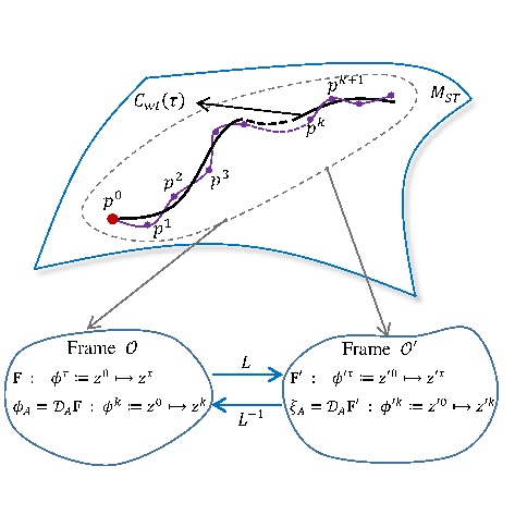
Being both Lorentz covariant and symplectic, an algorithm is of significance in two aspects. In the first place, the preservation of the symplectic structure guarantees that the numerical solutions are good enough to approximate the continuous solutions in arbitrary long time. Secondly, the Lorentz covariance of algorithm makes the numerical results reference-independent, which preserves the geometric nature of original systems. Figure 1 depicts the schematic diagram for the relation between a covariant continuous system and the corresponding discrete systems generated by the Lorentz covariant symplectic algorithm $A$. The 4-spacetime is denoted by $M_{ST}$. The continuous evolution of the original system forms a worldline, marked by $C_{wl}$, starting from the initial condition $p^{0}$. The reference frames $\mathcal{O}$ and $\mathcal{O}^{\prime}$ are two chosen Lorentz inertial frames. For a covariant continuous system, the master equations $\mathbf{F}^{\prime}$ in $\mathcal{O}^{\prime}$ has identical form as $\mathbf{F}$ in $\mathcal{O}$. According to the Lorentz covariance, the solutions of $\mathbf{F}$ and $\mathbf{F}^{\prime}$, i.e., $z^{\tau}$ and $z^{\prime\tau}$, express the same worldline in $M_{ST}$. Given $A$ is a covariant algorithm, the corresponding discretized equations in $\mathcal{O}^{\prime}$ is expressed as $\xi_{A}=\mathcal{D}_{A}\mathbf{F}^{\prime}$, and $\phi_{A}=\mathcal{D}_{A}\mathbf{F}$ denotes the discretized equations in frame $\mathcal{O}$. The sequence determined by $\phi_{A}$ in $\mathcal{O}$ is denoted by $z^{k}$, and the sequence determined by $\xi_{A}$ in $\mathcal{O}^{\prime}$ in denoted by $z^{\prime k}$. According to Eq. 1, we have the relation $\xi_{A}=\mathcal{T}_{L}\phi_{A}$ and thus $z^{\prime k}=\mathcal{T}_{L}z^{k}$ for each proper-time step $k$. Consequently, as the analogy with the continuous case, the numerical results of $A$ in different Lorentz frames provide different numerical solutions $z^{k}$ and $z^{\prime k}$ but the same 4-worldpoint sequence $p^{k}$ in $M_{ST}$. On the other hand, because $A$ is a symplectic algorithm, the conservation of discrete symplectic structure ensures $p^{k}$ locates adjacent to the exact solution of the original continuous system $C_{wl}$ in $M_{ST}$, see the purple curve in Fig. 1. We can conclude that the Lorentz covariant symplectic algorithms have long-term numerical conservativeness, accuracy, and stability, which are independent of the choice of reference frames.

In this section, we introduce a convenient procedure for the construction of LCCSA. The construction of an explicit LCCSA for relativistic dynamics of charged particles is introduced step by step for demonstration. This procedure can be generally applied for the construction of Lorentz covariant symplectic algorithms for any other Lorentz covariant continuous Hamiltonian systems. Since the Lorentz covariance should be preserved during the discretization, the geometric properties in 4-spacetime should be preserved. It is convenient to employ the Lorentz-covariant forms of the continuous system to construct LCCSA.

Firstly, write explicitly down the covariant Hamiltonian equations for charged particles in 4-spacetime. The covariant Hamiltonian describing charged particle dynamics in electromagnetic fields is [21]

where $X^{\alpha}$ is the 4-position vector, $P_{\alpha}$ is the canonical momentum 1-form, and $A_{\alpha}$ denotes the 4-vector-potential 1-form. In Cartesian coordinate system, we have $X^{\alpha}=\left(t,\mathbf{x}\right)$, $P_{\alpha}=\left(\gamma+\phi,-\mathbf{P}\right)$, $A_{\alpha}=\left(\phi,-\mathbf{A}\right)$, and

where $\mathbf{P}$ is the canonical momentum, and $\phi$ and $\mathbf{A}$ are respectively the scalar and vector potentials of electromagnetic fields. Before deriving the Hamiltonian equations, one should notice that the evolution parameters should be Lorentz scalars, which is vital to keep the Lorentz invariance of step-length after discretization. As a direct consideration, we choose the proper time $\tau$ as the evolution parameter. Correspondingly, according to the Hamiltonian given in Eq. 31, we obtain the covariant Hamiltonian equations $\mathbf{F}_{L4}$ [21, 18],

where $\partial_{\alpha}=\partial/\partial X^{\alpha}=\left(\partial/\partial X^{0},\nabla\right)$, $P^{\alpha}=g^{\alpha\beta}P_{\beta}$, and $A^{\alpha}=g^{\alpha\beta}A_{\beta}$. It is readily to see that Eqs. 32 and 33 are geometric equations and have reference invariant forms in all Lorentz inertial frames.

Secondly, discretize the Hamiltonian equations by using a canonical symplectic method. To obtain an explicit scheme with high efficiency, here we choose the Euler-symplectic method, which can be expressed by [17, 9]

where $h$ is the step-length. The Euler-symplectic method does not break the geometric object or the form of continuous equations. Combining Eqs. 32-35, we can obtain the discrete equations of the LCCSA $\phi_{LCCSA}=\mathcal{D}_{LCCSA}\mathbf{F}_{L4}$ as

where $\Delta\tau$ is the step-length of proper time. The difference equations, Eqs. 36-37, act as one-step maps of geometric objects $\left(X^{\alpha,k},P_{\alpha}^{k}\right)\mapsto\left(X^{\alpha,k+1},P_{\alpha}^{k+1}\right)$. As a property of geometric equations, Eqs. 36-37 naturally inherit the reference-independence of Eqs. 32-33. The Lorentz covariance of the LCCSA can also be verified directly through the definition Eq. 1. The Lorentz transformation of $\phi_{LCCSA}$, $\phi_{LCCSA}^{\prime}=\mathcal{T}_{L}\phi_{LCCSA}$, can be given by left-multiplying the Lorentz matrix on both sides of Eqs. 36 and 37. Considering the linear relations of all the terms in Eqs. 36-37, it is obvious to see that $\phi_{LCCSA}^{\prime}$ has the same form with $\xi_{LCCSA}=\mathcal{D}_{LCCSA}\circ\mathcal{T}_{L}\mathbf{F}_{L4}$. Therefore, LCCSA satisfies the definition of Lorentz covariant algorithms.

During discretization, the Lorentz covariance cannot be inherited without keeping geometric objects in 4-spacetime, even though the 4-dimentional covariant Hamiltonian equations are used. To explain this, we provide a counter-example, a non-covariant algorithm (NCOVA) of Eqs. 32-33, namely, $\phi_{NCOVA}$,

where $X^{0}$, $P^{0}$, and $A^{0}$ denote the 0-components of $X^{\alpha}$, $P^{\alpha}$, and $A^{\alpha}$, respectively. The one-step map of $P_{\alpha}$ determined by Eq. 38 is the Euler method. In Eqs. 39-40, the 4-canonical-momentum for pushing $X^{\alpha}$ is treated in different ways. When calculating $X^{0,k+1}$, $P^{0,k+1}$ is used. And $\mathbf{P}^{k}$ is used to calculate $\mathbf{x}^{k+1}$. The integrity of 4-dimentional 1-form $P_{\alpha}$ in Eq. 33 is thus broken, which lead to different forms of Eqs. 39-40 after Lorentz transformations. The bad performance of this NCOVA under Lorentz transformation is presented in numerical examples in Sec. IV, which shows numerically that $\mathcal{T}_{L}\phi_{NCOVA}\neq\xi_{NCOVA}$, where $\xi_{NCOVA}=D_{NCOVA}\circ\mathcal{T}_{L}\mathbf{F}_{L4}$.

In this section, we analyze and test the performances of LCCSA through several numerical experiments.

In this paper, we provide the definition of Lorentz covariant algorithms and introduce Lorentz covariant symplectic algorithms in detail. Lorentz covariant algorithms can generate discretized equations, which inherits the Lorentz covariant nature of original continuous systems. Symplectic algorithms without Lorentz covariance only performs well in one specific inertial frame. While covariant symplectic algorithms are reference-independent and possess long-term conservativeness, which make it convenient and safe to employ the same algorithm in any Lorentz frame. Because of the essentiality of Lorentz covariance, the Lorentz covariant symplectic algorithms have wide applications.

On the other hand, because the time-variable becomes a component of coordinate for 4-spacetime in the construction of LCCSA, the time-dependent Hamiltonian system is no longer a problem for the construction of required symplectic algorithms. Taking the proper time $\tau$ as the dynamical parameter, all time-dependent Hamiltonian system becomes proper-time-independent. The explicit symplectic algorithm, like the LCCSA in Eqs. 36-37, for time dependent systems can be easily constructed. According to the idea and procedure in this paper, many other Lorentz covariant symplectic algorithms as well as other kinds of Lorentz covariant structure-preserving algorithms can be readily constructed. In the future work, we will further investigate the Lorentz covariant structure-preserving algorithms and apply the LCCSAs to study key physical problems.