Markovian nature, completeness, regularity and correlation properties of Generalized Poisson-Kac processes

Massimiliano Giona^∗ Affiliation: Dipartimento di Ingegneria Chimica DICMA Facoltà di Ingegneria, La Sapienza Università di Roma via Eudossiana 18, 00184, Roma, Italy
^∗ Email: massimiliano.giona@uniroma1.it Antonio Brasiello Affiliation: Dipartimento di Ingegneria Industriale Università degli Studi di Salerno via Giovanni Paolo II 132, 84084 Fisciano (SA), Italy Silvestro Crescitelli Affiliation: Dipartimento di Ingegneria Chimica, dei Materiali e della Produzione Industriale Università degli Studi di Napoli “Federico II” piazzale Tecchio 80, 80125 Napoli, Italy

Abstract

We analyze some basic issues associated with Generalized Poisson-Kac (GPK) stochastic processes, starting from the extended notion of the Markovian condition. The extended Markovian nature of GPK processes is established, and the implications of this property derived: the associated adjoint formalism for GPK processes is developed essentially in an analogous way as for the Fokker-Planck operator associated with Langevin equations driven by Wiener processes. Subsequently, the regularity of trajectories is addressed: the occurrence of fractality in the realizations of GPK is a long-term emergent property, and its implication in thermodynamics is discussed. The concept of completeness in the stochastic description of GPK is also introduced. Finally, some observations on the role of correlation properties of noise sources and their influence on the dynamic properties of transport phenomena are addressed, using a Wiener model for comparison.

1 Introduction

Stochastic models find a wide and fertile application in all the fields of physical science. Notwithstanding their ubiquitous application in physics and the huge literature existing on it, some basic issues, alternatives equation setting and, sometimes, misunderstandings in the definition of basic properties are still matter of research and debate [1]. For example, the choice of the most suitable stochastic calculus (Ito, Stratonovich, Klimontovich) in physical applications is still matter of debate [2, 3, 4], although Wong-Zakai theorem [5, 6] and the consistency of a thermodynamic description [7] support the Stratonovich approach (related to this debate see also [8]). Similarly, it is still open the issue of the most appropriate extensions of Brownian motion in a relativistic framework (different model exist, the Relativistic Brownian Motion, the Relativistic Ornstein-Uhlenbeck Process) possessing similar steady-state distributions (the Juttner distribution), but completely different dynamic properties [9]. Sometimes, controversies arise due to the fact the same diction and terminology is used to indicate qualitative different stochastic phenomenologies, and vice versa (as we shall see in the remainder of this article).

Therefore, great attention should be posed in seeking the level of highest clarity in assumptions and definitions, distinguishing between fundamental results of general validity and phenomenologies deriving from particular models, in the strive of constructing a coherent picture of the physical reality upon stochastic models.

This imperative is particularly compelling in contemporary research, at least for two classes of reasons. From one hand, experimental research at micro- and nanoscales permits to obtain accurate measurements of the trajectories of single microsized colloidal particles [10, 11], and to analyze transport phenomena (thermal problems) at extremely short time-scales (picosecond and attosecond physics) [12, 13, 14]. On the other hand, new advancements of non-equilibrium physics (fluctuation-dissipation theorems far from equilibrium [15, 16], stochastic thermodynamics [7], extended thermodynamics [17, 18, 19]), stimulate the research on more general stochastic processes, and their connection with non-equilibrium phenomena, capable of solving the shortcomings and limitations of the existing theories.

This article deals with a class of stochastic processes, the Generalized Poisson-Kac (GPK, for short) processes recently introduced in [21], and their basic properties. GPK processes, briefly reviewed in Section 2, emerge as a generalization of the stochastic model proposed by Mark Kac [20], based on Poissonian fluctuations, representing the stochastic counterpart of the one-dimensional Cattaneo diffusion equation with memory [22]. Poisson-Kac processes solve the unpleasant feature of Wiener processes, and Wiener-driven Langevin equation, of possessing infinite propagation velocity.

In the physical literature, Poisson-Kac processes are known and studied under the dictions of “dichotomous noise”, “two-level bounded noise”, and they have been used essentially as a simple and analytically approachable model of colored noise, because of the exponential decay in time of the correlation function [23, 24, 25, 26, 27, 28, 29]. Although a huge literature has studied the dichotomous noise, the overwhelming majority of the existing contributions deal with one-dimensional spatial models, with the exception of [30] and of a series of significant mathematical works by Kolesnik and coworkers [31, 32, 33, 34] on two-dimensional systems and their complex statistical description.

The importance of Poisson-Kac processes in physics goes far beyond their “colored” (in the meaning of colored noise) applications. As originally observed by Gaveau et al. [35], and subsequently elaborated by other authors [36, 37, 38], Poisson-Kac processes provide a stochastic interpretation to the relativistic Dirac equation for the free electron (in the first paper [35], the one-dimensional Dirac equation is considered), via analytic continuation of the temporal variable. Moreover, under certain conditions, referred to as the Kac limit, Poisson-Kac processes converge to a Langevin equation driven by Wiener fluctuations [20, 39].

These two properties, gathered together, are extremely appealing in theoretical physics (field theories, matter-radiation interaction, fluctuation theory at micro- and nanoscales). On the one hand, all the classical results of stochastic Langevin theory can be recovered (in the Kac limit). On the other hand, the finite propagation velocity characterizing these processes provides a key for the stochastic modeling of electromagnetic fluctuations (zero-point energy, spontaneous emission and adsorption of radiation, etc.). The latter property is relevant in the development of a stochastic field theory of field-matter interactions as the fundamental mechanism of irreversibility and of the exotic properties of matter at the atomic and subatomic scale grounded on stochastic electrodynamics [40, 41, 42, 43].

There is another field in which GPK process can be conveniently used, namely extended thermodynamics [19, 44, 45, 46]. GPK processes provide a firm stochastic ground on the generalization of the thermodynamic formalism referred to as extended thermodynamics of non-equilibrium processes [19, 44, 45], pioneered by Muller and Ruggeri and subsequently elaborated by many other authors, especially Jou, Casas-Vazquez and Lebon [45]. Extended thermodynamic theories represent a highly valuable contribution in generalizing the classical theories of irreversible phenomena [47] essentially in two main directions: (i) by including explicitly thermodynamic fluxes in the representation of the thermodynamic state functions in far-from-equilibrium conditions and, (ii) in connecting this generalization with the requirement of finite propagation velocity. Nevertheless, the existing formulations of extended thermodynamics and the related transport theories still suffer some basic conceptual issues, that should be addressed and solved in order to toughen and make fully consistent the formal apparatus of these theories.

The theory, originated by the Grad 13-moment expansion of the Boltzmann equation [48] is essentially based, as mathematical building block, on the multidimensional Cattaneo equation. In space dimensions higher than one, the Cattaneo equation is not probabilistically consistent, in the meaning that there is no stochastic process for which the Cattaneo equation is the evolution equation for its probability density function. This property implies in turn that the higher-dimensional Cattaneo equation does not preserve non-negativity [49], which is highly unpleasant when this equation is applied to describe the space-time evolution of molecular concentrations, absolute temperature fields, or probability density functions, which by definition attain strictly non-negative values.

Recently, we have started a systematic study of Poisson-Kac processes and of their higher-dimensional extensions (GPK) with the fundamental goals just mentioned above [50, 51, 52, 53, 54]. In developing such a research program, one encounters some delicate issues related to the very basic properties of Poisson-Kac and GPK processes, that require a careful dissection in order to avoid misunderstanding and misinterpretations.

One of this issues is the Markovian nature of these processes. This and related issues are analyzed in the present article. In point of fact, starting from the understanding of general concepts, new formalisms and novel results are developed.

This article is organized as follows. Section 2 briefly reviews GPK processes and their properties that are useful in the remainder. Section 3 discusses their Markovian nature, and from the extended Markovian condition, the adjoint formalism for GPK processes is developed, tracking the analogy with the classical Kolmogorov theory of forward and backward Fokker-Planck equations. Section 4 discusses the emerging fractality of these processes versus their local (short-term regularity), analyzing some of their implications in stochastic energetics (Section 5).

Closely, related to these issues is the concept of completeness of stochastic description, addressed in Section 6. Finally, 7 discussed the role of correlations in Poisson-Kac processes. Comparing a Poisson-Kac dynamics with the evolution of a Langevin equation driven by Wiener fluctuations, possessing the same exponentially decaying correlation function, it is shown that the two model do possess radically different qualitative properties. This observation can be further elaborated in order to describe qualitatively different tunneling phenomenologies in stochastic dynamics.

2 Generalized Poisson-Kac processes

The classical prototype for Poisson-Kac processes is represented by the stochastic differential equation driven by Poisson noise [20], that, in one-dimensional spatial systems, attains the form

dx(t)=v(x(t))\,dt+b\,(-1)^{\chi(t)}\,dt

(1)

where $v(x)$ is a deterministic velocity field, $b>0$ is the characteristic velocity of the stochastic fluctuations, and $\chi(t)$ is a Poisson process possessing transition rate $a>0$ . The stochastic contribution $(-1)^{\chi(t)}$ switches between $+1$ and $-1$ , and this is the reason why this model is often referred to as “dichotomous noise” or “two-level noise” [23, 24, 25, 26, 27]. The initial condition for $\chi(t)$ at $t=0$ is usually set $\chi(0)=0$ with probability 1, as for classical Poisson processes. Alternatively, in order to avoid any form of bias at $t=0$ , it can be set $\chi(0)=0$ and $\chi(0)=1$ with $\mbox{Prob}[\chi(0)=0]=\mbox{Prob}[\chi(0)=1]=1/2$ .

Indicate with $X(t)$ the stochastic process at time $t$ originated by eq. (1), and let

p^{\pm}(x,t)\,dx=\mbox{Prob}[X(t)\in(x,x+dx),\;(-1)^{\chi(t)}=\pm 1\}

(2)

be the associated partial probability densities. The partial probabilities $p^{\pm}(x,t)$ satisfy the balance equations [20, 51]

\partial_{t}p^{\pm}(x,t)=-\partial_{x}\left[v(x)\,p^{\pm}(x,t)\right]\mp b\,\partial_{x}p^{\pm}(x,t)\mp a\,\left[p^{+}(x,t)-p^{-}(x,t)\right]

(3)

In the absence of the deterministic contribution $v(x)$ , the solutions of these equations correspond to waves propagating in the forward ( $p^{+}$ ), and backward ( $p^{-}$ ) $x$ -direction, with mutual recombination controlled by the exponential statistics of the switching times. For this reason, these functions are also referred to as partial probability waves of the Poisson-Kac process. The overall probability density function (pdf) $p(x,t)$ for $X(t)$ at time $t$ is thus given by

p(x,t)=p^{+}(x,t)+p^{-}(x,t)

(4)

In the limit for $a,b\rightarrow\infty$ , keeping fixed and constant the ratio $b^{2}/2a=D$ (where $D$ has the physical dimension of a diffusion constant), the pdf $p(x,t)$ becomes the solution of a classical parabolic advection-diffusion equation

\partial_{t}p(x,t)=-\partial_{x}\left[v(x)\,p(x,t)\right]+D\,\partial_{x}^{2}p(x,t)

(5)

that corresponds to the forward Fokker-Planck equation associated with the Langevin equation

dx(t)=v(x(t))\,dt+\sqrt{2\,D}\,dw(t)

(6)

where $dw(t)$ is the increment in the interval $dt$ of a one-dimensional Wiener process. Eq. (6) represents the Kac limit for eq. (1) while eq. (5) expresses the statistical convergence of the Poisson-Kac process towards the Fokker-Planck equation associated with the Langevin model (6). For further mathematical details on the convergence see [39].

2.1 Generalized Poisson-Kac processes

The Generalized Poisson-Kac processes represent a generalization of eq. (1), particularly suited for modeling stochastic systems in spatial dimensions higher than one [21].

The starting point is the $N$ -state finite Poisson process $\chi_{N}(t)$ , which is a stochastic process attaining, at any $t>0$ , $N$ distinct values $\chi_{N}(t)=1,2,\dots,N$ . As the classical Poisson process, it is a stationary, memoryless and ordinary process, so that in a time interval $\Delta t$ , the transition probabilities from $\chi_{N}(t)=\alpha$ to $\chi_{N}(t+\Delta t)=\beta$ , $\alpha,\beta=1,\dots,N$ , are given by

T_{\alpha\mapsto\beta}(\Delta t)=\lambda_{\alpha}\,A_{\beta,\alpha}\,\Delta t+o(\Delta t)

(7)

and

T_{\alpha\mapsto\alpha}(\Delta t)=\left[1-\lambda_{\alpha}\,\sum_{\beta=1}^{N}A_{\beta,\alpha}\right]\,\Delta t+o(\Delta t)

(8)

where $\lambda_{\alpha}>0$ are the transition rates and ${\bf A}=(A_{\alpha,\beta})_{\alpha,\beta=1}^{N}$ is a left-stochastic matrix,

A_{\beta,\alpha}\geq 0\,,\qquad\sum_{\beta=1}^{N}A_{\beta,\alpha}=1\;\;\;\alpha=1,\dots,N

(9)

Let $\{{\bf b}_{\alpha}\}_{\alpha=1}^{N}$ be a system of $N$ constant vectors of ${\mathbb{R}}^{d}$ , $d=1,2,\dots$ , fulfilling the non-biasing condition $\sum_{\alpha=1}^{N}{\bf b}_{\alpha}=0$ .

A Generalized Poisson Kac process ${\bf X}(t)$ (henceforth GPK) in ${\mathbb{R}}^{d}$ , in the presence of a deterministic velocity field ${\bf v}({\bf x})$ , is defined by the following stochastic differential equation for its realizations ${\bf x}(t)$

d{\bf x}(t)=\left[{\bf v}({\bf x}(t))+{\bf b}(\chi_{N}(t))\right]\,dt

(10)

where

{\bf b}(\chi_{N}(t)=\alpha)={\bf b}_{\alpha}

(11)

and $\chi_{N}(t)$ is a $N$ -state finite Poisson process. Taking into account the properties of $\chi_{N}(t)$ , essentially the fact that it takes only $N$ distinct values, the GPK is fully described by the the conditional probability density functions $p_{\alpha,\beta}({\bf x},t/{\bf y},t_{0})$ , $\alpha,\beta=1,\dots,N$ . Indicating with $d{\bf x}$ the volume element in ${\mathbb{R}}^{d}$ , $p_{\alpha,\beta}({\bf x},t/{\bf y},t_{0})\,d{\bf x}$ , represent the probabilities that ${\bf X}(t)\in({\bf x},{\bf x}+d{\bf x})$ and $\chi_{N}(t)=\alpha$ conditional to ${\bf X}(t_{0})={\bf y}$ and $\chi_{N}(t_{0})=\beta$ , where $t_{0}<t$ ,

	$\displaystyle p_{\alpha,\beta}({\bf x},t/{\bf y},t_{0})\,d{\bf x}$	$\displaystyle=$	$\displaystyle\mbox{Prob}\left[\,{\bf X}(t)\in({\bf x},{\bf x}+d{\bf x})\,,\;\;\chi_{N}(t)=\alpha\right.$		(12)
		$\displaystyle/$	$\displaystyle\left.{\bf X}(t_{0})={\bf y}\,,\;\;\chi_{N}(t_{0})=\beta\,\right]$		(12)

Dropping for notational simplicity the indication about the dependence on the initial state ${\bf y}$ at time $t_{0}$ , the conditional probabilities $p_{\alpha,\beta}({\bf x},t)=p_{\alpha,\beta}({\bf x},t/{\bf y},\beta)$ satisfy the wave-equations

	$\displaystyle\partial_{t}p_{\alpha,\beta}({\bf x},t)$	$\displaystyle=$	$\displaystyle-\nabla_{x}\cdot\left[({\bf v}({\bf x})+{\bf b}_{\alpha})\,p_{\alpha,\beta}({\bf x},t)\right]-\lambda_{\alpha}\,p_{\alpha,\beta}({\bf x},t)$		(13)
		$\displaystyle+$	$\displaystyle\sum_{\gamma=1}^{N}\lambda_{\gamma}\,A_{\alpha,\gamma}\,p_{\gamma,\beta}({\bf x},t)={\mathcal{L}}_{x,\alpha}[p_{\alpha,\beta}({\bf x},t);\{p_{\gamma,\beta}\}_{\gamma=1}^{N}]$		(13)

where $\nabla_{x}$ indicates the nabla-operator with respect to the ${\bf x}$ -variables. The second argument, namely $\{p_{\gamma,\beta}\}_{\gamma=1}^{N}$ , of the operator ${\mathcal{L}}_{x,\alpha}$ , indicates that this operator depends on the whole system of probability densities $p_{1,\beta}({\bf x},t),\dots,p_{N,\beta}({\bf x},t)$ , evaluated at $({\bf x},t)$ corresponding to space-time point of the first argument of ${\mathcal{L}}_{x,\alpha}$ , keeping fixed the second index, namely $\beta$ , of the conditional probabilities. It follows from the structure of eq. (13) that the partial probability waves

\overline{p}_{\alpha}({\bf x},t/{\bf y},t_{0})=\sum_{\beta=1}^{N}p_{\alpha,\beta}({\bf x},t/{\bf y},t_{0})

(14)

defined from the conditional probabilities $p_{\alpha,\beta}({\bf x},t/{\bf y},t_{0})$ , averaging out the information on the initial state of the process $\chi_{N}(t_{0})$ , i.e., summing over $\beta$ , satisfy the same wave equation, namely,

\partial_{t}\overline{p}_{\alpha}({\bf x},t/{\bf y},t_{0})={\mathcal{L}}_{x,\alpha}[\overline{p}_{\alpha}({\bf x},t/{\bf y},t_{0});\{\overline{p}_{\gamma}\}_{\gamma=1}^{N}]

(15)

2.2 A two-dimensional model

Consider the two-dimensional Poisson-Kac process in the absence of deterministic biasing field,

\left\{\begin{array}[]{l}dx(t)=b\,(-1)^{\chi_{1}(t)}\,dt\\ dy(t)=b\,(-1)^{\chi_{2}(t)}\,dt\end{array}\right.

(16)

where $\chi_{1}(t)$ , $\chi_{2}(t)$ are two independent Poisson processes possessing the same statistical properties, namely the same transition rate $a$ . This process can be viewed as a GPK with $N=4$ . In this case, all the $\lambda_{\alpha}$ , $\alpha=1,\dots,4$ coincide and are equal to $2\,a$ . The vectors ${\bf b}_{\alpha}$ are given by: ${\bf b}_{1}=b\,(1,1)$ , ${\bf b}_{2}=b\,(-1,1)$ , ${\bf b}_{3}=b\,(1,-1)$ , ${\bf b}_{4}=b\,(-1,1)$ , where state “ $1$ ” corresponds to $(-1)^{\chi_{1}(t)}=1$ , $(-1)^{\chi_{2}(t)}=1$ , state “2” to $(-1)^{\chi_{1}(t)}=-1$ , $(-1)^{\chi_{2}(t)}=1$ , state “3” to $(-1)^{\chi_{1}(t)}=1$ , $(-1)^{\chi_{2}(t)}=-1$ , state “4” to $(-1)^{\chi_{1}(t)}=-1$ , $(-1)^{\chi_{2}(t)}=-1$ . The transition probability matrix ${\bf A}$ is given by

{\bf A}=\left(\begin{array}[]{llll}0&1/2&1/2&0\\ 1/2&0&0&1/2\\ 0&1/2&1/2&0\\ 1/2&0&0&1/2\end{array}\right)

(17)

The probability of occurrence of the transitions $(-1,-1)\mapsto(1,1)$ or $(1,1)\mapsto(-1,-1)$ in the time interval $\Delta t$ is order of ${\mathcal{O}}(\Delta t^{2})$ , and therefore they are negligible in the limit for $\Delta t\rightarrow 0$ . Observe that in this case ${\bf A}$ is a doubly stochastic matrix. We will use this example, in Section 4 for addressing the regularity of GPK trajectories and the emergent character of their fractal properties.

Similarly, every Poisson-Kac process involving $M$ independent Poisson processes can be viewed as a GPK process involving $N=2^{M}$ states. The reverse property is not necessarily true.

3 Markovian condition and adjoint theory for GPK

The Markovian nature of dichotomous noise processes (and, a fortiori, of GPK) is a controversial issue in the Literature, as some authors have claimed their non-Markovian character [55, 56], while others affirm their Markovian nature [31, 57]. This issue is essentially of semantical nature, albeit it disclosures relevant consequences in the development of the GPK theory.

In some sense - paraphrasing Plato - the Markovian nature of a process “lies in the eye of the beholder”, as it depends essentially on the way it is defined. Intuitively, the Markovian character of a process accounts for its memoryless property, in that the complete statistical information on the process at any given time $t_{0}$ is fully sufficient to achieve a complete statistical knowledge of the process at any later time $t>t_{0}$ .

This is the essence of the Markov condition, albeit the last sentence disclosures a delicate issue, related to the formal and exact meaning of the concept of “complete statistical description”. A typical example of this apparent ambiguity is represented by the concept of Markovian embedding [58].

Consider a Langevin equation of the form

dx(t)=v(x(t),w(t))\,dt+a(x(t),w(t))\,dw(t)

(18)

where $w(t)$ is a one-dimensional Wiener process, and the coefficients $v(x,w)$ , $a(x,w)$ depend not solely on the process $X(t)$ at time $t$ , but also on the stochastic perturbation $W(t)$ at the same time $t$ . This process is strictly-speaking, non Markovian, as the probability density function $p(x,t)$ does not satisfy the Markovian condition

p(x,t+\tau/x_{0},t_{0})=\int p(x,t+\tau/y,t)\,p(y,t/x_{0},t_{0})\,dy

(19)

where $t_{0}<t$ and $\tau>0$ . Next, introduce the auxiliary process $Y(t)=W(t)$ , i.e.,

dy(t)=dw(t)

(20)

with $y(0)=0$ . With this extension, the vector-valued stochastic process ${\bf X}(t)=(X(t),Y(t))$ the dynamics of which is expressed by eq. (20) and by eq. (18), which now can be rewritten as

dx(t)=v(x(t),y(t))\,dt+a(x(t),y(t))\,dw(t)

(21)

is Markovian. This is the essence of the technique of Markovian embedding [58], and of the concept of generalized (hidden) Markov processes [59, 60], which is conceptually similar either to the concept of suspension for deterministic non-autonomous systems, in order to transform them in autonomous ones by adding an additional phase-space coordinate homeomorphic to time [61], and to the deterministic embedding of attractors due to Takens [62], in order to reconstruct a chaotic attractor from a single time series.

Keeping in mind the essential meaning of the Markov property, namely that the statistical knowledge of a process at time $t$ is fully determined by its statistical information at any preceding time $t_{0}<t$ , and it is immaterial of its history preceding $t_{0}$ , a Markov condition can be stated also for GPK, bearing in mind that all the statistical information needed to describe the system is contained in the conditional probability densities $\{p_{\alpha,\beta}({\bf x},t/{\bf y},t_{0})\}_{\alpha,\beta=1}^{N}$ that keep also track of the state of the $N$ -state finite Poisson process generating the randomness in the system.

In order to avoid confusion with the concept of generalized Markovian processes, it is convenient to introduce the definition of extended Markovian processes.

A stochastic vector-valued process ${\bf Z}(t)$ is said to be an extended Markovian process if: (i) there exist $M>0$ non-negative functions $\pi_{k}({\bf z},t/{\bf z}_{0},t_{0})$ such that the conditional probability density $p({\bf z},t/{\bf z}_{0},t_{0})$ of finding the state of the process in ${\bf z}$ at time $t$ , given the initial state ${\bf z}_{0}$ at time $t_{0}<t$ is given by

p({\bf z},t/{\bf z}_{0},t_{0})=\sum_{k=1}^{M}\pi_{k}({\bf z},t/{\bf z}_{0},t_{0})

(22)

and (ii) there exits $M^{3}$ non-negative constants $C_{k}^{p,q}$ such that the functions $\pi_{k}({\bf z},t/{\bf z}_{0},t_{0})$ satisfy the recurrence equation for any ${\bf z},\,{\bf z}_{0}$ and $t_{0}<t_{1}<t$ ,

\pi_{k}({\bf z},t/{\bf z}_{0},t_{0})=\sum_{p,q=1}^{M}C_{k}^{p,q}\int\pi_{p}({\bf z},t/{\bf y},t_{1})\,\pi_{q}({\bf y},t_{1}/{\bf z}_{0},t_{0})\,d{\bf y}

(23)

Horsthemke and Lefevre [24] have proved that the extended Markovian property holds for the one-dimensional Poisson-Kac model eq. (1) driven by dichotomous Poisson noise. In the setting of GPK processes, the Horsthemke-Lefevre condition becomes (for $t_{1}<t_{2}<t_{3})$ ,

p_{\alpha,\beta}({\bf x},t_{3}/{\bf z},t_{1})=\sum_{\gamma=1}^{N}\int p_{\alpha,\gamma}({\bf x},t_{3}/{\bf y},t_{2})\,p_{\gamma,\beta}({\bf y},t_{2}/{\bf z},t_{1})\,d{\bf y}

(24)

$\alpha,\beta=1,\dots,N$ . Enforcing the transition properties of a $N$ -time finite Poisson process, it is straightforward to derive the balance equation eq. (13) from the extended Markovian relation (24). The technique is essentially analogous to that used in [24] and its is not repeated here.

In point of fact, eq. (24) corresponds to the extended Markov property defined by eq. (23) where the conditional probability densities $\{p_{\alpha,\beta}\}_{\alpha,\beta=1}^{N}$ play the role of the $M=N^{2}$ auxiliary functions $\{\pi_{k}\}_{k=1}^{M}$ . Eq. (24) can be thus rewritten in the form of eq. (23), i.e.,

p_{\alpha,\beta}({\bf x},t_{3}/{\bf z},t_{1})=\sum_{\gamma,\epsilon,\zeta,\xi=1}^{N}C_{(\alpha,\beta)}^{(\gamma,\epsilon),(\zeta,\xi)}\int p_{\gamma,\epsilon}({\bf x},t_{3}/{\bf y},t_{2})\,p_{\zeta,\xi}({\bf y},t_{2}/{\bf z},t_{1})\,d{\bf y}

(25)

by introducing the coefficient tensor $C_{(\alpha,\beta)}^{(\gamma,\epsilon),(\zeta,\xi)}=\delta_{\alpha}^{\gamma}\,\delta_{\beta}^{\xi}\,\delta^{\epsilon,\zeta}$ , where $\delta_{\alpha}^{\gamma}$ , $\delta^{\epsilon,\zeta}$ are the Kronecker symbols, written in countervariant and mixed way purely because of notational index consistency.

3.1 Adjoint formalism and first transit-time statistics

A mathematical definition is useful in physics if, starting from it, it is possible to derive physical consequences on the process under investigation. This is the case of the extended Markov property that permits to derive the adjoint formalism for GPK processes and the first-transit description, conceptually analogous to that of strictly Markovian processes associated with Langevin equations driven by Wiener fluctuations.

Consider eqs. (24), where the probabilities $p_{\alpha,\beta}({\bf x},t_{3}/{\bf z},t_{1})$ satisfies the forward evolution equations (13), below rewritten for convenience

\partial_{t_{2}}p_{\gamma,\beta}({\bf y},t_{2}/{\bf z},t_{1})={\mathcal{L}}_{y,\gamma}[p_{\gamma,\beta}({\bf y},t_{2}/{\bf z},t_{1});\{p_{\xi,\beta}\}_{\xi=1}^{N}]

(26)

Summing in eq. (24) over the indexes $\alpha,\,\beta$ , and integrating over ${\bf x}$ , the identity follows

1=\sum_{\alpha,\beta,\gamma=1}^{N}\int d{\bf x}\int d{\bf y}\,p_{\alpha,\gamma}({\bf x},t_{3}/{\bf y},t_{2})\,p_{\gamma,\beta}({\bf y},t_{2}/{\bf z},t_{1})

(27)

Taking the derivative with respect to $t_{2}$ and enforcing the forward evolution equation (26) for $p_{\gamma,\beta}({\bf y},t_{2}/{\bf z},t_{1})$ , one obtains

	$\displaystyle 0$	$\displaystyle=$	$\displaystyle\sum_{\alpha,\beta,\gamma=1}^{N}\int d{\bf x}\int d{\bf y}\left[p_{\gamma,\beta}({\bf y},t_{2}/{\bf z},t_{1})\,\partial_{t_{2}}p_{\alpha,\gamma}({\bf x},t_{3}/{\bf y},t_{2})\right.$		(28)
		$\displaystyle+$	$\displaystyle\left.p_{\alpha,\gamma}({\bf x},t_{3}/{\bf y},t_{2})\,{\mathcal{L}}_{y,\gamma}[p_{\gamma,\beta}({\bf y},t_{2}/{\bf z},t_{1});\{p_{\xi,\beta}\}_{\xi=1}^{N}]\right]$		(28)

Consider the space $L^{2}_{N}({\mathbb{R}}^{d})$ of $N$ -dimensional vector-valued square summable functions in ${\mathbb{R}}^{d}$ attaining real values as, in our case, probability densities are involved. This is a Hilbert space equipped with the inner product $(\cdot,\cdot)_{L^{2}_{N}}$ : if ${\bf f}({\bf x})=(f_{1}({\bf x}),\dots,f_{N}({\bf x}))$ , ${\bf g}({\bf x})=(g_{1}({\bf x}),\dots,g_{N}({\bf x}))$ belong to $L^{2}_{N}({\mathbb{R}}^{d})$ , then

({\bf f},{\bf g})_{L^{2}_{N}}=\sum_{\gamma=1}^{N}\int f_{\gamma}({\bf x})\,g_{\gamma}({\bf x})\,d{\bf x}

(29)

In eq. (28), the integral over ${\bf y}$ and the sum over $\gamma$ can be viewed as a scalar product in ${L^{2}_{N}}({\mathbb{R}}^{d})$ of the transforms of the two functions ${\bf f}({\bf y},t_{2})$ and ${\bf g}({\bf y},t_{2})$ , the entries of which are given by

f_{\gamma}({\bf y},t_{2})=\sum_{\alpha=1}^{N}p_{\alpha,\gamma}({\bf x},t_{3}/{\bf y},t_{2})

(30)

and

g_{\gamma}({\bf y},t_{2})=\sum_{\beta=1}^{N}p_{\gamma,\beta}({\bf y},t_{2}/{\bf z},t_{1})

(31)

$\gamma=1,\dots,N$ , upon the action of the differential operators $\partial_{t_{2}}$ and $\{{\mathcal{L}}_{y,\gamma}\}_{\gamma=1}^{N}$ (the dependence on ${\bf x}$ , $t_{3}$ , ${\bf z}$ , $t_{1}$ has been omitted for notational simplicity), respectively. Therefore, eq. (28) can be expressed as

0=\int d{\bf x}\left[(\partial_{t_{2}}{\bf f},{\bf g})_{L^{2}_{N}}+({\bf f},\widehat{{\mathcal{L}}}_{y}[{\bf g}])_{L^{2}_{N}}\right]

(32)

where $\widehat{{\mathcal{L}}}_{y}$ is the vector-valued extension of the $N$ differential linear operators ${\mathcal{L}}_{y,\alpha}$

\widehat{{\mathcal{L}}}_{y}=\left(\begin{array}[]{c}{\mathcal{L}}_{y,1}\\ {\mathcal{L}}_{y,2}\\ \cdot\\ \cdot\\ {\mathcal{L}}_{y,N}\end{array}\right)\,.

(33)

Let $\widehat{{\mathcal{L}}}_{y}^{+}$ be the adjoint of $\widehat{{\mathcal{L}}}_{y}$ , which is simply the vector-valued extension of the adjoints ${\mathcal{L}}_{y,\alpha}^{+}$ of the operators ${\mathcal{L}}_{y,\alpha}$ ,

\widehat{{\mathcal{L}}}_{y}^{+}=\left(\begin{array}[]{c}{\mathcal{L}}_{y,1}^{+}\\ {\mathcal{L}}_{y,2}^{+}\\ \cdot\\ \cdot\\ {\mathcal{L}}_{y,N}^{+}\end{array}\right)

(34)

Eq. (32) thus becomes

0=\int d{\bf x}\left[(\partial_{t_{2}}{\bf f},{\bf g})_{L^{2}_{N}}+(\widehat{{\mathcal{L}}}_{y}^{+}[{\bf f}],{\bf g})_{L^{2}_{N}}\right]=\int d{\bf x}\,(\partial_{t_{2}}{\bf f}+\widehat{{\mathcal{L}}}_{y}^{+}[{\bf f}],{\bf g})_{L^{2}_{N}}

(35)

and since it should be valid for any ${\bf g}$ , it implies that

\partial_{t_{2}}{\bf f}+\widehat{{\mathcal{L}}}_{y}^{+}[{\bf f}]=0

(36)

The entries of the vector-valued function ${\bf f}({\bf y},t_{2})$ are, by definition eq. (30), the backward-in-time partial probability waves

f_{\gamma}({\bf y},t_{2})=\sum_{\alpha=1}^{N}p_{\alpha,\gamma}({\bf x},t_{3}/{\bf y},t_{2})=\overline{p}_{\gamma}^{(b)}({\bf x},t_{3}/{\bf y},t_{2})

(37)

(the summation involves the first inder $\alpha$ of $p_{\alpha,\gamma}$ ), so that eq. (36) can be expressed as

\partial_{t_{2}}\overline{p}_{\gamma}^{(b)}({\bf x},t_{3}/{\bf y},t_{2})+{\mathcal{L}}_{y,\gamma}^{+}[\overline{p}_{\gamma}^{(b)}({\bf x},t_{3}/{\bf y},t_{2});\{\overline{p}_{\beta}^{(b)}\}_{\beta=1}^{N}]=0

(38)

which is the evolution equation, reversed in time, for the backward-in-time partial probability waves. Due to the linearity of the definition of the partial waves $\overline{p}_{\gamma}^{(b)}({\bf x},t_{3}/{\bf y},t_{2})$ eq. (37), and the independence of the equation (38) of the final state $\alpha$ , the same equation applies to each individual term $p_{\alpha,\gamma}({\bf x},t_{3}/{\bf y},t_{2})$ , namely

\partial_{t_{2}}p_{\alpha,\gamma}({\bf x},t_{3}/{\bf y},t_{2})+{\mathcal{L}}_{y,\gamma}^{+}[p_{\alpha,\gamma}({\bf x},t_{3}/{\bf y},t_{2});\{p_{\alpha,\beta}\}_{\beta=1}^{N}]=0

(39)

where by eq. (13) the adjoint operator ${\mathcal{L}}_{y,\gamma}^{+}$ , $\gamma=1,\dots,N$ , are given by

	$\displaystyle{\mathcal{L}}_{x,\gamma}^{+}[p_{\alpha,\gamma}({\bf x},t);\{p_{\alpha,\beta}\}_{\beta=1}^{N}]$	$\displaystyle=$	$\displaystyle({\bf v}({\bf x})+{\bf b}_{\gamma})\cdot\nabla_{x}\,p_{\alpha,\gamma}({\bf x},t)-\lambda_{\gamma}\,p_{\alpha,\gamma}({\bf x},t)$		(40)
		$\displaystyle+$	$\displaystyle\sum_{\beta=1}^{N}\lambda_{\gamma}\,A_{\beta,\gamma}\,p_{\alpha,\beta}({\bf x},t)$		(40)

where we have set, for notational simplicity, $p_{\alpha,\gamma}({\bf x},t)=p_{\alpha,\gamma}({\bf z},\tau/{\bf x},t)$ , for generic ${\bf z}$ and $\tau$ .

3.2 First transit-time statistics

The analysis of first transit times for dichotomous noise has been developed in several articles, almost exclusively considering the case of one-dimensional spatial problems [55, 63, 64, 65, 66, 67, 68, 69]. The general formulation of this analysis does not exists for GPK, and consequently it is developed below in the most general setting.

Consider the first transit-time probability density functions. For GPK processes, $N$ such probability densities can be defined $\widehat{F}_{\beta}({\bf x}/{\bf y},t)$ , $\beta=1,\dots,N$ , where $\widehat{F}_{\beta}({\bf x}/{\bf y},t)$ is the probability density function for the first transit-time through ${\bf x}$ , given the initial state ${\bf y}$ at time $t=0$ and $\chi_{N}(0)=\beta$ . The definition of $\widehat{F}_{\beta}({\bf x}/{\bf y},t)$ implicitly assume that, starting from ${\bf y}$ at time $t=0$ , there is a trajectory of the process that reaches ${\bf x}$ in finite time. This is in general not true for all ${\bf x}$ and ${\bf y}$ , in the presence of deterministic biasing field, as the analysis developed in [51] illustrates. Under the above hypothesis, by definition

\int_{0}^{\infty}\widehat{F}_{\beta}({\bf x}/{\bf y},t)\,dt=1

(41)

The density function $\widehat{F}_{\beta}({\bf x}/{\bf y},t)$ can be dissected also with respect to the final state of the process $\chi_{N}(t)$ at the transit time $t$ as

\widehat{F}_{\beta}({\bf x}/{\bf y},t)=\sum_{\alpha=1}^{N}F_{\alpha,\beta}({\bf x}/{\bf y},t)

(42)

where $F_{\alpha,\beta}({\bf x}/{\bf y},t)$ corresponds to the transit-time probability density of passing through ${\bf x}$ at time $t$ with $\chi_{N}(t)=\alpha$ , starting from ${\bf y}$ at time $t=0$ , given that $\chi_{N}(0)=\beta$ .

The introduction of these quantities permits to derive easily an equation for $\widehat{F}_{\beta}({\bf x}/{\bf y},t)$ , using essentially the same strategy adopted in the strictly Markovian case. Indeed, the conditional probabilities $p_{\alpha,\beta}({\bf x},t/{\bf y},0)$ can be expressed in terms of $F_{\alpha,\beta}({\bf x}/{\bf y},t)$ for $t>0$ as

p_{\alpha,\beta}({\bf x},t/{\bf y},0)=\sum_{\gamma=1}^{N}\int_{0}^{t}F_{\gamma,\beta}({\bf x}/{\bf y},t-\tau)\,p_{\alpha,\gamma}({\bf x},\tau/{\bf x},0)\,d\tau

(43)

$\alpha,\beta=1,\dots,N$ . Eqs. (43) correspond to the fact that the probability $p_{\alpha,\beta}({\bf x},t/{\bf y},0)$ is the integral over time $\tau$ , from $\tau=0$ to the current time $\tau=t$ , and the sum over all the possible states $\gamma$ , from $1$ to $N$ , of the probability of arriving for the first time in ${\bf x}$ , starting from ${\bf y}$ and $\chi_{N}(0)=\beta$ at time $t-\tau$ with $\chi_{N}(t-\tau)=\gamma$ , which is $F_{\gamma,\beta}({\bf x}/{\bf y},t-\tau)$ , times the probability that in the remaining time $\tau$ the system will return to ${\bf x}$ , i.e., $p_{\alpha,\gamma}({\bf x},\tau/{\bf x},0)$ .

But,

p_{\alpha,\beta}({\bf x},t/{\bf y},0)=p_{\alpha,\beta}({\bf x},0/{\bf y},-t)

(44)

and, because of eq. (39), this quantity satisfies the backward equation

\partial_{t}p_{\alpha,\beta}({\bf x},t/{\bf y},0)-{\mathcal{L}}_{y,\beta}^{+}[p_{\alpha,\beta}({\bf x},t/{\bf y},0);\{p_{\alpha,\xi}\}_{\xi=1}^{N}]=0

(45)

Consequently, the function at the r.h.s. of eq. (43) satisfies eq. (45) with respect to ${\bf y}$ , and its direct substitution into the latter equation provides the expression

	$\displaystyle\sum_{\gamma=1}^{N}F_{\gamma,\beta}({\bf x}/{\bf y},0)\,p_{\alpha,\gamma}({\bf x},t/{\bf y},0)+\sum_{\gamma=1}^{N}\int_{0}^{t}\left\{\partial_{t}F_{\gamma,\beta}({\bf x}/{\bf y},t-\tau)\right.$
	$\displaystyle-\left.{\mathcal{L}}_{y,\beta}^{+}[F_{\gamma,\beta}({\bf x}/{\bf y},t-\tau);\{F_{\gamma,\xi}\}_{\xi=1}^{N}]\right\}\,p_{\alpha,\gamma}({\bf x},\tau/{\bf x},0)\,d\tau=0$		(46)

For any ${\bf x}\neq{\bf y}$ , $F_{\gamma,\beta}({\bf x}/{\bf y},0)=0$ , and since eq. (46) should be valid for any ${\bf x}$ , it implies that the integrand under parenthesis should be identically vanishing. This returns the equation for $F_{\gamma,\beta}({\bf x}/{\bf y},t)$ as a function of $t$ and of the initial state ${\bf y}$ ,

\partial_{t}F_{\gamma,\beta}({\bf x}/{\bf y},t)={\mathcal{L}}_{y,\beta}^{+}[F_{\gamma,\beta}({\bf x}/{\bf y},t);\{F_{\gamma,\xi}\}_{\xi=1}^{N}]

(47)

which is a backward equation governed by the adjoint operator ${\mathcal{L}}_{y,\beta}^{+}$ of the initial state of the process $\chi_{N}(0)$ , i.e., $\beta$ . Summing over $\gamma$ , an analogous equation for $\widehat{F}_{\beta}({\bf x}/{\bf y},t)$ is obtained,

\partial_{t}\widehat{F}_{\beta}({\bf x}/{\bf y},t)={\mathcal{L}}_{y,\beta}^{+}[\widehat{F}_{\beta}({\bf x}/{\bf y},t),\{\widehat{F}_{\alpha}\}_{\alpha=1}^{N}]

(48)

which is the relevant equation for practical calculations.

Next, consider the moment hierarchy of the first transit-times $\{T_{\beta}^{(n)}({\bf x}/{\bf y})\}_{\beta=1}^{N}$ , $n=0,\dots,N$ . For simplicity, we drop the dependence on the final state ${\bf x}$ , rewriting $T_{\beta}^{(n)}({\bf x}/{\bf y})$ simply as $T_{\beta}^{(n)}({\bf y})$ ,

T_{\beta}^{(n)}({\bf y})=\int_{0}^{\infty}t^{n}\,\widehat{F}_{\beta}({\bf x}/{\bf y},t)\,dt

(49)

From eq. (48) one obtains the system of equations for $T_{\beta}^{(n)}({\bf y})$

{\mathcal{L}}_{y,\beta}^{+}[T_{\beta}^{(n)}({\bf y});\{T_{\alpha}^{(n)}\}_{\alpha=1}^{N}]+n\,T_{\beta}^{(n)}({\bf y})=0

(50)

Since $T_{\beta}^{(0)}({\bf y})=1$ , the equations for the mean first-transit times become

{\mathcal{L}}_{y,\beta}^{+}[T_{\beta}^{(1)}({\bf y}),\{T_{\alpha}^{(1)}\}_{\alpha=1}^{N}]+1=0

(51)

and the average mean first-transit time $\langle T^{(1)}({\bf y})\rangle$ is the weighted average of the $T_{\beta}^{(1)}({\bf y})$ with respect to the initial probabilities $\pi_{\beta}=\mbox{Prob}[\chi_{N}(0)=\beta]$

\langle T^{(1)}({\bf y})\rangle=\sum_{\beta=1}^{N}\pi_{\beta}\,T_{\beta}^{(1)}({\bf y})

(52)

Eqs. (50) are equipped with the boundary condition $T_{\beta}^{(n)}({\bf x})=0$ for $n\geq 1$ .

3.3 A simple example

In this paragraph we do not consider any specific physical problem involving the estimate of the mean first-transit times, but rather a very simple - the simplest - example that highlights the wave-like nature of GPK and the role of boundary conditions.

Consider the mean first transit-time at $x=1$ for a pure Poisson-Kac diffusion problem in $[0,1]$ where the boundary at $x=0$ is impermeable to transport. The stochastic model is thus

dx(t)=b\,(-1)^{\chi(t)}\,dt

(53)

where the Poisson process $\chi(t)$ is characterized by the transition rate $a$ . Let $\alpha=1$ be the state characterized by $(-1)^{\chi(t)}=1$ , and $\alpha=2$ the other state $(-1)^{\chi(t)}=-1$ , and use the notation $T^{(+)}(y)=T_{1}^{(1)}(y)$ , and $T^{(-)}(y)=T_{2}^{(1)}(y)$ . The equations for $T^{(\pm)}(y)$ in the present case follows from eq. (51)

	$\displaystyle b\,\frac{dT^{(+)}(y)}{dy}-a\,T^{(+)}(y)+a\,T^{(-)}(y)+1$	$\displaystyle=$	$\displaystyle 0$
	$\displaystyle-b\,\frac{dT^{(-)}(y)}{dy}+a\,T^{(+)}(y)-a\,T^{(-)}(y)+1$	$\displaystyle=$	$\displaystyle 0$		(54)

equipped with reflecting boundary conditions at $x=0$ ,

T^{(-)}(0)=T^{(+)}(0)

(55)

and with the exit conditions at $y=1$ ,

T^{(+)}(1)=0\,,\qquad T^{(-)}(1)=0

(56)

Equations (55) have been derived by several authors in the one-dimensional case of Poissonian dichotomous noise [63, 64, 65, 66], considering also the effect of potential fields and energy barriers. Here, we are not interested in the physics of transition rates, but essentially on the undulatory mechanism of the propagation of Poisson-Kac dynamics and of its phenomenological implications.

From the wave-like nature of the process, solely the condition for $T^{(+)}(y)$ at $y=1$ propagates, as the first equation (54) represents a backward wave with respect to the initial position $y$ . Consequently, $T^{(+)}(y)$ is a continuous function of $y$ , propagating the transit-time condition $T^{(+)}(1)=0$ smoothly up to the reflecting boundary, located at $y=0$ . This is not the case of $T^{(-)}(y)$ . As $T^{(-)}(y)$ describes the mean first-transit time through $y=1$ , starting from the initial state $(-1)^{\chi(0)}=-1$ , in order to reach $y=1$ , a particle must travel, first backwardly in space, and solely after the first switching of the stochastic Poisson process - that can occur either because of the internal Poissonian recombination between forwardly and backwardly directed perturbations, or because of the reflection at $y=0$ - it can travel in the direction of positive $y$ and reach the exit point located at $y=1$ . This explains the behavior of $T^{(+)}(y)$ and $T^{(-)}(y)$ depicted in figure 1. Focusing attention on $T^{(-)}(y)$ , which is the most interesting quantity, this function is discontinuous at the exit point $y=1$ , as $T^{(-)}(1)=0$ , but the left limit is different from zero, $\lim_{y\rightarrow 1^{-}}T^{(-)}(y)\neq 0$ .

Refer to caption — Figure 1: Behavior of $T^{(+)}(y)$ (line a) and $T^{(-)}(y)$ (line b) vs $y$ in the case of the pure Poisson-Kac stochastic process (53) with $a=1$ and $D=1$ . The lines represent the solution of eqs. (54) with the boundary conditions (55)-(56).

Moreover, it follows from the above observations, that $T^{(-)}(y)$ does not need to be a monotonic function of $y$ . Backwardly oriented particles, initially placed say at $y_{1}$ , can reach sooner the exit point $y=1$ than particles initially located closer to the exit points, i.e., at $y_{2}>y_{1}$ , due to the recombination/reflection mechanism described above.

To complete the picture, figure 2 depicts the comparison of the solution of the first transit-time problem (54)-(56) with Monte-Carlo simulations. These simulations have been performed integrating eq. (54) with a time step $h_{t}=10^{-3}$ , using an ensemble of $10^{5}$ particles for each initial position. Fixing $D=1$ , non-monotonicity of $T^{(-)}(y)$ occurs for values of $a$ close to $1$ . For very low values of $a$ (line (a) in panel (b)). the profile of $T^{(-)}(y)$ , is a monotonically increasing function of $y$ , meaning that the exit through $y=1$ is controlled by reflections at $y=0$ . Conversely, for values of $a\gg 1$ , internal recombination effect prevails, and $dT^{(-)}(y)/dy<0$ .

Observe that $T^{(+)}(y)$ and $T^{(-)}(y)$ are in general radically different from each other, so that the estimate of the mean transit time $\langle T^{(1)}(y)\rangle$ via eq. (52) depends significantly on the probability weights $\pi_{\beta}$ , $\beta=1,\dots,N$ , i.e., on the state of the noise perturbation at time $t=0$ .

4 Smoothness of trajectories and emergent fractal properties

The most remarkable property of Poisson-Kac and GPK processes is their intrinsic trajectory smoothness, provided that the rates $\{\lambda_{\alpha}\}_{\alpha=1}^{N}$ and the norms of the characteristic velocity vectors $\left\{\bf b\right\}_{\alpha=1}^{N}$ are bounded. This means that, with probability $1$ , the trajectories of these processes are almost everywhere differentiable function of time $t$ . Differentiability is lost at any time instant, say $t^{*}$ , when a transition from a state $\alpha$ to a state $\beta$ occurs, but these time instants form a countable sequence (with probability $1$ ) and, in any case, left and right velocities can be defined at $t^{*}$ , such that

\frac{d{\bf x}(t^{*}_{+})}{dt}-\frac{d{\bf x}(t^{*}_{-})}{dt}={\bf b}_{\beta}-{\bf b}_{\alpha}

(57)

Smoothness marks a deep distinction with respect to Langevin equations driven by Wiener processes, which possess fractal trajectories characterized by a fractal dimension $d_{T}=3/2$ [70].

Notwithstanding this basic property, purely diffusive GPK processes possess emergent fractal properties, for any bounded values of the rate and velocity parameters, analogous to those characterizing the corresponding Wiener-driven diffusive counterparts. We define purely diffusive, any GPK process driven exclusively by unbiased ( $\sum_{\alpha=1}^{N}{\bf b}_{\alpha}=0$ ) stochastic perturbations, such that the deterministic component of the dynamics is absent, ${\bf v}({\bf x})=0$ , in eq. (10), and such that a Kac limit exists [21].

This means that a form of “convergence” towards the classical Brownian behavior can be observed at sufficiently long-times, for any values of the parameters.

In order to highlight this result using a physically interesting example, we analyze the case of a two-dimensional Poisson-Kac diffusion in a confined geometry represented by a deterministic fractal structure. Subsequently we analyze the implications of the emergent fractality considering a pattern formation problem arising from colloidal aggregation theory [71]. Poisson-Kac stochastic processes on fractals have been studied in [52]. The content of paragraph 4.1 is therefore a succinct review of the analysis developed in [52], albeit using different fractal models, to avoid repetition. Although, some degree of overlapping exists between the content of paragraph 4.1 and the analysis is [52], this review is nonetheless functional to the novel analysis developed in paragraph 4.2, and further in 5.

4.1 Poisson-Kac diffusion on fractals

Consider the two-dimensional Poisson-Kac model (16). In the Kac limit, it converges to a pure Brownian diffusion process characterized by a diffusion coefficient $D=b^{2}/2a$ . Set $D=1$ . This means that, for any value of $a$ , the characteristic velocity $b$ attains the value $b=\sqrt{2\,a}$ .

Instead of analyzing how fractality of Poisson-Kac trajectories originates in free-space propagation, consider the same problem in a deterministic two-dimensional fractal structure, which is physically more appealing.

The model structure considered is depicted in figure 3. It is a loopless fractal that can be generated using $N_{t}=9$ affine transformations rescaling the length by a factor of $4$ . Its fractal dimension is therefore, $d_{f}=\log 9/\log 4\simeq 1.584$ .

Brownian diffusion in fractal structure is anomalous [72, 73], meaning that the mean square displacement $\langle r^{2}(t)\rangle$ of Brownian particles scales with time $t$ as

\langle r^{2}(t)\rangle\sim t^{2/d_{w}}

(58)

where $d_{w}>2$ is the walk dimension. Since the fractal structure considered is loopless and possesses a chemical dimension $d_{C}=1$ [72], the classical theory of transport on fractals provides for $d_{w}$ the expression [72, 73]

d_{w}=d_{f}+1\simeq 2.584

(59)

Consider the Poisson-Kac diffusion process (16) in this structure. To be precise, the structure considered is depicted in figure 3 (c), and consists of the sixth-iteration pre-fractal in the construction process. We assume that the elementary unit of this structure possesses unit size (figure 3 (a)), so that the sixth iteration possesses a maximum length size $L_{\rm max}^{(6)}=4096$ , as depicted in figure 3 (c).

Poisson-Kac diffusion is simulated in an off-lattice way, by integrating eq. (16) starting from a point chosen at random inside the fractal structure. Reflection conditions are assumed at the boundary of the fractal set. Figure 4 depicts a portion of the orbit of a Poisson-Kac particle at $a=1$ . The orbit is almost everywhere smooth, and discontinuity in the velocity arise as a consequences either of the internal Poissonian switching or of the reflection at the boundary [52]. At longer time-scales, this regularity is broken as a consequence of the two mechanisms mentioned above, and the anomalous features of Brownian motion can be recovered as a long-term property.

Instead of performing the classical analysis of the mean square displacement, consider a trajectory-based approach, consisting in characterizing the anomalous transport properties using the length-resolution analysis of Poisson-Kac trajectories. Take the trajectory of a Poisson-Kac particle, obtained by integrating eq. (16) from time $t=0$ up to $t=t_{\rm max}$ . We use $h_{t}$ as the integration step of eq. (16), and $t_{\rm max}=h_{t}\times(4096)^{2}$ . Let $L(\Delta t)$ be the length of this portion of a trajectory estimated by sampling it with a sampling time $\Delta t\geq h_{t}$ . For a fractal curve [74]

L(\Delta t)\sim\Delta t^{1-d_{T}}=\Delta t^{H-1}\,,

(60)

where $d_{T}$ is the trajectory dimension and $H$ its Hölder exponent, related to $d_{T}$ by the equation $d_{T}=2-H$ .

Since $H=1/d_{w}$ , it is possible to estimate the walk dimension $d_{w}$ (and consequently the basic anomalous features of transport in fractals) enforcing the length-resolution analysis, using the relation

L(\Delta t)\sim\Delta t^{1/d_{w}-1}

(61)

Figure 5 depicts the results of this analysis for two values of $a=1,\,10$ . As expect, at higher resolutions (small $\Delta t$ ), $L(\Delta t)\rightarrow\mbox{constant}$ , due to the regularity of the trajectories (implying $d_{T}=1$ , and ballistic motion $d_{w}=1$ ). Above a crossover resolution $\Delta t_{c}$ , which depends on $a$ , the fractal scaling eq. (61) appears, and the value of $d_{w}$ predicted by eq. (61) nicely agrees with the theoretical estimate of $d_{w}$ given by eq. (59), namely $1-1/d_{w}\simeq 0.613$ .

To conclude, even in the presence of complex geometrical constraints, Poisson-Kac processes equipped with reflecting boundary conditions approach in the long-term limit the characteristic fractal behavior typical of Brownian particles diffusing in the same structures.

In the cases of Poisson-Kac processes, fractality is not an intrinsic feature of the stochastic motion, but rather a long-term emergent feature that appears as a consequence of the internal recombination amongst the states $\alpha=1,\dots,N$ , and of the boundary reflections. In the case of fractal structures, boundary reflections primarily modulate the fractality of Poisson-Kac trajectories, causing the modification of the emergent fractal dimension from $d_{T}=3/2$ (as it would occur in the free space or in bounded Euclidean domains) to $d_{T}=2-1/d_{w}>3/2$ .

Fractality as an emergent feature, and not as an intrinsic property of the fluctuations, modifies the way of considering physical properties that depends locally on time, but leave unmodified, with respect to the classical Brownian paradigm, the physical manifestations of long-term diffusional properties. These two issues are addressed in the next paragraph, that analyzes fluctuation-controlled pattern formation phenomena, and further in Section 5, that addresses the thermodynamics of GPK processes.

4.2 Emerging fractal properties: the case of DLA clusters

A first implication of the analysis developed above is that all the processes controlled by the long-term dynamics of the stochastic fluctuations possess the same qualitative and quantitative properties in the Poisson-Kac, and in the classical Brownian case (corresponding to the Kac limit of Poisson-Kac fluctuations). Therefore, in the case of purely stochastic motion (i.e. whenever deterministic fields are not superimposed), Poisson-Kac processes are “emergently Brownian”. Let us illustrate this issue via a classical problem controlled by diffusion: the formation of clusters and aggregates when the limiting step is diffusion, process known as Diffusion Limited Aggregation (DLA) [71]. It is well known that, whenever diffusion is the rate limiting step, particle aggregates display fractal properties. This process can be modeled in a very simple way on a lattice, using the well known DLA algorithm. In its lattice version, a seed particle is placed in a middle of the lattice, say a two-dimensional square lattice. Here “square” indicates the topology of nearest neighboring site: for a site $(h,k)$ , $h,k\in{\mathbb{N}}$ , its nearest neighbors are four, $(h\pm 1,k)$ , $(h,k\pm 1)$ . Far away from the seed, a new particle is randomly placed and diffuses with uncorrelated and independent increments (lattice Brownian motion). Once it reaches one of the neighboring site of a site belonging to the aggregate it sticks to it, increasing the cluster structure. A new particle is then launched and the process continues.

Instead of Brownian diffusion, Poisson-Kac processes can be used to simulate the stochastic motion of the particles. Specifically, we use the following recipe in the simulations: (i) Each particle possesses a unit size; (ii) particles move according to eq. (16) i.e., in a continuous off-lattice way; (iii) any new particle is initially placed far away from the growing cluster: in the simulations, we locate initially a new particle at random at a distance of $d_{\rm max}$ (equal to 500 lattice units in the simulations) from the closest site of the aggregate; (iv) if a particle escapes away, i.e., it reaches a maximum distance $d_{\rm ext}=2000$ lattice units from the cluster, it is discarded, ad a new particle launched; (v) if it reaches one of the nearest-neighboring sites of a cluster site it aggregates; (vi) the process continues until $N_{p}=10^{5}$ particles have formed a connected cluster.

It should be noted, that the algorithm adopts a continuous description of the stochastic particle motion, while it keeps a lattice representation of the aggregation process, based on the topology of a square lattice.

As regards cluster structure and formation, the long-term properties of the stochastic motion matter. Consequently, we expect that no significant differences should appear in the Poisson-Kac case with respect to the classical Brownian-motion case, for any values of $a$ (the other parameter $b$ is fixed by the assignment of the effective diffusivity $D=1$ ).

Figure 6 depicts the central portion of two aggregates, obtained using the algorithm described above at two different values of $a$ .

No significant qualitative differences with respect to Brownian DLA clusters (depicted e.g. in [71]) can be observed. A quantitative check of this statement can be based on the mass-radius scaling of the clusters, i.e., on the scaling of the mass of the aggregate $M(r)$ (assuming unit density) enclosed within a circle of radius $r$ centered at the initial seed-particle location. The fractal nature of the aggregate dictates that

M(r)\sim r^{d_{f}}

(62)

where the fractal dimension for two-dimensional DLA clusters is known to be $d_{f}=1.71\pm 0.05$ . Figure 7 depicts the results of the mass-radius scaling of Poisson-Kac DLA clusters at $D=1$ , for three values of the rate $a$ .

As expected, Poisson-Kac clusters admit the same fractal scaling properties of their Brownian-motion counterparts, represented by the solid curve (a) in figure 7. As a second-order effect, it can be observed that the switching rate influences slightly the prefactor of the scaling law (62): at lower values of $a$ , clusters are slightly more dense.

5 Smoothness and local energetics of GPK processes

Diffusion-limited growth is a physical example in which long-term properties of fluctuations matter. On the opposite side, whenever local, short-term properties count, GPK processes possess a completely different physics and statistical characterization than their Brownian-motion counterparts. This difference is ultimately related to the almost-everywhere local differentiability of Poisson-Kac trajectories.

This is the case of the energetic theory of GPK processes, that is briefly outlined below, just to connect it with trajectory regularity. The energetics of one-dimensional Poisson-Kac processes is developed in [53].

Consider a Ornstein-Uhlenbeck process expressed in the form of a Generalized Poisson-Kac equation for a particle of mass $m$ in the presence of a conservative field $-\nabla_{x}\Phi({\bf x})$ ( $\nabla_{x}$ is the nabla operator with respect to the spatial coordinates), and of a friction force $-\eta\,{\bf v}$ ,

	$\displaystyle d{\bf x}(t)$	$\displaystyle=$	$\displaystyle{\bf v}(t)\,dt$		(63)
	$\displaystyle m\,d{\bf v}(t)$	$\displaystyle=$	$\displaystyle-\nabla_{x}\Phi({\bf x}(t))\,dt-\eta\,{\bf v}(t)\,dt+{\bf b}(\chi_{N}(t))\,dt$

In eq. (63) the vectors ${\bf b}_{\alpha}$ characterizing the GPK process have the physical dimension of an acceleration. Taking the scalar product with ${\bf v}(t)$ in the equation of motion (63), the energy balance follows

dE_{\rm kin}(t)=dL_{\Phi}(t)-dQ(t)+dL_{\rm stoca}(t)

(64)

where

dE_{\rm kin}(t)=d\left(m\,\frac{|{\bf v}(t)|^{2}}{2}\right)

(65)

is the differential of the kinetic energy,

dL_{\Phi}(t)=-\nabla_{x}\Phi({\bf x}(t))\cdot{\bf v}(t)\,dt

(66)

is the work exerted by the conservative forces in the interval $[t,t+dt)$ ,

dQ(t)=\eta\,|{\bf v}(t)|^{2}\,dt

(67)

is the heat released by friction in $[t,t+dt)$ , and

dL_{\rm stoca}(t)={\bf b}(\chi_{N}(t))\cdot{\bf v}(t)\,dt

(68)

is the stochastic work in $[t,t+dt)$ , performed by the stochastic perturbation. Observe that, in dealing with GPK processes, there is no ambiguity in the definition of the stochastic integrals which characterizes the Wiener case, and induces to assume, for consistency with the classical expression of the kinetic energy, a Stratonovich formulation of the stochastic integration rule. As discussed in [53], this ambiguity stems ultimately from the fractal nature of the Wiener fluctuations. Since stochastic processes driven by GPK fluctuations are a.e. smooth, the stochastic integral for $L_{\rm stoca}(t)$ can be viewed simply as an ordinary Riemann integral.

Since ${\bf b}(\chi_{N}(t))$ and ${\bf v}(t)$ are bounded, it is possible to introduce for GPK processes the notion of local power delivered by the stochastic perturbation $\pi(t)$ , by taking the time-derivative of $L_{\rm stoca}(t)$ ,

\pi(t)=\frac{dL_{\rm stoca}(t)}{dt}

(69)

From eq. (68), it follows that

\pi(t)={\bf b}(\chi_{N}(t))\cdot{\bf v}(t)

(70)

This concept has been introduced in [53] for one-dimensional Poisson-Kac processes. The stochastic power defined by eq. (70) is itself a stochastic process. Let $F_{\pi}(\pi,t)$ be its distribution function and $p_{\pi}(\pi,t)$ its probability density function. Since ${\bf b}(\chi_{N}(t))$ can attain solely $N$ distinct values ${\bf b}_{\alpha}$ , $\alpha=1,\dots,N$ , the distribution function $F_{\pi}(\pi,t)$ can be expressed in terms of the partial probability waves $\overline{p}_{\alpha}({\bf x},{\bf v},t)$ as

F_{\pi}(\pi,t)=\sum_{\alpha=1}^{N}\int_{{\mathbb{R}}^{3}}d{\bf x}\int_{\{{\bf b}_{\alpha}\cdot{\bf v}<\pi\}}\overline{p}_{\alpha}({\bf x},{\bf v},t)\,d{\bf v}

(71)

where the integral over ${\bf x}$ is extended over the entire spatial domain ${\mathbb{R}}^{3}$ , and the integral over the velocity over the subset such that ${\bf b}_{\alpha}\cdot{\bf v}<\pi$ . Let ${\bf b}_{\alpha}=(b_{\alpha,1},b_{\alpha,2},b_{\alpha,3})$ and ${\bf v}=(v_{1},v_{2},v_{3})$ be the Cartesian representations of these two vector. Assume, for simplicity, that, for any $\alpha=1,\dots,N$ , $b_{\alpha,3}\neq 0$ . It follows from eq. (71) that

p_{\pi}(\pi,t)=\sum_{\alpha=1}^{N}\int_{{\mathbb{R}}^{3}}d{\bf x}\int_{-\infty}^{\infty}dv_{1}\int_{-\infty}^{\infty}dv_{2}\,\overline{p}_{\alpha}(x_{1},x_{2},x_{3},v_{1},v_{2},(\pi-b_{\alpha,1}v_{1}-b_{\alpha,2}v_{2})/b_{\alpha,3},t)

(72)

which is a closed-form expression for $p(\pi,t)$ relating it to the partial probability densities $\overline{p}_{\alpha}({\bf x},{\bf v},t)$ of the GPK process.

6 Completeness of the GPK description

In this Section we discuss a simple but interesting property that distinguishes Poisson-Kac and GPK processes from their Wiener-driven counterparts. This property will be referred to as completeness of the stochastic description, for reasons that will be soon clear, and admits several thermodynamic implications.

Consider two stochastic models (for notational simplicity in one spatial coordinate): a Langevin equation

dx(t)=v(x(t))\,dt+\sqrt{2\,D}\,dw(t)

(73)

where $dw(t)$ are the increments of a one-dimensional Wiener process, and its Poisson-Kac counterpart

dy(t)=v(y(t))\,dt+b\,(-1)^{\chi(t)}\,dt

(74)

where $\chi(t)$ is a Poisson process characterized by a switching rate $a$ . In eqs. (73)-(74), $v(x)$ is the same deterministic velocity field, and $b=\sqrt{2\,D\,a}$ , so that in the Kac limit eq. (74) converges to eq. (73).

We can regard eqs. (73)-(74) as the dynamics under overdamped conditions of a particle in a deterministic field connected to a heat bath that stochastically supplies energy to it. The bath is here described in a very “crude” way: as $\sqrt{2\,D}\,dw(t)$ in eq. (73) and $b\,(-1)^{\chi(t)}\,dt$ in eq. (74), respectively. It is a very simplified description with respect to normal-mode characterization [75, 76], but it suffices for the present purposes.

The statistical description of eq. (73) leads to a Fokker-Planck equation for the probability density function $p(x,t)$ ,

\partial_{t}p(x,t)=-\partial_{x}\left[v(x)\,p(x,t)\right]+D\,\partial_{x}^{2}p(x,t)

(75)

while the evolution of the two partial probability waves $p^{+}(y,t)$ and $p^{-}(y,t)$ associated with eq. (74) is given by

	$\displaystyle\partial_{t}p^{+}(y,t)$	$\displaystyle=$	$\displaystyle-\partial_{y}\left[(v(y)+b)\,p^{+}(y,t)\right]-a\,p^{+}(y,t)+a\,p^{-}(y,t)$
	$\displaystyle\partial_{t}p^{-}(y,t)$	$\displaystyle=$	$\displaystyle-\partial_{y}\left[(v(y)-b)\,p^{+}(y,t)\right]+a\,p^{+}(y,t)-a\,p^{-}(y,t)$		(76)

converging, in the Kac limit, to eq. (75) as regards the overall probability density function $p(y,t)=p^{+}(y,t)+p^{-}(y,t)$ , substituting $y$ with $x$ .

Albeit the higher order (second) derivative $\partial_{x}^{2}$ , the Fokker-Planck equation (75) is considered to provide a “simpler” and more compact description of the stochastic dynamics, as for eq. (74) the statistical characterization of the process necessitates two partial probability density functions $p^{+}(y,t)$ , $p^{-}(y,t)$ instead of one [9].

This “complexity counterargument” has been mentioned in [9] (see also the references therein), as a practical (computational) disadvantage in the use of Poisson-Kac processes.

The simplicity and compactness of the Fokker-Planck formulation (75) that requires a single probability density $p(x,t)$ is the major strength of the classical Langevin model, but at the same time also an issue. The statistical structure of Wiener processes, (stemming from a large-number ansatz in modeling the stochastic perturbations) makes it possible to renormalize completely the fine structure of noise in the associated Fokker-Planck equation. No information on the state of the heat bath is present anymore in eq. (75), other than its “effective strength” expressed by the diffusivity $D$ . The complete renormalization of the stochastic perturbation is the key essence of Wiener-driven Langevin equations that ultimately leads to a second-order (parabolic) Fokker-Planck equation. Eq. (73) describes a stochastically non-isolated system - the system interacts with the heat bath - but information on the state of the stochastic surrounding is completely lost, just because of the uncorrelated nature of the increments of a Wiener process and of their Gaussian distribution.

Completely different is the case of Poisson-Kac dynamics. The partial probabilities $p^{+}(y,t)$ and $p^{-}(y,t)$ account not only for the state of the system but also for the local state of the heat bath at time $t$ . The connection between the particle state and bath conditions is kept at all the times $t$ , so that at any time we can easily obtain information about their mutual correlation properties.

The apparent additional complexity of the Poisson-Kac model turns into a more detailed and comprehensive description of the interactions of a physical system under investigation with its stochastic surrounding. The memory effects associated with Poisson-Kac processes are just remnant memory on the state of the stochastic surrounding, that significantly lead to the regularity of the trajectories. In this conceptual perspective, the fractal nature of Wiener fluctuations, and of system observables driven by Wiener fluctuations, is just the consequence of a deliberate lack of memory on the state of the heat bath interacting with the system under investigation.

We refer to this property characterizing Poisson-Kac and GPK processes as “completeness of the stochastic description”, meaning with that, for a given stochastic model, the statistical description of the system (in our case the partial probability waves $p^{+}(y,t)$ , $p^{-}(y,t)$ ) provides a complete statistical characterization not only of the system, but also of its local stochastic environment, with which the system interacts.

As a result of the completeness in the characterization of Poisson-Kac and GPK processes, it is rather intuitive to expect that the Markovian nature of the model should be expressed via an extended Markov condition rather than with the strict Markovian one. All these arguments applies on equal footing to GPK processes possessing $N$ states.

The completeness in the stochastic description of a Poisson-Kac and GPK processes is in some sense related to the regularity of the trajectories, just because the stochastic bath has a finite memory of its state. Completeness permits a simpler and powerful characterization of the thermodynamics of these systems. Eqs. (71) and (72), relating the statistical characterization to the local stochastic power delivered by the heat bath, provide a first example of this detailed energetic characterization.

7 Some remarks on correlation properties and tunneling

One of the reasons for the application of Poisson-Kac processes is that they provide a tractable model for colored noise [77, 78], as the stochastic perturbation $(-1)^{\chi(t)}$ possesses an exponentially decaying correlation function [20]

\left\langle(-1)^{\chi(t+\tau)}\,(-1)^{\chi(t)}\right\rangle=e^{-2\,a|\tau|}

(77)

for all $\tau\in{\mathbb{R}}$ .

A deeper investigation reveals that it is its trajectory regularity, rather than the colored correlation properties expressed by eq. (77), the major responsible for the long-term qualitative statistical properties in the presence of deterministic biasing fields superimposed to stochastic perturbations. This Section addresses this issue via a simple but highlighting example.

Consider a simple one-dimensional Poisson-Kac process in the presence of a harmonic potential under overdamped conditions

dy(t)=-y(t)\,dt+b\,(-1)^{\chi(t)}\,dt

(78)

where the harmonic contribution has been set equal to $-y$ upon a suitable rescaling of the time variable.

The corresponding Langevin model is given by

dx(t)=-x(t)\,dt+dw_{\rm corr}(t)

(79)

where $dw_{\rm corr}(t)$ are the increments of a stochastic process possessing the same correlation properties as $(-1)^{\chi(t)}$ . Such a process can be constructed using a Markovian embedding $w_{\rm corr}(t)=z(t)$ , where

dw_{\rm corr}(t)=dz(t)=-2\,a\,z(t)\,dt+\sqrt{2\,D}\,dw(t)

(80)

$w(t)$ being an one-dimensional Wiener process, and the parameter $D$ is chosen such that $b^{2}/2a=D$ .

The corresponding Langevin model driven by Wiener fluctuations is therefore a vector-valued stochastic model ${\bf X}(t)=(X(t),Z(t))$ , ${\bf x}=(x,z)$ , described by the equation

d{\bf x}(t)={\bf B}\,{\bf x}(t)+\sqrt{2\,D}\,{\bf m}\,dw(t)

(81)

where

{\bf B}=\left(\begin{array}[]{ll}-1&-2a\\ 0&-2a\end{array}\right)\,,\qquad{\bf m}=\left(\begin{array}[]{l}1\\ 1\end{array}\right)

(82)

As regards the $x$ - $y$ -dynamics, eqs. (78) and (82) represent the dynamics of two harmonic oscillators of equal strength, subjected to two random perturbations possessing identical correlation properties. As addressed below, these two models are characterized by completely different long-term properties.

Eqs. (78) possesses a unique stationary invariant measure with a compact support. This can be easily verified by considering the dynamics of the two associated partial probability waves

	$\displaystyle\partial_{t}p^{+}(y,t)$	$\displaystyle=$	$\displaystyle-\partial_{y}\left[f_{+}(y)\,p^{+}(y,t)\right]-a\,p^{+}(y,t)+a\,p^{-}(y,t)$
	$\displaystyle\partial_{t}p^{-}(y,t)$	$\displaystyle=$	$\displaystyle-\partial_{y}\left[f_{-}(y)\,p^{-}(y,t)\right]+a\,p^{+}(y,t)-a\,p^{-}(y,t)$		(83)

where

f_{+}(y)=-y+b\,,\qquad f_{-}(y)=-y-b

(84)

Since $p^{+}(y,t)$ represents a wave propagating forward in the positive $y$ -direction, and $p^{-}(y,t)$ a wave moving backwardly, it is easy to recognize from eq. (84) that the two limit points $y=\pm b$ represent a form of perm-selective membrane to transport: at $y=b$ solely the backwardly-oriented wave $p^{-}(y,t)$ can cross this point while the forward wave is stopped, and the opposite occurs at $y=-b$ , where $p^{+}(y,t)$ can propagate forwardly while it is a stagnation point for $p^{-}(y,t)$ .

The perm-selective nature of these two points determines that in the long-term $(t\rightarrow\infty$ ) a unique system of stationary partial waves $p_{*}^{+}(y)$ , $p_{*}^{-}(y)$ establishes, possessing compact support in the interval $[-b,b]$ . Consequently, there exists a unique stationary probability density function $p_{*}(y)=p_{*}^{+}(y)+p_{*}^{-}(y)$ , compactly supported in $[-b,b]$ , and vanishing elsewhere. This phenomenon is shown in figure 8, where several stationary densities $p_{*}(y)$ are depicted, keeping fixed $b=1$ , and varying the diffusivity $D$ . Data have been obtained using an ensemble of $N_{p}=10^{7}$ particles moving according to eq. (78), initially distributed at random, plotting their long-term stationary density.

Next, consider eqs. (81)-(82). The matrix ${\bf B}$ is upper triangular, possessing eigenvalues $-1$ and $-2a$ . Let ${\bf T}$ be the transformation matrix with respect to the eigenvalue basis of ${\bf B}$ ,

{\bf T}=\left(\begin{array}[]{cc}1&1\\ 0&c\end{array}\right)\,,\qquad c=\frac{2a-1}{2a}

(85)

and introduce the transformed variables

{\bf x}^{\prime}={\bf T}^{-1}\,{\bf x}=\frac{1}{c}\left(\begin{array}[]{c}x-z\\ z\end{array}\right)=\left(\begin{array}[]{c}x^{\prime}\\ z^{\prime}\end{array}\right)

(86)

In the transformed variables, the dynamics is expressed by the equations

	$\displaystyle dx^{\prime}(t)$	$\displaystyle=$	$\displaystyle-x^{\prime}(t)\,dt+a_{1}\,dw(t)$
	$\displaystyle dz^{\prime}(t)$	$\displaystyle=$	$\displaystyle-2\,a\,z^{\prime}(t)\,dt+a_{2}\,dw(t)$		(87)

where

\left(\begin{array}[]{c}a_{1}\\ a_{2}\end{array}\right)=\sqrt{2\,D}\,{\bf T}^{-1}\left(\begin{array}[]{c}1\\ 1\end{array}\right)\qquad{\bf T}^{-1}=\frac{1}{c}\,\left(\begin{array}[]{cc}c&-1\\ 0&1\end{array}\right)\,.

(88)

The diagonalization of the coefficient matrix ${\bf B}$ decouples the two degrees of freedom. The evolution for $x^{\prime}(t)$ and $z^{\prime}(t)$ is that of two decoupled harmonic oscillators in the presence of Wiener noise. The associated Fokker-Planck equations can be solved in closed form, but this is not essential in the present analysis. What is interesting is that the long-term probability density functions for $x^{\prime}$ , $z^{\prime}$ , and for $x$ are not compactly supported as their support is just the whole real line ${\mathbb{R}}$ .

This represents a major qualitative difference between this model and the Poisson-Kac counterpart. In point of fact, by choosing a deterministic biasing field $v(y)$ different from that of an elastic force, e.g. as in [51], it is possible to show that the corresponding eq. (78), substituting $v(y)$ to $-y$ , is not even ergodic, but possesses multiplicity of stationary invariant densities, while its Langevin-Wiener counterpart would admit a unique stationary invariant density function. The analysis of this case is addressed in [51], and consequently is not repeated here.

We have chosen the simpler example of a harmonic oscillator in order to highlight a further significant properties of Poisson-Kac processes strictly connected to their trajectory regularity.

Ascertained from the above analysis that the colored nature of the stochastic perturbation is not the cause of its peculiar behavior (compactly supported stationary probability density), the natural question is to understand its physical-mathematical origin.

The answer to this question is essentially related to the tunneling dynamics exhibited in correspondence to the critical points $y=\pm b$ , where $f_{+}(y)$ , ( $y=b$ ), and $f_{-}(y)$ , ( $y=-b$ ), vanish. Consider $y=b$ , as the analysis of $y=-b$ is perfectly mirror-symmetric, interchanging the forward wave with the backward one. The impossibility for the forward wave (and consequently for the entire process) to perform a tunneling across $y=b$ towards values of $y$ greater than $b$ is a consequence exclusively of trajectory regularity. More precisely, if the stochastic process driving the dynamics would not be smooth, but it would possess fractal trajectories this tunneling process would be possible.

This claim can be explained by means of a simple calculation. Consider a generalized stochastic model of the form

dy(t)=v(y(t))\,dt+a(y(t))\,dw_{g}(t)\

(89)

where $dw_{g}(t)$ are the increments of some generic stochastic process (which is specified below), and $a(y)>0$ . Assume that in the neighbourhood of some point $y^{*}$ , say $y^{*}=0$ , we have $v(y)=-1+{\mathcal{O}}(|y-y^{*}|)$ , $a(y)=1+{\mathcal{O}}(y-y^{*}|)$ (we set the values of $v(y)$ and $a(y)$ at $y^{*}$ equal to $-1$ and $1$ , just to avoid unnecessary constants), and that in the neighbourhood of $y^{*}$ the increments of $dw_{g}(t)$ behaves as

dw_{g}(t)=r(t)\,(dt)^{H}

(90)

where $r(t)$ is some random process $|r(t)|\leq 1$ . Any further specification of $r(t)$ is unnecessary, as will be clear below. Essentially, eq. (90) indicates that the stochastic process $w_{g}(t)$ is characterized by a Hölder exponent $H$ . Let $H\geq 1/2$ . Using a Euler approximation for the dynamics of $y(t)$ near $y^{*}$ , assuming $y(t)=y^{*}_{-}=0_{-}$ , i.e., that $y(t)$ at time $t$ is arbitrarily close to $y^{*}=0$ , but negative, it follows that the optimal conditions for tunneling towards values of $y>y^{*}$ occur if $r(t)=1$ , and in this case the Euler approximation provides

y(t+\Delta t)-y(t)=-\Delta t+\Delta t^{H}+o(\Delta t)

(91)

From eq. (91), it follows that the capability for the stochastic process to cross $y^{*}$ , i.e., to perform tunneling through it, depends exclusively on the function

g(\Delta t)=-\Delta t+\Delta t^{H}

(92)

If $g(\Delta t)>0$ for small $\Delta t$ , there exists a finite probability for the particle to pass across $y^{*}$ towards positive $y$ -values. The function $g(\Delta t)$ depends on the Hölder exponent $H$ controlling the regularity of the stochastic process. Figure 9 depicts the behavior of $g(\Delta t)$ vs $\Delta t$ for several values of $H$ .

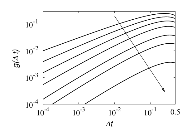
For any $H<1$ $g(\Delta t)>0$ for small $\Delta t$ , corresponding to the occurrence of tunneling. Conversely, for $H=1$ , i.e., for stochastic processes possessing a.e. smooth trajectories, $g(\Delta t)=0$ identically, and tunneling is completely hindered. This is the case of Poisson-Kac processes, and this simple argument supports the statement that trajectory regularity and the boundedness of the velocity (corresponding to the fact that $|r(t)|$ in eq. (80) admits an upper bound) are the two conditions preventing tunneling effects.

Therefore, tunneling barriers, controlling e.g. the occurrence of multiple stationary invariant densities in Poisson-Kac model, as discussed in [51], are the consequence of trajectory regularity which, in turn, is implied by the finite propagation velocity of these stochastic perturbations.

This observation opens up interesting observations in quantum mechanical problems: non-relativistic quantum-particles, obeying the Schrödinger equation, possess completely different tunneling properties of their relativistic counterpart obeying the Dirac equation (see e.g. the Klein paradox in the relativistic case) [79, 80]. Since the two quantum models, the non-relativistic Schrödinger, and the relativistic Dirac equations are related, via analytic continuation in the time variable, to Wiener and Poisson-Kac processes, respectively, it is not surprinsing, in the light of what above discussed, their completely different tunneling behaviors, which ultimately can be predicted from their stochastic counterparts. The case of tunneling is probably the indicator of something more basic: the analogy Schrödinger/Wiener processes vs Dirac/Poisson-Kac fluctuations in connection with tunneling phenomena is just the first point of attack in order to unveil the deep connections between stochastic fluctuations and quantum world at a fundamental physical level, i.e., beyond the simple mathematical claim that a purely formal analogy exists between these processes. We hope to analyze this issue in future works.

8 Concluding remarks

Starting from the analysis of some basic properties (Markovian nature, regularity of the trajectories), we have derived some general results for Poisson-Kac and GPK processes.

The extended Markovian nature and the notion of stochastic completeness can be viewed as two faces of the same coin. If information on the stochastic heat bath, perturbing the system, in retained in the statistical description, it is rather intuitive to expect that the Markovian nature of the process cannot be expressed as a strict Markovian condition involving solely the probability density function $p({\bf x},t)$ , but it should be stated in an extended form using a vector-valued system of partial probability densities. This is the case of GPK processes. The description involves a finite number $N$ of partial probability densities, just because the underlying stochastic process (the $N$ -state finite Poisson process) attains solely a finite number of states. As discussed in [54], if this description is generalized to an infinite number of states, then the corresponding complete stochastic description of the process involves a infinite-dimensional vector of partial probabilities.

The other relevant issue, thoroughly addressed in the article, is the almost everywhere regularity of the trajectories of GPK processes. The smoothness of the trajectories influences the thermodynamic formalism, as it permits to define the notion of local power (time derivative of work) delivered by the heat bath to the system.

It influences deeply the long-term qualitative properties. In Section 7, this qualitative difference between a Poisson-Kac process and a similar process driven by colored Wiener fluctuations has been connected to the compactness of the support of the unique stationary density function. Using other classes of deterministic biasing fields - different from a pure elastic force - this difference can be related to striking qualitative differences, such as ergodicity-breaking and the occurrence of multiple stationary invariant densities, as discussed thoroughly in [51], enforcing a deterministic bias giving rise to boundary-layer polarization.

As discussed in Section 7, the compactness of the stationary probability density in the Poisson-Kac processes is one-to-one with the tunneling capabilities of these stochastic systems which, in turn, is related essentially to trajectory regularity and not on the colored nature (correlation properties) of these stochastic perturbations (which is also a by-product of trajectory regularity).

The quantum implications of this result, especially as regards the relativistic case (the Dirac equation) will be addressed elsewhere. In point of fact, the relativistic implications of Poisson-Kac and GPK process are essentially based on their trajectory regularity, i.e., on the fact that their velocities are intrinsically bounded, which is the fundamental physical requirement imposed by the constant value of light velocity in vacuo. The use of Poisson-Kac processes in relativistic applications will be addressed in future works. This is a very delicate issue involving the meaning of stochastic fluctuations in relativistic systems and field theories.

References

[1] Öttinger H C 1996 Stochastic Processes in Polymeric Fluids (Springer Verlag, Berlin).
[2] Van Kampen N G 1992 Stochastic Processes in Physics and Chemistry (Elsevier, Amsterdam).
[3] Yuan R and Ao P 2012 Beyond Ito versus Stratonovich, J. Stat. Mech. 7 P07010 1-14.
[4] Moon W and Wettlaufer J S 2014 On the interpretation of Stratonovich calculus New J. Phys. 16 055017 1-13.
[5] Wong E and Zakai M 1965 On the convergence of ordinary integrals to stochastic integrals Ann. Math. Stat. 36 1560-1564.
[6] Twardowska K 1996 Wong-Zakai Approximations for Stochastic Differential Equations Acta Applicandae Mathematicae 43 317-359.
[7] Sekimoto K 2010 Stochastic Energetics (Springer-Verlag, Berlin).
[8] Klimontovich Yu. L. 1990 Ito, Stratonovich and Kinetic Forms of Stochastic Equations Physica A 165 515-532.
[9] Dunkel J and Hänggi P 2009 Relativistic Brownian motion Phys. Rep. 471 1-73.
[10] Li T and Raizen M G 2013 Brownian motion at short time scales Ann. Phys. (Berlin) 525 281-293.
[11] Kheifets S, Simha A, Melin K, Li T. and Raizen M G 2014 Observation of Brownian motion in liquids at short times: instantaneous velocity and memory loss Science 343 1493-1496.
[12] Krausz F and Ivanov M 2009 Attosecond physics Rev. Mod. Phys. 81 163-234.
[13] Fann W S, Storz R, Tom H W K and Bokor J 1992 Direct Measurement of Nonequilibrium Electron-Energy Distributions in Subpicosecond Laser-Heated Gold Films Phys. Rev. Lett. 68 2834-2837.
[14] Marciak-Kozlowska J, Mucha Z and Kozlowski M 1995 Picosecond Thermal Pulses in Thin Gold Films Int. J. Thermophysics 16 1489-1497.
[15] Seifert U 2012 Stochastic thermodynamics, fluctuation theorems and molecular machines Rep. Prog. Phys. 75 126001 1-58.
[16] Klages R, Just W and Jarzinski C (Eds.) 2013 Nonequilibrium Statistical Physics of Small Systems (Wiley-VCH, Weinheim).
[17] Garcia-Colin L S, Lopez de Haro M, Rodriguez R F, Casas-Vazquez J, Jou D 1984 On the Foundations of Extended Irreversible Thermodynamics J. Stat. Phys. 37 465-484.
[18] Jou D, Casas-Vazquez J and Lebon G 1988 Extended Irreversible Thermodynamics Rep. Prog. Phys. 51 1105-1179.
[19] Jou D, Casas-Vazquez J and Lebon G 1992 Extended irreversible thermodynamics: An overview of recent bibliography Non-Equilibrium Thermodynamics 17 383-396.
[20] Kac M 1974 A stochastic model related to the telegrapher’s equation Rocky Mountain J. Math. 4 497-509.
[21] Giona M Brasiello A and Crescitelli S 2016 Generalized Poisson–Kac Processes: Basic Properties and Implications in Extended Thermodynamics and Transport, J. Non-Equil. Thermodyn. 41 107-114.
[22] Cattaneo C 1958 On a form of heat equation which eliminates the paradox of instantaneous propagation C. R. Acad. Sci. Paris 247 431-433.
[23] Horsthemke W and Lefevre R 2006 Noise-Induced Transitions (Springer-Verlag, Berlin).
[24] Masoliver J 1992 Second-order processes driven by dichotomous noise Phys. Rev. A 45 706-713.
[25] Weiss G.H. 2002 Some applications of persistent random walks and the telegrapher’s equation Physica A 311 381-410.
[26] Gitterman 2003 Harmonic oscillator with multiplicative noise: Non-monotonic dependence on the strength and the rate of the dichotomous noise Phys. Rev. E 67 057103 1-4.
[27] Bena I 2006 Dichotomous Markov noise: exact results for out-of-equilibrium systems Int. J. Mod. Phys. B 20 2825-2888.
[28] Fiasconaro A, Spagnolo B, Ochab-Marcinek A and Gudowska-Nowak E 2006 Co-occurrence of resonant activation and noise-enhanced stability in a model of cancer growth in the presence of immune response Phys. Rev. E 041904 1-10.
[29] Kolesnik A D. and Ratanov N 2013 Telegraph Processes and Option Pricing (Springer-Verlag, Berlin).
[30] Plyukhin A V 2010 Stochastic process leading to wave equations in dimensios higher than one Phys. Rev. E 81 021113 1-5.
[31] Kolesnik A D and Turbin A F 1998 The equation of symmetric Markovian random evolution in a plane Stoch. Proc. Appl. 75 67-87.
[32] Kolesnik A. D. 2001 Weak Convergence of a Planar Random Evolution to the Wiener Process J. Theor. Prob. 14 485-494.
[33] Kolesnik A D 2008 Random Motions at Finite Speed in Higher Dimensions J. Stat. Phys. 131 1039-1065.
[34] Kolesnik A D and Pinsky M A 2011 Random Evolutions Are Driven by the Hyperparabolic Operators J. Stat. Phys. 142 828-846.
[35] Gaveau B, Jacobson T, Kac M and Schulman L S 1984, Relativistic Extension of the Analogy between Quantum Mechanics and Brownian Motion Phys. Rev. Lett. 53 419-422.
[36] McKeon D G C and Ord G N 1992 Time Reversal in Stochastic Processes and the Dirac Equation PPhys. Rev. Lett. 69 3-4.
[37] Kudo T and Ohba I 2002 Derivation of relativistic wave equation from the Poisson process Pramana 9 413-416.
[38] Balakrishnan V and Lakshmibala S 2005 On the connection between biased dichotomous diffusion and the one-dimensional Dirac equation New J. Phys. 7 11 1-11.
[39] Janssen A 1990 The Distance Between the Kac Process and the Wiener Process with Applications to Generalized Telegraph Equations J. Theor. Prob. 3 349-360.
[40] Marshall T W 1963 Random Electrodynamics Proc. R. Soc. Lond. A 276 475-491.
[41] Sakharov A D 1967 Vacuum quantum fluctuations in curved space and the theory of gravitation Dokl. Akad. Nauk SSSR 177 70-71.
[42] Boyer T H 1975 Random electrodynamics: The theory of classical electrodynamics with classical electromagnetic zero-point radiation Phys. Rev. D 11 790-808.
[43] Milonni P W and Barut A O 1980 (Eds.) Foundations of Radiation Theory and Quantum Electrodynamics (Springer-Verlag, New York).
[44] Müller I and Ruggeri T 1991 Extended Thermodynamics (Spinger Verlag, New York).
[45] Jou D, Casas-Vazquez J and Lebon G 2001 Extended Irreversible Themrodynamics (Springer-Verlag, Berlin).
[46] Jou D, Casas-Vazquez J and Lebon 1999 Extended thermodynamics revisited (1988-1998) Rep. Prog. Phys. 62 1035-1142.
[47] De Groot S R and Mazur P 1984 Non-Equilibrium Thermodynamics (Dover Publ., New York).
[48] Grad H 1949 On the kinetic theory of rarefied gases Comm. pure and applied Math. 2 331-407.
[49] Körner C and Bergmann H W 1998 The physical defects of the hyperbolic heat conduction equation Appl. Phys. A 67 397-401.
[50] Brasiello A, Crescitelli S and Giona M 2016 One-dimensional hyperbolic transport: positivity and admissible boundary conditions derived from the wave formulation Physica A 449 176-191.
[51] Giona M, Brasiello A and Crescitelli S 2016 Ergodicity-breaking bifurcations and tunneling in hyperbolic transport models Europhys. Lett. 112 30001 1-6.
[52] Giona M, Brasiello A and Crescitelli S 2016 On the influence of reflective boundary conditions on the statistics of Poisson–Kac diffusion processes Physica A 148-164.
[53] Giona M, Brasiello A and Crescitelli S 2016 Energetics of Poisson–Kac Stochastic Processes Possessing Finite Propagation Velocity J. Non-Equil. Thermodyn. 41 115-122.
[54] Giona M, Brasiello A and Crescitelli S 2016 Stochastic foundations of ondulatory transport phenomena: Generalized Poisson Kac processes I - Basic theory J. Phys A (submitted).
[55] Hänggi and Talkner P 1985 First-passage time problems for non-Markovian processes Phys. Rev. A 32 1934-1937.
[56] Luczka J, Hänggi P, Gadomski A 1995 Non-Markovian process driven by quadratic noise: Kramers-Moyal expansion and Fokker-Planck modelling Phys. Rev. E 51 2933-2938.
[57] Kitahara K, Horsthemke W, Lefevre R and Inaba Y 1980 Phase Diagrams of Noise Induced Transitions Prog. Theor. Phys. 64 1233-1247.
[58] Siegle P, Goychuk I, Talkner P and Hänggi P 2010 Markovian embedding of non-Markovian superdiffusion Phys. Rev: E 81 011136 1-10.
[59] Rabiner L R 1989 A tutorial on hidden Markov models and selected applications in speech recognition Proc. IEEE 77 257-286.
[60] Mohamed M A. and Gader P 2000 Generalized Hidden markov Models - Part I: Theoretical Frameworks IEEE Trans. Fuzzy Systems 8 67-81.
[61] Guckenheimer J and Holmes P 1983 Nonlinear oscillations, dynamical systems, and bifurcations of vector fields (Springer-Verlag, Berlin).
[62] Takens F 1980 Detecting strange attractors in turbulence in Dynamical Systems and Turbulence, Rand D and Young L.-S. (Eds.) pp. 366-381 (Springer-Verlag, Berlin).
[63] Rodriguez M A and Pesquera L 1986 First-passage times for non-Markovian processes driven by dichotomous Markov noise Phys. Rev. A 34 4532-4534.
[64] Weiss G H, Masoliver J, Lindenberg K and West B J 1987 First-passage times for non-Markovian processes: Multivalued noise Phys. Rev. A 36 1435-1439.
[65] Hernandez-Garcia H, Pesquera L, Rodriguez M A and San Miguel M 1987 First-passage time statistics: Processes driven by Poisson noise Phys. Rev. A 36 5774-5781.
[66] Balakrishnan V, Van den Broeck C and Hänggi P 1988 First-passage times of non-Markovian processes: The case of reflecting boundaries Phys. Rev. A 38 4213-4222.
[67] Pawula R F, Porrà J M and Masoliver J 1993 Mean first-passage times for systems driven by gamma and McFadden dichotomous noise Phys. Rev. E 47 189-201.
[68] Olarrea J, Parrondo J M R and de la Rubia F J 1995 Escape Statistics for Systems Driven by Dichotomous Noise I. General Theory J. Stat. Phys. 79 669-682.
[69] Olarrea J, Parrondo J M R and de la Rubia F J 1995 Escape Statistics for Systems Driven by Dichotomous Noise II. The Imperfect Pitchfork Bifurcation as a Case Study J. Stat. Phys. 79 683-699.
[70] Falconer K 1990 Fractal Geometry - Mathematical Foundations and Applications (J Wiley & Sons, Chichester).
[71] Meakin P Fractals 1998 Scaling and Growth Far from Equilibrium (Cambridge Univ. Press, Cambridge).
[72] Havlin S and Ben-Avraham D 1987 Diffusion in disordered media Adv. Phys. 36 695-798.
[73] Ben-Avraham D and Havlin S 2000 Diffusion and reactions in fractals and disordered media (Cambridge Univ. Press, Cambridge).
[74] Tricot C 1993 Curves and Fractal Dimension (Springer-Verlag, Berlin).
[75] Zwanzig R 1973 Nonlinear Generalized Langevin Equations J. Stat. Phys. 9 215-220.
[76] Hänggi P 1997 Generalized Langevin equations: A Useful Tool for the Perplexed Modeller of Nonequilibrium Fluctuations?, in Schimansky-Geier L. and Pöschel T. (Eds.) Stochastic Dynamics (Springer-Verlag, Berlin). pp. 15-22
[77] Arnold L, Horsthemke W and Lefevre R 1978 White and Coloured External Noise and Transition Phenomena in Nonlinear Systems Z. Physik B 29 367-373.
[78] Hänggi P and Jung P 1995 Colored noise in dynamical systems Adv. Chem. Phys. 89 239-326.
[79] Dombey N and Calogeracos 1999 Seventy years of the Klein paradox, Phys. Rep. 315 41-58.
[80] Robinson T R 2012 On Klein tunneling in graphene Am. J. Phys. 80 141-147.