Low Frequency Carbon Radio Recombination Lines I: Calculations of Departure Coefficients
Abstract
In the first paper of this series, we study the level population problem of recombining carbon ions. We focus our study on high quantum numbers anticipating observations of Carbon Radio Recombination Lines to be carried out by the LOw Frequency ARray (LOFAR). We solve the level population equation including angular momentum levels with updated collision rates up to high principal quantum numbers. We derive departure coefficients by solving the level population equation in the hydrogenic approximation and including low temperature dielectronic recombination effects. Our results in the hydrogenic approximation agree well with those of previous works. When comparing our results including dielectronic recombination we find differences which we ascribe to updates in the atomic physics (e.g., collision rates) and to the approximate solution method of the statistical equilibrium equations adopted in previous studies. A comparison with observations is discussed in an accompanying article, as radiative transfer effects need to be considered.
I Introduction
The interplay of stars and their surrounding gas leads to the presence of distinct phases in the interstellar medium (ISM) of galaxies (e.g. Field et al. 22, McKee & Ostriker 44). Diffuse atomic clouds (the Cold Neutral Medium, CNM) have densities of about and temperatures of about , where atomic hydrogen is largely neutral but carbon is singly ionized by photons with energies between and . The warmer () and more tenuous () intercloud phase is heated and ionized by FUV and EUV photons escaping from HII regions [84], usually referred to as the Warm Neutral medium (WNM) and Warm Ionized Medium (WIM). The phases of the ISM are often globally considered to be in thermal equilibrium and in pressure balance [64, 15]. However, the observed large turbulent width and presence of gas at thermally unstable, intermediate temperatures attests to the importance of heating by kinetic energy input. In addition, the ISM also hosts molecular clouds, where hydrogen is in the form of and self-gravity plays an important role. All of these phases are directly tied to key questions on the origin and evolution of the ISM, including the energetics of the CNM, WNM and the WIM; the evolutionary relationship of atomic and molecular gas; the relationship of these ISM phases with newly formed stars; and the conversion of their radiative and kinetic power into thermal and turbulent energy of the ISM (e.g. Cox 15, Elmegreen & Scalo 19, Scalo & Elmegreen 65, McKee & Ostriker 45).
The neutral phases of the ISM have been studied using optical and UV observations of atomic lines. These observations can provide the physical conditions but are limited to pinpoint experiments towards bright background sources and are hampered by dust extinction [70]. At radio wavelengths, dust extinction is not important and observations of the 21 cm hyperfine transition of neutral atomic hydrogen have been used to study the neutral phases (e.g. Weaver & Williams 82, Kalberla et al. 36, Heiles & Troland 31). On a global scale, these observations have revealed the prevalence of the two phase structure in the interstellar medium of cold clouds embedded in a warm intercloud medium but they have also pointed out challenges to this theoretical view [41, 37]. It has been notoriously challenging to determine the physical characteristics (density, temperature) of the neutral structures in the ISM as separating the cold and warm components is challenging (e.g. Heiles & Troland 30). In this context, Carbon radio recombination lines (CRRLs) provide a promising tracer of the neutral phases of the ISM (e.g. Peters et al. 56, Oonk et al. 51).
Carbon has a lower ionization potential (11.2 eV) than hydrogen (13.6 eV) and can be ionized by radiation fields in regions where hydrogen is largely neutral. Recombination of carbon ions with electrons to high Rydberg states will lead to CRRLs in the sub-millimeter to decameter wavelength range. Carbon radio recombination lines have been observed in the interstellar medium of our Galaxy towards two types of clouds: diffuse clouds (e.g.: Konovalenko & Sodin 40, Erickson et al. 20, Roshi et al. 59, Stepkin et al. 71, Oonk et al. 50) and photodissociation regions (PDRs), the boundaries of HII regions and their parent molecular clouds (e.g.: Natta et al. 48, Wyrowski et al. 85, Quireza et al. 58). The first low frequency (26.1 MHz) carbon radio recombination line was detected in absorption towards the supernova remnant Cas A by Konovalenko & Sodin [39] (wrongly attributed to a hyperfine structure line of , Konovalenko & Sodin 40). This line corresponds to a transition occurring at high quantum levels (). Recently, Stepkin et al. [71] detected CRRLs in the range 25.5–26.5 MHz towards Cas A, corresponding to transitions involving levels as large as .
Observations of low frequency carbon recombination lines can be used to probe the physical properties of the diffuse interstellar medium. However, detailed modeling is required to interpret the observations. Watson et al. [81], Walmsley & Watson [80] showed that, at low temperatures (), electrons can recombine with carbon ions by simultaneously exciting the fine structure line, a process known as dielectronic recombination11 1 This process has been referred in the literature as dielectronic-like recombination or dielectronic capture by Watson et al. [81] to distinguish from the regular dielectronic recombination. Dielectronic capture refers to the capture of the electron in an excited -state accompanied by simultaneous excitation of the core electron to the excited state. The captured electron can either auto ionize, collisional transferred to another state, or radiatively decay. Strictly speaking, dielectronic recombination refers to dieclectronic capture followed by stabilization. However, throughout this article we will use the term dielectronic recombination to refer to the same process as is common in the astronomical literature.. Such recombination process occurs to high states, and can explain the behavior of the high CRRLs observed towards Cas A. Walmsley & Watson [80] modified the code from Brocklehurst & Salem [11] to include dielectronic recombination. Payne et al. [54] modified the code to consider transitions up to 10000 levels. All of these results assume a statistical distribution of the angular momentum levels, an assumption that is not valid at intermediate levels for low temperatures. Moreover, the lower the temperature, the higher the -level for which that assumption is not valid.
The increased sensitivity, spatial resolution, and bandwidth of the Low Frequency ARray (LOFAR, van Haarlem et al. 77) is opening the low frequency sky to systematic studies of high quantum number radio recombination lines. The recent detection of high level carbon radio recombination lines using LOFAR towards the line of sight of Cas A [3], Cyg A [50], and the first extragalactic detection in the starburst galaxy M82 [47] illustrate the potential of LOFAR for such studies. Moreover, pilot studies have demonstrated that surveys of low frequency radio recombination lines of the galactic plane are within reach, providing a new and powerful probe of the diffuse interstellar medium. These new observations have motivated us to reassess some of the approximations made by previous works and to expand the range of applicability of recombination line theory in terms of physical parameters. In addition, increased computer power allows us to solve the level population problem considering a much larger number of levels than ever before. Furthermore, updated collisional rates are now available [79], allowing us to explicitly consider the level population of quantum angular momentum sub-levels to high principal quantum number levels. Finally, it can be expected that the Square Kilometer Array, SKA, will further revolutionize our understanding of the low frequency universe with even higher sensitivity and angular resolution [51].
In this work, we present the method to calculate the level population of recombining ions and provide some exemplary results applicable to low temperature diffuse clouds in the ISM. In an accompanying article (Salgado et al. 63, from here on Paper II), we will present results specifically geared towards radio recombination line studies of the diffuse interstellar medium. In Section II, we introduce the problem of level populations of atoms and the methods to solve this problem for hydrogen and hydrogenic carbon atoms. We also present the rates used in this work to solve the level population problem. In Section III, we discuss our results focusing on hydrogen and carbon atoms. We compare our results in terms of the departure coefficients with previous results from the literature. In Section IV, we summarize our results and provide the conclusions of the present work.
II Theory
A large fraction of our understanding of the physical processes in the Universe comes from observations of atomic lines in astrophysical plasmas. In order to interpret the observations, accurate models for the level population of atoms are needed as the strength (or depth) of an emission (absorption) line depends on the level populations of atoms. Here, we summarize the basic ingredients needed to build level population models and provide a basic description of the level population problem. We begin our discussion by describing the line emission and absorption coefficients ( and , respectively), which are given by [69, 26]:
| (1) | |||||
| (2) |
where is the Planck constant, is the level population of a given upper level () and is the level population of the lower level (); is the line profile, is the frequency of the transition and , are the Einstein coefficients for spontaneous and stimulated emission (absorption) 22 2 We provide the formulation to obtain the values for the rates in Appendix C., respectively.
Under local thermodynamic equilibrium (LTE) conditions, level populations are given by the Saha-Boltzmann equation (e.g. Brocklehurst 7):
| (3) |
where is the electron temperature, is the electron density in the nebula, is the ion density, is the electron mass, is the Boltzmann constant, is the Planck constant, is the speed of light and is the Rydberg constant; is the statistical weight of the level and angular quantum momentum level [, for hydrogen], and is the statistical weight of the parent ion. The factor is the thermal de Broglie wavelength, , of the free electron 33 3 .. In the most general case, lines are formed under non-LTE conditions and the level population equation must be solved in order to properly model the line properties as a function of quantum level ().
Following e.g. Seaton [66] and Brocklehurst [6], we present the results of our modeling in terms of the departure coefficients (), defined by:
| (4) |
and values are computed by taking the weighted sum of the values:
| (5) |
note that, at a given , the values for large levels influence the final value the most due to the statistical weight factor. At low frequencies stimulated emission is important [25] and we introduce the correction factor for stimulated emission as defined by Brocklehurst & Seaton [8]:
| (6) |
unless otherwise stated the presented here correspond to transitions (). The description of the level population in terms of departure coefficients is convenient as it reduces the level population problem to a more easily handled problem as we will show in Section II.1.
II.1 Level Population of Carbon Atoms under Non-LTE Conditions
The observations of high carbon recombination lines in the ISM motivated Watson et al. [81] to study the effect on the level population of dielectronic recombination and its inverse process (autoionization) in low temperature () gas. Watson et al. [81] used -changing collision rates 44 4 We use the term -changing collision rates to refer to collisions rate that induce a transition from state to from Jacobs & Davis [35] and concluded that for levels , dielectronic recombination of carbon ions can be of importance. In a later work, Walmsley & Watson [80] used collision rates from Dickinson [16] and estimated a value for which autoionization becomes more important than angular momentum changing rates. The change in collision rates led them to conclude that the influence of dielectronic recombination on the values is important at levels . Clearly, the results are sensitive to the choice of the angular momentum changing rates. Here, we will explicitly consider -sublevels when solving the level population equation.
The dielectronic recombination and autoionization processes affect only the C+ ions in the state, therefore we treat the level population for the two ion cores in the states separately in the evaluation of the level population [80]. The equations for carbon atoms recombining to the ion core population have to include terms describing dielectronic recombination () and autoionization (), viz.:
| (7) |
The left hand side of Equation 7 describes all the processes that take an electron out of the -level, and the right hand side the processes that add an electron to the level; is the coefficient for spontaneous emission, is the coefficient for stimulated emission or absorption induced by a radiation field ; is the coefficient for energy changing collisions (i.e. transitions with ), is the coefficient for -changing collisions; () is the coefficient for collisional ionization (3-body recombination) and is the coefficient for radiative recombination. A description of the coefficients entering in Equation 7 is given in Section II.3 and in further detail in the Appendix. The level population equation is solved by finding the values for the departure coefficients. The level population for carbon ions recombining to the level is hydrogenic and we solve for the departure coefficients () using Equation 7, but ignoring the coefficients for dielectronic recombination and autoionization.
After computing the and , we compute the departure coefficients ( and ) for both parent ion populations by summing over all -states (Equation 5). The final departure coefficients for carbon are obtained by computing the weighted average of both ion cores:
| (8) |
Note that, in order to obtain the final departure coefficients, the relative population of the parent ion cores is needed. Here, we assume that the population ratio of the two ion cores to is determined by collisions with electrons and hydrogen atoms. This ratio can be obtained using [57, 54]:
| (9) | |||||
| (10) |
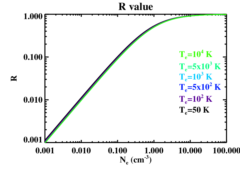
where is the de-excitation rate due to collisions with electrons, is the de-excitation rate due to collisions with hydrogen atoms [54] 55 5 Payne et al. [54] used rates from Tielens & Hollenbach [75], based on Launay & Roueff [42] for collisions with hydrogen atoms and Hayes & Nussbaumer [29] for collisions with electrons. Newer rates are available for collisions with electrons [83] and hydrogen atoms [5], but the difference in values is negligible., is the atomic hydrogen density and is the spontaneous radiative decay rate of the core. In this work, we have ignored collisions with molecular hydrogen, which should be included for high density PDRs. Collisional rates for H2 excitation of C+ have been calculated by Flower [23]. In the cases of interest here, the value of is dominated by collisions with atomic hydrogen. We recognize that the definition of given in Equation 9 is related to the critical density () of a two level system by where is the density of the collisional partner (electron or hydrogen). The LTE ratio of the ion core is given by the statistical weights of the levels and the temperature () of the gas:
| (11) |
where are the statistical weights of the fine structure levels and is the energy difference of the fine structure transition. The LTE level population ratio as a function of temperature is shown in Figure 1, illustrating the strong dependence on temperature of this value. At densities below the critical density ( for collisions with H), the fine structure levels fall out of LTE and the value for becomes very small (Figure 1). Note that is not very sensitive to the temperature.
With the definition of given above, the final departure coefficient can be written as [57]:
| (12) |
The final departure coefficient is the value that we are interested in to describe CRRLs.

II.2 Numerical Method
Having described how to derive the , now we focus on the problem of obtaining the departure coefficients for both ion cores from the level population equation. We use the same procedure to obtain the departure coefficients for both parent ion cores, as the only difference in the level population equation for the and the cores is the inclusion of dielectronic recombination and autoionization processes. We will refer as and without making a distinction between the and in this subsection.
We follow the methods described in Brocklehurst [7] and improved in Hummer & Storey [33] to solve the level population equation in an iterative manner. First, we solve the level population equation by assuming that the sublevels are in statistical equilibrium, i.e. for all sublevels. We refer to this approach as the -method (see Appendix B). Second, we used the previously computed values to determine the coefficients on the right hand side of Equation 7 that contain terms with . Thus, the level population equation for a given is a tridiagonal equation on the sublevels involving terms of the type . This tridiagonal equation is solved for the values (further details are given in Appendix B). The second step of this procedure is repeated until the difference between the computed departure coefficients is less than 1%.
We consider a fixed maximum number of levels, , equal to 9900. We make no explicit assumptions on the asymptotic behavior of the for larger values of . Therefore, no fitting or extrapolation is required for large . The adopted value for is large enough for the asymptotic limit – for – to hold even at the lowest densities considered here. For the -method, we need to consider all sublevels up to a high level (). For levels higher than this critical level (), we assume that the sublevels are in statistical equilibrium. In our calculations , regardless of the density.
II.3 Rates Used in this Work
In this section, we provide a brief description of the rates used in solving the level populations. Further details and the mathematical formulations for each rate are given in Appendices C, D, E and F. Accurate values for the rates are critical to obtain meaningful departure coefficients when solving the level population equation (Equation 7). Radiative rates are known to high accuracy () as they can be computed from first principles. On the other hand, collision rates at low temperatures are more uncertain (, Vriens & Smeets 78).
II.3.1 Einstein A and B coefficient
The Einstein coefficients for spontaneous and stimulated transitions can be derived from first principles. We used the recursion formula described in Storey & Hummer [73] to obtain the values for the Einstein coefficients. To solve the method (our first step in solving the level population equation) we require the values for , which can be easily obtained by summing the :
| (13) |
The mathematical formulation to obtain values for spontaneous transitions is detailed in Appendix C.
The coefficients for stimulated emission and absorption () are related to the coefficients by:
| (14) | |||||
| (15) |
II.3.2 Energy changing collision rates
In general, energy changing collisions are dominated by the interactions of electrons with the atom. The interaction of an electron with an atom can induce transitions of the type:
| (16) |
with changing the distribution of electrons in an atom population. Hummer & Storey [33] used the formulation of Percival & Richards [55]. The collision rates derived by Percival & Richards [55] are essentially the same as Gee et al. [24]. However, the collision rates from Gee et al. [24] are not valid for the low temperatures of interest here. Instead, we use collision rates from Vriens & Smeets [78]. We note that at high and for high levels, the Bethe (Born) approximation holds and values of the rates from Vriens & Smeets [78] differ by less than 20% when compared to those from Gee et al. [24]. The good agreement between the two rates is expected since the results from Vriens & Smeets [78] are based on Gee et al. [24]. On the other hand, at low and for low levels values the two rates differ by several orders of magnitude and, indeed, the Gee et al. [24] values are too high to be physically realistic. A comparison of the rates for different values of and transitions is shown in Figure 2. We explore the effects of using Vriens & Smeets [78] rates on the values in Section III.2.
The inverse rates are obtained from detailed balance:
| (17) |
In order to solve the -method, rates of the type with are needed. Here, the approach of Hummer & Storey [33] is followed and the collision rates are normalized by the oscillator strength of the transitions (Equation 5 in Hummer & Storey 33). Only transitions with were included as these dominate the collision process [33],.


II.3.3 Angular momentum changing collision rates
For low levels, the level population has to be explicitly calculated. Moreover, for the dielectronic recombination process, the angular momentum changing collisions set the value for which the dielectronic recombination process is important, and transitions of the type:
| (18) |
must be considered. In general, collisions with ions are more important than collisions with electrons. Here, for simplicity, we adopt that is the dominant cation.
Hummer & Storey [33] used -changing collision rates from Pengelly & Seaton [28] which are computed iteratively for a given level starting at or . However, as pointed out by Hummer & Storey [33] and Brocklehurst [7], the values for the -changing rates obtained by starting the iterations at differ from those obtained when starting at . Moreover, averaging the -changing rates obtained by the two different initial conditions leads to an oscillatory behavior of the rates that depends on [6]. Hummer & Storey [33] circumvented this problem by normalizing the value of the rates by the oscillator strength (Equation 4 in Hummer & Storey 33). In addition, at high levels and high densities the values for can become negative (Equation 43 in Pengelly & Seaton 28). This poses a problem when studying the level population of carbon atoms at the high levels of interest in the present work66 6 We note that this was not a problem for Hummer & Storey [33], since they assumed an statistical distribution of the levels for high .. The more recent study of Vrinceanu et al. [79] provides a general formulation to obtain the value of -changing transition rates. These new rates use a much smaller cut-off radius of the probability of the transition for large impact parameters. Furthermore, the rates from Vrinceanu et al. [79] are well behaved over a large range of temperature and densities and they do not exhibit the oscillatory behavior with sublevel shown by the Pengelly & Seaton [28] rates. Therefore, we use the Vrinceanu et al. [79] rates in this work. Vrinceanu et al. [79] derived the following expression, valid for and :
| (19) |
where is the Bohr radius and is the reduced mass of the system. Values for the inverse process are obtained by using detailed balance:
| (20) |
We note that the -changing collision rates obtained by using the formula from Vrinceanu et al. [79] can differ by a factor of six [79] with those using the Pengelly & Seaton [28] formulation. We discuss the effect on the final values in Section III.2, where we compare our results with those of Storey & Hummer [74] in the Hydrogenic approximation and with those of Ponomarev & Sorochenko [57] for carbon atoms.
II.3.4 Radiative Recombination
Radiative ionization occurs when an excited atom absorbs a photon with enough energy to ionize the excited electron. The process can be represented as follows:
| (21) |
and the inverse process is radiative recombination. We use the recursion relation described in Storey & Hummer [73] to obtain values for the ionization cross-section (Appendix D). Values for the radiative recombination () coefficients were obtained using the Milne relation and standard formulas (e.g. Rybicki & Lightman [60], Appendix D). The program provided by Storey & Hummer [73] only produces reliable values up to due to cancellation effects in the iterative procedure. In order to avoid cancellation effects, the values computed here were obtained by working with logarithmic values in the recursion formula. As expected, our values for the rates match those of Storey & Hummer [73] well.
For the -method we require the sum of the individual values:
| (22) |
The averaged values agree well with the approximated formulation of Seaton [66] to better than 5%, validating our approach.
II.3.5 Collisional ionization and 3-body recombination
Collisional ionization occurs when an atom encounters an electron and, due to the interaction, a bound electron from the atom is ionized. Schematically the process can be represented as:
| (23) |
The inverse process is given by the 3-body recombination and the value for the 3-body recombination rate is obtained from detailed balance:
| (24) | |||||
We used the formulation of Brocklehurst & Salem [11] and compared the values with those from the formulation given by Vriens & Smeets [78]. For levels above 100 and at , the Brocklehurst & Salem values are a factor of larger, but the differences quickly decrease for higher temperatures. To obtain the that are needed in the -method, we followed Hummer & Storey [33] and assumed that the rates are independent of the angular momentum. The mathematical formulation is reproduced in the Appendix F for convenience of the reader.
II.3.6 Dielectronic Recombination and Autoionization on Carbon Atoms
The dielectronic recombination process involves an electron recombining into a level while simultaneously exciting one of the bound electrons (left side of Equation 25, below). This state () is known as an autoionizing state. In this autoionizing state, the atom can stabilize either by releasing the recombined electron through autoionization (inverse process of dielectronic recombination) or through radiative stabilization (right hand side of Equation 25). Dielectronic recombination and autoionization are only relevant for atoms with more than one electron.
| (25) |
For C+ recombination, at free electrons in the plasma can recombine to a high level, and the kinetic energy is transfered to the core of the ion, producing an excitation of the fine-structure level of the C+ atom core (which has a difference in energy ). Due to the long radiative lifetime of the fine-structure transition (), radiative stabilization can be neglected.
Following Watson et al. [81], Ponomarev & Sorochenko [57], who compute the autoionization rate using the formulation by Seaton & Storey [68], i. e. :
| (26) |
with the collision strength for the excitation at the threshold. As Watson et al. [81], we used the formula obtained by Osterbrock [53]:
| (27) |
valid for . In order to avoid the singularity at we computed the autoionization rate, , from the approximate expression given in Dickinson [16]:
| (28) |
which is valid for . The dielectronic recombination rate is obtained by detailed balance:
| (29) |
Walmsley & Watson [80] defined as the departure coefficient when autoionization/dielectronic recombination dominate:
| (30) | |||||
A comparison of the dielectronic recombination rate with values from the literature is hampered by the focus of previous works on higher temperatures. The calculations of dielectronic recombination rates for Carbon from Nussbaumer & Storey [49] did not include fine structure transitions and are not suited for a direct comparison with the study presented here. Furthermore, the values presented by Gu [27] are given for higher temperatures than those studied here. The more recent study of Altun et al. [2] provides state resolved values for dielectronic recombination rates. For the physical conditions of interest in this article and for the fine structure levels of interest here, Altun et al. [2] provides values using intermediate coupling. However, a direct comparison with the results from Altun et al. [2] is not possible since they only include type dielectronic recombination resonances associated with the excitation of a electron to a level (see Equation 1 in Altun et al. 2).
III Results
The behavior of CRRLs with frequency depends on the level population of carbon via the departure coefficients. We compute departure coefficients for carbon atoms by solving the level population equation using the rates described in Section II.3 and the approach in Section II.2. Here, we present values for the departure coefficients and provide a comparison with earlier studies in order to illustrate the effect of our improved rates and numerical approach. A detailed analysis of the line strength under different physical conditions relevant for the diffuse clouds and the effects of radiative transfer are provided in an accompanying article (Paper II).
III.1 Departure Coefficient for Carbon Atoms
The final departure coefficients for carbon atoms (i.e. ) are obtained by computing the departure coefficients recombining from both parent ions, those in the level and those in the level. Therefore, it is illustrative to study the individual departure coefficients for the core, which are hydrogenic, and the departure coefficients for the core separately.
III.1.1 Departure Coefficient in the Hydrogenic Approximation
In Figure 3 we show example and values obtained in the hydrogenic approximation at for a large range in density. The behavior of the values as a function of can be understood in terms of the rates that are included in the level population equation. At the highest levels, collisional ionization and three body recombination dominate the rates in the level population equation and the values are close to unity. We can see that as the density increases, collisional equilibrium occurs at lower levels and the values approach unity at lower levels. In contrast, for the lowest levels, the level population equation is dominated by radiative processes and the levels drop out of collisional equilibrium. As the radiative rates increase with decreasing level, the departure coefficients become smaller. We note that differences in the departure coefficients for the low levels for different temperatures are due to the radiative recombination rate, which has a dependence.
At intermediate levels, the behavior of the as a function of shows a more complex pattern with a pronounced “bump” in the values for intermediate levels (). To guide the discussion we refer the reader to Figure 3. Starting at the highest , , as mentioned above. For these high levels, -changing collisions efficiently redistribute the electron population among the states and, at high density, the departure coefficients are unity as well (Figure 4, upper panels). For lower values of , the values decrease due to an increased importance of spontaneous transitions. At these levels, the values obtained by the method differ little from the values obtained by the -method, since -changing collisions efficiently redistribute the electrons among the sublevels for a given level. For lower levels, the effects of considering the sublevel distribution become important as -changing collisions compete with spontaneous decay, effectively “storing” electrons in high sublevels for which radiative decay is less important. collisions compete with spontaneous decay, effectively “storing” electrons in high sublevels for which radiative decay is less important. Specifically, the spontaneous rate out of a given level is approximately , and is higher for lower sublevels. Thus, high- sublevels are depopulated more slowly relative to lower sublevels on the same level. This results in a slight increase in the departure coefficients. Reflecting the statistical weight factor in Equation 5, the higher sublevels dominate the final value resulting in an increase in the final value. As the density increases, the sublevels approach statistical distribution faster. As a result, the influence of the sublevel population on the final is larger for lower densities than for higher densities at a given . The interplay of the rates produce the “bump” which is apparent in the distribution (Figure 3)
The influence of -changing collisions on the level populations and the resulting increase in the values was already presented by Hummer & Storey [33] and analyzed in detail by Strelnitski et al. [72] in the context of hydrogen masers. The results of our level population models are in good agreement with those provided by Hummer & Storey [33] as we show in Section III.2.


III.1.2 Departure Coefficient for Carbon Atoms Including Dielectronic Recombination
Only carbon atoms recombining to the ion core are affected by dielectronic recombination. Having analyzed the departure coefficients for the hydrogenic case, we focus now on the values and the resulting as introduced in Section II.1.
Figure 5 show example values for for and electron densities between . As pointed out by Watson et al. [81], the low lying sublevels are dominated by the dielectronic process and the values are equal to (Equation 30). As can be seen in Figure 1, such values can be much larger than unity at low densities resulting in an overpopulation of the low levels for the ion cores. In Figure 6 we show as a function of level under the same conditions. We see that at high electron densities the departure coefficients show a similar behavior as the hydrogenic values. Furthermore, an increase in the level population to values larger than unity is seen at low densities and moderate to high temperatures.
To guide the discussion, we analyze the behavior of the when autoionization/dielectronic recombination dominates. This occurs at different levels depending on the values of and considered. Nevertheless, it is instructive to understand the behavior of the level population in extreme cases. When autoionization/dielectronic recombination dominate, the in Equation 12 is given by:
| (31) |
At high densities, approaches unity and we note two cases. The first case is when is high, the maximum value of , meaning that a large fraction of the ions are in the core. Consequently, , thus the effect of dielectronic recombination is to increase the level population as compared to the hydrogenic case. We also note that since the final . The second case we analyze is for low , where the ion LTE ratio is low and most of the ions are in the core. Thus, and the departure coefficients are close to hydrogenic.
At low densities, and, as above, we study two cases. The first is when is high, the maximum value of and , therefore dielectronic recombination produces a large overpopulation as compared to the hydrogenic case. The second case is when is low and most of the ions are in the level and, as in the high density case, the . We note from this analysis that overpopulation of the (relative to the hydrogenic case) is only possible for a range of temperatures and densities. In particular, is maximum for high temperatures and low densities.
Having analyzed the behavior of the values in the extreme case, now we analyze the behavior of with . The population in the low levels is dominated by dielectronic recombination [81, 80] and up until a certain level where begins to decrease down to a value of one. The value where this change happens depends on temperature, moving to higher levels as decreases. To understand this further, we analyze the rates involved in the sublevel population (Figure 5). The low sublevels are dominated by dielectronic recombination and autoionization and the values for the ion cores are . For the higher sublevels other processes (mainly collisions) populate or depopulate electrons from the level and the net rate is lower than that of the low dielectronic recombination/autoionization. This lowers the value, which is effectively delayed by -changing collisions since they redistribute the population of electrons in the level. The for highest values dominate the value of due to the statistical weight factor.
We note that the behavior of the cores as a function of (see Figure 7) can be approximated by:
| (32) |
with defined as in Walmsley & Watson [80] (Equation 30) and was derived from fitting our results:
| (33) |
In diffuse clouds the integrated line to continuum ratio is proportional to . We note that the behavior is more complex as can be seen in Figure 8. The low “bump” on the makes the high at low densities and for levels between about and . Since the values decrease from values larger than one to approximately one, the changes sign. In Figure 9 we show the electron density as a function of the level where the change of sign on the occurs. At temperatures higher than about , our models for show no change of sign due to the combined effects of -changing collisions and dielectronic recombination.


III.2 Comparison with Previous Models
The level population of hydrogenic atoms is a well studied problem. Here, we will describe the effects of the updated collision rates as well as point out differences due to the improved numerical method.
III.2.1 Hydrogenic Atoms
At the lowest densities, we can compare our results for hydrogenic atoms with the values of Martin [43] for Hydrogen atoms. The results of Martin [43] were obtained in the low density limit, i.e. no collision processes were taken into account in his computations. The results are given in terms of the emissivity of the line normalized by the H emissivity. As can be seen in Figure 10, our results agree to better than 5%, and for most levels to better than 0.5%.
At high densities, we compare the hydrogenic results obtained here with those of Hummer & Storey [33]. Our approach reproduces well the (and ) values of Hummer & Storey [33] (to better than 1%) when using the same collision rates [24, 28] as can be seen in Figure 11. We note that the effect of using different energy changing rates () has virtually no effect on the final values. On the other hand, using Vrinceanu et al. [79] values for the rates results in differences in the values of 30% at . As expected, the difference is less at higher temperatures and densities since values are closer to equilibrium (see Figure 12). At low levels, our results for high levels are overpopulated as compared to the values of Hummer & Storey [33] leading to an increases in the values.


III.2.2 Carbon
Now we compare departure coefficients obtained here with the results of Ponomarev & Sorochenko [57] and the effect of including -changing collisions on the departure coefficients, see Figures 13 and 14. We will focus the discussion on the values from Ponomarev & Sorochenko [57] as the Walmsley & Watson [80] values are similar.
While the results presented here are remarkably different from those of Walmsley & Watson [80] and Ponomarev & Sorochenko [57], some trends are similar. We will first discuss the differences. Our results in Figures 13 and 14 show a pronounced ’bump’ for low in the range 50 to 150. This bump is similar to what we see for the hydrogenic approximation but enhanced by dielectronic recombination (c.f. Figures 3.6 and 8; Section 3.1.2). As discussed in Section 3.1.1 this bump arises at these intermediate levels because collisions compete with spontaneous decay, effectively ’storing’ electrons in high sublevels for which radiative decay is less important. This means that the inclusion of -changing collisions leads to significantly larger values for in the range 50 to 150 as compared to Ponomarev & Sorochenko [57]. Regardless of the -changing collision rates used, at higher we note that our values with increasing asymptotically approach unity much faster than Ponomarev & Sorochenko [57]. This is especially true for lower electron densities (1.0 cm-3) and a direct consequence of using the -method to compute the departure coefficients.
Although the detailed behavior of our values differs strongly from Ponomarev & Sorochenko [57] there are also similarities in the general trends that we observe as a function of electron density and temperature. In particular, the very low and very high asymptotic behavior of the values is similar to Ponomarev & Sorochenko [57] in that the highest electron densities for a given electron temperature have the lowest values at low and approach equilibrium (=1) the fastest with increasing . For higher electron densities and lower electron temperatures, our results become increasingly similar to the hydrogenic case and agree with Ponomarev & Sorochenko [57]. This is expected as, as discussed in Section 3.1 at high densities the values approach equilibrium.
In terms of our results show, as expected, good agreement with the hydrogenic case and Ponomarev & Sorochenko [57] in the high density and low temperature limit. However, for the lower densities and higher temperatures shown in Figures 13 and 14 our models predict values that are lower by up to about an order of magnitude as compared to Ponomarev & Sorochenko [57]. This is particularly striking for the =100 K and =0.05 cm-3 model shown in Figure 14 where we find that both the maximum negative value and maximum positive value are more than an order of magnitude lower than the corresponding Ponomarev & Sorochenko [57] values.
Since the integrated optical depth is directly proportional to the value of (e.g. Salgado et al. 63, Walmsley & Watson 80, Shaver 69) we can interpret as a stimulation factor. This means that, for a given set of physical conditions, our models predict much lower maximum integrated optical depths for Carbon as compared to earlier investigations (e.g. Walmsley & Watson 80, Ponomarev & Sorochenko 57). This is true for both emission (negative ) and absorption (positive ). In particular, our models predict that equilibrium will be reached at much lower (typically around ) and thus that the integrated optical at high (low frequencies) will show a rather flat behavior for 600 whereas the previous models by Walmsley & Watson [80] and Ponomarev & Sorochenko [57] predict a strong increase with increasing .
We find that although our values asymptotically approach equilibrium at high that this value is not yet reached at . Therefore, the values we find are nearly, but not yet completely, constant in the range 600-1000 and as such the dependence of integrated optical depth on remains important at high . Finally, we note that for sufficiently high electron temperatures and low electron densities our models predict the existence of a region at intermediate (100-200) where the values can become positive. This behavior is a direct consequence of the inclusion of -changing collisions in our models. A more detailed comparison of the departure coefficients obtained using the -changing collision from Pengelly & Seaton [28] and those using the rates from Vrinceanu et al. [79] (Figure 15) reveals differences of less than 30% for the conditions of interest for CRRL studies.
Apart from the -changing collisions there are other potentially important differences between our models and those published by Ponomarev & Sorochenko [57]. Ponomarev & Sorochenko [57] do not provide the explicit values of the dielectronic recombination rates that they use. However, they refer back to Walmsley & Watson [80] for these rates and as we use the same formalism, we do not think that the dielectronic recombination rates are at the heart of the discrepancy. may have influenced their results. In addition, we note that we use somewhat different collision rates in our simulations. However, as illustrated in Figure 13 and 14, the exact collision rates have only limited influence on the values. Rather, we suspect that the approximate way the statistical equilibrium equations are solved by Ponomarev & Sorochenko [57] may have influenced their results and that including -changing collisions properly rather than adopting a statistical populations as did Ponomarev & Sorochenko [57] is key.
A further assessment of the effect of any uncertainty in the adopted dielectronic recombination rates on the final departure coefficients can be performed by arbitrarily multiplying the dielectronic recombination rate by a factor. We note that a dielectronic recombination rate a factor of 30% higher (lower) increases (decreases) the departure coefficients at low levels () by 30%. At the higher levels of interest for the study of CRRLs, () a factor of 30% on the dielectronic recombination rates changes the values of the departure coefficients by less than 10% (Figure 16, upper panels). As expected, the values for are affected more by the change on the dielectronic recombination rate and can be altered by a factors of a few (Figure 16, lower panels). It is clear that quantitative interpretation of carbon radio recombination lines would be served by more accurate dielectronic recombination rates that include the fine structure levels.


IV Summary and Conclusions
We have solved the level population equation for hydrogenic atoms using novel rates involved in the process. The level population equation is solved in two approximations: the and the method. The departure coefficients obtained using the method are similar to values from the literature (e.g. Brocklehurst 6 and Shaver 69). Our results using the method reproduce those from Hummer & Storey [33] well, once allowance is made for updates in the collisional rates.
By including the dielectronic recombination process together with the method we are able to model the level population of carbon in terms of the departure coefficients. Our results are qualitatively similar to those of Watson et al. [81], Walmsley & Watson [80]. However, the values obtained here differ considerably from those from the literature. The differences can be understood in terms of the use of improved collision rates and the improved numerical approach using the method. We confirm that dielectronic recombination can indeed produce an increase on the values of the departure coefficients at high levels compared to the hydrogenic values.
In anticipation of low frequency radio recombination line surveys of the diffuse interstellar medium now being undertaken by LOFAR, we have expanded the range of applicability of the formulation to the conditions of the cold neutral medium. For this environment, external radiation fields also become important at intermediate principal quantum levels while at high levels the influence of radiation fields on the level population is less important In an accompanying paper [63], we discuss the expected line strength for low frequency carbon radio recombination lines and the influence of an external radiation field. Throughout this work we have used a zero radiation field. In this companion paper we compare our results to existing observations of CRRLs towards Cas A and regions in the inner galaxy. We also describe the analysis techniques and diagnostic diagrams that can be used to analyze the forthcoming LOFAR CRRL survey. The departure coefficients obtained here will be used to analyze the LOFAR observations of Cas A in a future article [52].
References
- [1] Allen, C. W. 1973, London: University of London, Athlone Press, —c1973, 3rd ed.
- [2] Altun, Z., Yumak, A., Badnell, N. R., Colgan, J., & Pindzola, M. S. 2004, A&A, 420, 775
- [3] Asgekar, A., Oonk, J. B. R., Yatawatta, S., et al. 2013, A&A, 551, LL11
- [4] Baker, J. G., & Menzel, D. H. 1938, ApJ, 88, 52
- [5] Barinovs, G., van Hemert, M.C., Krems, R., Dalgarno, A. 2005, ApJ, 620, 537
- [6] Brocklehurst, M. 1970, MNRAS, 148, 417
- [7] Brocklehurst, M. 1971, MNRAS, 153, 471
- [8] Brocklehurst, M., & Seaton, M. J. 1972, MNRAS, 157, 179
- [9] Brocklehurst, M. 1973, Astrophys. Lett., 14, 81
- [10] Brocklehurst, M., & Salem, M. 1975, Computer Physics Communications, 9, 258
- [11] Brocklehurst, M., & Salem, M. 1977, Computer Physics Communications, 13, 39
- [12] Burgess, A. 1958, MNRAS, 118, 477
- [13] Burgess, A. 1965, MmRAS, 69, 1
- [14] Burgess, A., & Percival, I. C. 1968, Advances in Atomic and Molecular Physics, 4, 109
- [15] Cox, D. P. 2005, ARA&A, 43, 337
- [16] Dickinson, A. S. 1981, A&A, 100, 302
- [17] Dupree, A. K. 1972, ApJ, 173, 293
- [18] Ellingson, S. W., Taylor, G. B., Craig, J., et al. 2013, IEEE Transactions on Antennas and Propagation, 61, 2540
- [19] Elmegreen, B. G., & Scalo, J. 2004, ARA&A, 42, 211
- [20] Erickson, W. C., McConnell, D., & Anantharamaiah, K. R. 1995, ApJ, 454, 125
- [21] Ferrière, K. M. 2001, Reviews of Modern Physics, 73, 1031
- [22] Field, G. B., Goldsmith, D. W., & Habing, H. J. 1969, ApJ, 155, L149
- [23] Flower, D.R. 1988, J Phys B, 21, L451
- [24] Gee, C. S., Percival, L. C., Lodge, J. G., & Richards, D. 1976, MNRAS, 175, 209
- [25] Goldberg, L. 1966, ApJ, 144, 1225
- [26] Gordon, M. A., & Sorochenko, R. L. 2009, Astrophysics and Space Science Library, 282,
- [27] Gu, M. F. 2003, ApJ, 590, 1131
- [28] Pengelly, R. M., & Seaton, M. J. 1964, MNRAS, 127, 165
- [29] Hayes, M. A., & Nussbaumer, H. 1984, A&A, 134, 193
- [30] Heiles, C., & Troland, T. H. 2003, ApJS, 145, 329
- [31] Heiles, C., & Troland, T. H. 2003, ApJ, 586, 1067
- [32] Hilborn, R. C. 1982, American Journal of Physics, 50, 982
- [33] Hummer, D. G., & Storey, P. J. 1987, MNRAS, 224, 801
- [34] Hummer, D. G., & Storey, P. J. 1992, MNRAS, 254, 277
- [35] Jacobs, V. L., & Davis, J. 1978, Phys. Rev. A, 18, 697
- [36] Kalberla, P. M. W., Burton, W. B., Hartmann, D., et al. 2005, A&A, 440, 775
- [37] Kalberla, P. M. W., & Kerp, J. 2009, ARA&A, 47, 27
- [38] Kantharia, N. G., Anantharamaiah, K. R., & Payne, H. E. 1998, ApJ, 506, 758
- [39] Konovalenko, A. A., & Sodin, L. G. 1980, Nature, 283, 360
- [40] Konovalenko, A. A., & Sodin, L. G. 1981, Nature, 294, 135
- [41] Kulkarni, S. R., & Heiles, C. 1987, Interstellar Processes, 134, 87
- [42] Launay, J.-M., & Roueff, E. 1977, Journal of Physics B Atomic Molecular Physics, 10, 879
- [43] Martin, P. G. 1988, ApJS, 66, 125
- [44] McKee, C. F., & Ostriker, J. P. 1977, ApJ, 218, 148
- [45] McKee, C. F., & Ostriker, E. C. 2007, ARA&A, 45, 565
- [46] Morabito, L. K., van Harten, G., Salgado, F., et al. 2014, MNRAS, 441, 2855
- [47] Morabito, L. K., Oonk, J. B. R., Salgado, F., et al. 2014, ApJ, 795, LL33
- [48] Natta, A., Walmsley, C. M., & Tielens, A. G. G. M. 1994, ApJ, 428, 209
- [49] Nussbaumer, H., & Storey, P. J. 1983, A&A, 126, 75
- [50] Oonk, J. B. R., van Weeren, R. J., Salgado, F., et al. 2014, MNRAS, 437, 3506
- [51] Oonk, J. B. R., Morabito, L. K., Salgado, F., et al. 2015a, arXiv:1501.01179
- [52] Oonk, J. B. R., et al, in preparation
- [53] Osterbrock, D. E. 1965, ApJ, 142, 1423
- [54] Payne, H. E., Anantharamaiah, K. R., & Erickson, W. C. 1994, ApJ, 430, 690
- [55] Percival, I. C., & Richards, D. 1978, MNRAS, 183, 329
- [56] Peters, W. M., Lazio, T. J. W., Clarke, T. E., Erickson, W. C., & Kassim, N. E. 2011, A&A, 525, A128
- [57] Ponomarev, V. O., & Sorochenko, R. L. 1992, Soviet Astronomy Letters, 18, 215
- [58] Quireza, C., Rood, R. T., Balser, D. S., & Bania, T. M. 2006, ApJS, 165, 338
- [59] Roshi, D. A., Kantharia, N. G., & Anantharamaiah, K. R. 2002, A&A, 391, 1097
- [60] Rybicki, G. B., & Lightman, A. P. 1986, Radiative Processes in Astrophysics, by George B. Rybicki, Alan P. Lightman, pp. 400. ISBN 0-471-82759-2. Wiley-VCH , June 1986.,
- [61] Salem, M. 1975, MNRAS, 173, 513
- [62] Salem, M., & Brocklehurst, M. 1979, ApJS, 39, 633
- [63] Salgado, F., et al. accepted (Paper II)
- [64] Savage, B. D., & Sembach, K. R. 1996, ARA&A, 34, 279
- [65] Scalo, J., & Elmegreen, B. G. 2004, ARA&A, 42, 275
- [66] Seaton, J. M 1959, MNRAS, 119, 81
- [67] Seaton, J. M 1959, MNRAS, 119, 90
- [68] Seaton, M. J., & Storey, P. J. 1976, Atomic processes and applications. P. G. Burke (ed.), North-Holland Publ. Co., Amsterdam, Netherlands, p. 133 - 197, 133
- [69] Shaver, P. A. 1975, Pramana, 5, 1
- [70] Snow, T. P., & McCall, B. J. 2006, ARA&A, 44, 367
- [71] Stepkin, S. V., Konovalenko, A. A., Kantharia, N. G., & Udaya Shankar, N. 2007, MNRAS, 374, 852
- [72] Strelnitski, V. S., Ponomarev, V. O., & Smith, H. A. 1996, ApJ, 470, 1118
- [73] Storey, P. J., & Hummer, D. G. 1991, Computer Physics Communications, 66, 129
- [74] Storey, P. J., & Hummer, D. G. 1995, MNRAS, 272, 41
- [75] Tielens, A. G. G. M., & Hollenbach, D. 1985, ApJ, 291, 722
- [76] Tingay S. J., Goeke R., Bowman, J. D., et al. 2013, PASA, 30, 7
- [77] van Haarlem M. P., Wise M. W., Gunst A. W., et al. 2013, A&A, 556, 2
- [78] Vriens, L., & Smeets, A. H. M. 1980, Phys. Rev. A, 22, 940
- [79] Vrinceanu, D., Onofrio, R., & Sadeghpour, H. R. 2012, ApJ, 747, 56
- [80] Walmsley, C. M., & Watson, W. D. 1982, ApJ, 260, 317
- [81] Watson, W. D., Western, L. R., & Christensen, R. B. 1980, ApJ, 240, 956
- [82] Weaver, H., & Williams, D. R. W. 1973, A&AS, 8, 1
- [83] Wilson, N.J., Bell, K.L 2002, MNRAS, 337, 1027
- [84] Wolfire, M. G., McKee, C. F., Hollenbach, D., & Tielens, A. G. G. M. 2003, ApJ, 587, 278
- [85] Wyrowski, F., Schilke, P., Hofner, P., & Walmsley, C. M. 1997, ApJ, 487, L171
- [86] Wyrowski, F., Walmsley, C. M., Goss, W. M., & Tielens, A. G. G. M. 2000, ApJ, 543, 245
Appendix A List of Symbols
| Symbol | Descritpion |
|---|---|
| Spontaneous transition rate of the carbon fine structure line - | |
| Autoionization rate | |
| Einstein coefficient for spontaneous transition between and | |
| Einstein coefficient for spontaneous transition between state to state | |
| Bohr radius | |
| Photoionization cross section | |
| Einstein coefficient for stimulated transition from level to | |
| Departure coefficient for level n | |
| Departure coefficient for atoms recombining from the ion core for level | |
| Departure coefficient for atoms recombining from the ion core for level | |
| Departure coefficient for atoms recombining from both ion cores | |
| Carbon recombination line for transition | |
| Rates for energy changing collisions between level and | |
| Coefficient for recursion relations used to obtain the radial matrices values | |
| Speed of light | |
| Emission measure of carbon ions | |
| Statistical weight for the fine structure level | |
| Statistical weight for the fine structure level | |
| Planck constant | |
| Intensity of the background continuum | |
| Intensity of the line | |
| Intensity of the continuum | |
| Intensity of the fine structure line of carbon at 158 | |
| line emission coefficient | |
| line absorption coefficient | |
| Boltzmann constant | |
| Pathlength of cloud | |
| Angular momentum quantum number | |
| Critical density for collisions on a two level atom | |
| Density of atoms in level | |
| Density of atoms in level and sublevel | |
| Electron density | |
| Hydrogen density | |
| Density of the parent ions | |
| Level population of carbon ions in the core | |
| Level population of carbon ions in the core | |
| Lower principal quantum number | |
| Upper principal quantum number | |
| Maximum level considered in our simulations | |
| Critical level considered in our simulations for the -method | |
| Level where observed lines transition from emission to absorption | |
| Normalized radial wave function for level , | |
| Ratio between the fine structure (-) level population and the fine structure level population in LTE | |
| Integral of the radial matrix elements | |
| Rydberg constant | |
| Temperature of power law background spectrum at frequency | |
| Electron temperature | |
| Radiative recombination coefficient to a level | |
| Radiative recombination coefficient to a level and sublevel | |
| Dielectronic recombination rate | |
| Correction factor for stimulated emission | |
| De-excitation rate for carbon ions in the core due to collisions with electrons | |
| De-excitation rate for carbon ions in the core due to collisions with hydrogen atoms | |
| Energy difference between two levels | |
| , difference between the upper an lower principal quantum number | |
| Correction factor to the Planck function due to non-LTE level population | |
| Reduced mass | |
| Frequency of a transition | |
| Reference frequency for the power law background spectrum | |
| Line profile | |
| Statistical weight of level | |
| Statistical weight of parent ion | |
| Ionization potential of a level , divided by |
Appendix B Level population
The strength (or depth) of an emission (absorption) line depends on the level population of atoms. The line emission and absorption coefficients are given by (e.g. Shaver 69, Gordon & Sorochenko 26):
| (B1) | |||||
| (B2) |
where is the Planck constant, is the level population of a given upper level () and is the level population of the lower level (); is the line profile, is the frequency of the transition and , are the Einstein coefficients for spontaneous and stimulated emission (absorption), respectively. Following Hummer & Storey [33], we present the results of our modeling in terms of the departure coefficients () and the correction factor for stimulated emission/absorption ():
| (B3) |
| (B4) |
unless otherwise stated the presented here correspond to , i.e. transitions. When a cloud is located in front of a strong background source the integrated line to continuum ratio is proportional to [69, 54]. We expand on the radiative transfer problem in Paper II.
B.1 Hydrogenic atoms
Under thermodynamic equilibrium conditions, level populations are given by the Saha-Boltzmann equation (e.g. Brocklehurst & Seaton 8, Gordon & Sorochenko 26):
| (B5) |
where is the electron density in the nebula, is the ion density, is the electron mass, is the Boltzmann constant, is the Rydberg constant is the statistical weight of the level and angular quantum momentum level [, for hydrogen], is the statistical weight of the parent ion. The factor is the thermal de Broglie wavelength, , of the free electron . In general, lines are formed under non-LTE conditions and, in order to properly model the line behavior, the level population equation must be solved. We follow the methods described in Brocklehurst [7] and improved upon by Hummer & Storey [33] as described in Section II. Here, we give a detailed derivation of the theory and methods. First, we solve the level population equation assuming statistical population of the angular momentum -levels, i.e.:
| (B6) |
for all levels. This assumption greatly simplifies the calculations but is only valid when changing transitions are faster than other processes, and, in general, this is not the case for low levels. The level population equation under this assumption is (e.g. Shaver 69, Gordon & Sorochenko 26):
| (B7) | |||||
The right- and left-hand side of Equation B7 describe how level is populated and depopulated, respectively. We take into account spontaneous transitions from level to lower levels (), stimulated emission and absorption (, ), collisional transitions (), radiative recombination (), collisional ionization () and 3-body recombination (). Equation B7 can be written in terms of the departure coefficients ():
| (B8) |
The previous equation can be written as a matrix equation of the form Rb=S by choosing the appropriate elements to form the matrices R and S (e.g. Shaver 69):
| (B9) | |||||
| (B10) | |||||
| (B11) | |||||
| (B12) |
It is easy to solve for the values by using standard matrix inversion techniques. We will refer to this approach of solving the level population equation as the -method.
At low levels, the quantum angular momentum distribution must be obtained, since the assumption that the angular momentum levels are in statistical equilibrium is no longer valid. Moreover, as described in Watson et al. [81], Walmsley & Watson [80], dielectronic recombination is an important process for carbon ions at low temperatures and densities. Since the dielectronic recombination process depends on the quantum angular momentum distribution, we need to include the sublevel distribution for a given level.
The level population equation considering -levels is:
| (B13) |
To solve for the level distribution at a given level we followed an iterative approach as described in Brocklehurst [7], Hummer & Storey [33]. We will refer to this approach of solving the level population equation as the -method.
We start the computations by applying the -method, i.e. assuming for all levels, thus obtaining values. For levels above a given value we expect the -sublevels to be in statistical equilibrium. In this case, Equation B6 is valid and the values are equal to those obtained by the -method. On the first iteration, we start solving Equation B13 at and use the previously computed values () for levels . Equation B13 is then a tri-diagonal matrix (only elements with , enter in the equation) and, by solving the system of equations, we obtain values. The operation is repeated for all levels down to . In all our simulations we assume since we are focused on studying carbon atoms whose ground level correspond to . We repeat the operation by using the values instead of the values. Hummer & Storey [33] have proven that considering collisions from (and to) all levels guarantees a continuous distribution between both approaches at levels close to . The final values are computed by taking the weighted sum of the values:
| (B14) |
Details on the parameters used in this work are given in the text (Section II.2).
Appendix C Radial Matrices and Einstein A coefficients
In general, the radiative decay depends on the angular momentum quantum number of the electron at the level . Transitions from level are described by coefficients, in the dipole approximation [66]:
| (C1) |
where is the Bohr radius and is the normalized radial wave function solution to the Schrödinger equation of the Hydrogen atom [12, 7]. The computation of the matrix elements is challenging (see Morabito et al. 46 for details) and we follow the recursion relations given by Storey & Hummer [73] to calculate them up to . Defining:
| (C2) |
where the first argument of corresponds to the lower state. For a given level, Storey & Hummer [73] give the following relations, with the starting values:
| (C3) | |||||
| (C4) |
The recursion relations are:
| (C5) |
and:
| (C6) |
with:
| (C7) |
Appendix D Radiative recombination cross-section
Storey & Hummer [73] give a formula for computing the photoionization cross-section:
| (D1) |
To obtain the radial matrices elements, we use the same recursion formula as for the Einstein A coefficients with the substitution: , with the imaginary number. The coefficients are:
| (D2) |
and the initial values are:
We are interested in computing the recombination cross-section for an electron with energy recombining to a level . From Milne relation we obtain (e.g. Rybicki & Lightman 60):
| (D3) |
expressed in terms of the radial matrices. Here, is the ionization energy of the level . The final rate is obtained by integrating the cross-section over a Maxwellian velocity distribution:
| (D4) |
We consider and is the function in the integral. To integrate the cross-section, we followed an approach similar to Burgess [13]. We divide the integral in 30 segments starting at , and ending at . Each segment is integrated by using a 6-point Gauss-Legendre quadrature scheme. This approach provides the value of the integral close to , therefore two correction factors must be applied: for the small values of we note that the integrand is almost constant and the value of the integral is then ; for large values of we use a 6-point Gauss-Legendre quadrature starting at and ending at . As mentioned in Section III we compare the sum over , of our radiative recombination rates with the formula of Seaton [67]:
| (D5) |
with , and
| (D6) |
Values for the are given by Seaton [67] in two approximations for large and small argument, and tabulated values are also given for values in between the approximations. A first order expansion of the Gaunt factor [1] provides an accurate formula for the recombination coefficient:
| (D7) |
Appendix E Energy changing collision rates
Vriens & Smeets [78] obtained the following semi-empirical formula for excitation by electrons. The formula is given by:
| (E1) |
with the coefficients defined as:
Appendix F Collisional ionization
We use the formulation in the code of Brocklehurst & Seaton [8] to obtain the values for the collisional ionization rates, the formulation is based on Burgess & Percival [14]:
| (F1) |
in units of .