跳到论文正文
W Papers独立论文阅读器 arXiv:1609.06744 论文正文 计算阅读时间 · 0%
引用这篇论文根据当前论文元数据生成,正式投稿前建议核对。


License: arXiv.org perpetual non-exclusive license
arXiv:1609.06744v4 [math.ST] 04 Jul 2018

Non-parametric Regression for Spatially Dependent Data with Waveletsa

aThis research was supported by the German Research Foundation (DFG), Grant Number KR-4977/1 and by the Fraunhofer ITWM, 67663 Kaiserslautern, Germany.
\nameJohannes T. N. Krebsb ††thanks: CONTACT: jtkrebs@ucdavis.edu Affiliation: bDepartment of Statistics, University of California, Davis, CA, 95616, USA
Abstract

We study non-parametric regression estimates for random fields. The data satisfies certain strong mixing conditions and is defined on the regular NN-dimensional lattice structure. We show consistency and obtain rates of convergence. The rates are optimal modulo a logarithmic factor in some cases. As an application, we estimate the regression function with multidimensional wavelets which are not necessarily isotropic. We simulate random fields on planar graphs with the concept of concliques (cf. [30]) in numerical examples of the estimation procedure.

keywords
Multidimensional wavelets; Non-parametric regression; Random fields; Rates of convergence; Strong spatial mixing conditions
{classcode}

Primary: 62G08, 62H11, 65T60; Secondary: 65C40, 60G60.

1 Introduction

In this article we study a non-parametric regression model with random design for data which is observed on a spatial structure such as a regular NN-dimensional lattice or a finite and undirected graph G=(V,E)G=(V,E) with a set of nodes VV and a set of edges EE. Consider the random field (X,Y)={(X⁡(s),Y⁡(s)):s∈ℤN}⊆ℝd×ℝ(X,Y)=\{(X(s),Y(s)):s\in\mathbb{Z}^{N}\}\subseteq\mathbb{R}^{d}\times\mathbb{R}. We assume that (X,Y)(X,Y) has equal marginal distributions, e.g., (X,Y)(X,Y) is stationary. Denote the probability distribution of the X⁡(s)X(s) by μX\mu_{X}. The process satisfies the regression model

Y⁡(s)=m⁡(X⁡(s))+ς⁡(X⁡(s))​ε​(s),s∈ℤN,\displaystyle Y(s)=m(X(s))+\varsigma(X(s))\,\varepsilon(s),\quad s\in\mathbb{Z}^{N}, (1.1)

where mm and ς\varsigma are two elements of the function space L2​(μX)L^{2}(\mu_{X}). The collection of error terms ε={ε⁡(s):s∈ℤN}\varepsilon=\{\varepsilon(s):s\in\mathbb{Z}^{N}\} is independent of XX. The ε⁡(s)\varepsilon(s) have mean zero and unit variance. There is a vast literature on non-parametric regression models, see, e.g., [26], [22] and [23]. A particular choice for the estimation of mm and ς\varsigma are sieve estimators, see [20]. One class of sieve estimators are neural networks: [29] investigates approximation properties of multilayer feedforward networks. Rates of L2L^{2}-convergence for sigmoidal neural networks have been studied by [2] and [42]. [19] use neural networks for modelling financial time series. [33] model autoregressive processes by a feedforward neural network.

Another popular choice for the construction of the sieve are wavelets, see [27] and [18]. In this article, we consider the sieve estimator as defined in [22] and we construct the sieve in applications with general multidimensional wavelets. The wavelet method has already been studied both in the classical i.i.d. case and for dependent data in various ways: [16] and [15] use wavelets for univariate density estimation with i.i.d. data. [7] studies block thresholding of the wavelet estimator in the regression model with fixed design. [31] construct warped wavelets for the random design regression model which admit an orthonormal basis w.r.t. the design distribution. [39] use warped wavelets in the regression model with dependent data and heteroscedastic error terms. [6] study the wavelet method in the context of non-parametric regression estimators for exponential families.

Recently, the analysis of spatial data has gained importance in many applications, e.g., in astronomy, image analysis, environmental sciences or more general in GIS applications. The monographs of [11] and [32] offer a detailed introduction to this topic. Non-parametric regression models (with random design) for dependent data are a major tool in spatial statistics. We only mention a few related references: [36], [46], [1], [21], [51], [41].

So far, the kernel method has been popular when considering regression models for spatial data, see, e.g., [9] or [25]. The kernel method is an efficient tool if the design distribution has unbounded support. However, it can have disadvantages if the design distribution is compactly supported. In this case, the results can suffer from a boundary bias. Moreover, the kernel method requires a smooth regression function, e.g., two-times continuous differentiability.

In situations where these requirements are not satisfied, the wavelet method is an alternative which performs relatively well because of its extraordinary adaptability to local irregularities (e.g., jump discontinuities) of the underlying regression function, see also [24] or [22]. So smoothness conditions are only necessary in a piecewise sense. In particular, (hard thresholding) wavelet estimates can achieve a nearly optimal rate in the minimax sense for a variety of function spaces such as Besov or Hölder spaces.

However, the wavelet method has received little attention: [40] studies a wavelet estimator for the non-parametric regression model in the context of spatially dependent data under the assumption that the design distribution of the X⁡(s)X(s) is known. In this article, we continue with these ideas but we remove the assumption that the design distribution is known. We transfer the non-parametric regression model of [22] for i.i.d. data to spatially dependent data. The model of [22] has three important features. Firstly, the regression function mm can be any function in L2​(μX)L^{2}(\mu_{X}). It is not required that mm belongs to a certain range of function classes. E.g., other papers in the wavelet context often assume that the regression function belongs to the class of Besov spaces. Secondly, the function classes we construct the estimator from can take a very general form; we could use neural networks instead of multidimensional wavelets. Thirdly, the predicted variables Y⁡(s)Y(s) are not necessarily bounded and neither the design distribution of the X⁡(s)X(s) nor the distribution of the error terms ε⁡(s)\varepsilon(s) needs to admit a density w.r.t. the Lebesgue measure. Furthermore, in this paper, we enrich the model with the following novelties. The data is not necessarily i.i.d. distributed any more. We prove consistency and derive rates of convergence of the least-squares estimator under strong mixing conditions. We relax the assumptions on the marginal distributions of the random field (X,Y)(X,Y): the design distribution does not have to be known and does not have to admit a density w.r.t. the dd-dimensional Lebesgue measure. The latter condition is assumed for instance in [25]. In applications we choose dd-dimensional wavelets to construct the sieve. These wavelets can take a very general form and do not have to be isotropic.

Moreover, we remove the usual assumption of stationarity: we show that our estimator is consistent if the random field has equal marginal distributions. This is useful in applications to (Markov) random fields defined on irregular graphical networks which do not satisfy the usual definitions of stationarity. A Gaussian random field defined on a finite graph G=(V,E)G=(V,E) is such an example. There, the dependency structure of the data is determined by the adjacency matrix of GG and is supposed to vanish with an increasing graph-distance. Particular applications we have in mind are data like traffic intensity or road roughness indices on road networks, which may be represented on graphs.

The simulation examples in the present manuscript are constructed with the algorithm of [30] and use the concept of concliques. This approach puts us in position to consider our simulation as iterations of an ergodic Markov chain and we achieve a fast convergence of the simulated random field when compared to the Gibbs sampler. We give two simulation examples where we consider one bivariate and one univariate non-parametric linear regression problem on real graphical structures. The results give encouraging prospects in the handling of random fields on graphs.

Altogether, on the one hand, the main contribution of the paper is the generalization of the theory of distribution-free non-parametric regression of [22] to spatially dependent data. On the other hand, we demonstrate how practical inference on irregular graphs can be performed with the studied estimation technique.

The remainder of this manuscript is organized as follows: we introduce the basic notation in detail in Section 2. Besides, we present two general theorems on the consistency and the rate of convergence of the truncated non-parametric linear least-squares estimator. In Section 3 we use general dd-dimensional wavelets to construct a consistent estimator of the regression function. Additionally, we derive rates of convergence for this estimator in examples where the regression function satisfies certain smoothness conditions. Section 4 is devoted to numerical applications: we present simulation concepts for random fields on graphical structures and discuss the developed theory in two examples. Section 5 contains the proofs of the presented theorems. Appendix A consists of useful exponential inequalities for dependent sums. Appendix B contains a deferred verification of an example.

2 Regression Estimation for Spatially Dependent Data

In this section we present the main results of this article: consistency properties of the proposed estimators and their rates of convergence.

2.1 Notation and Definitions

We work on a probability space (Ω,𝒜,ℙ)(\Omega,\mathcal{A},\mathbb{P}) that is equipped with a generic random field ZZ. In our application ZZ will often be the random field (X,Y)(X,Y). So ZZ is a collection of random variables {Z⁡(s):s∈ℤN}\{Z(s):s\in\mathbb{Z}^{N}\}, where NN is the lattice dimension. Each Z⁡(s)Z(s) maps from Ω\Omega to SS, where (S,𝔖)(S,\mathfrak{S}) is a measurable space.

The random field is called (strictly) stationary if for each k∈ℕ+k\in\mathbb{N}_{+}, for all points s1,…,sk∈ℤNs_{1},\ldots,s_{k}\in\mathbb{Z}^{N} and for each translation t∈ℤNt\in\mathbb{Z}^{N}, the joint distribution of {Z⁡(s1+t),…,Z⁡(sk+t)}\{Z(s_{1}+t),\ldots,Z(s_{k}+t)\} coincides with the joint distribution of {Z⁡(s1),…,Z⁡(sk)}\{Z(s_{1}),\ldots,Z(s_{k})\}.

Furthermore, if j∈ℕj\in\mathbb{N} and A∈ℝ+A\in\mathbb{R}_{+}, we write 2j≃A2^{j}\simeq A if and only if 2j≤A<2j+12^{j}\leq A<2^{j+1}.

If UU is a random variable on (Ω,𝒜,ℙ)(\Omega,\mathcal{A},\mathbb{P}) with values in [−∞,∞][-\infty,\infty], we write ‖U‖ℙ,p\left\lVert U\right\rVert_{\mathbb{P},p} for the pp-norm of UU w.r.t. ℙ\mathbb{P} for p∈[1,∞]p\in[1,\infty], i.e., ‖U‖ℙ,pp=𝔼⁡[|U|p]\left\lVert U\right\rVert_{\mathbb{P},p}^{p}=\mathbb{E}\left[\,|U|^{p}\,\right]. Similarly, if ν\nu is a measure on (ℝd,ℬ⁡(ℝd))(\mathbb{R}^{d},\mathcal{B}(\mathbb{R}^{d})) and ff is a real-valued function on ℝd\mathbb{R}^{d}, we write ‖f‖Lp​(ν)\left\lVert f\right\rVert_{L^{p}(\nu)} for the LpL^{p}-norm of ff w.r.t. ν\nu for p∈[1,∞]p\in[1,\infty].

Write λ\lambda (resp. λd\lambda^{d}) for the one-dimensional (resp. dd-dimensional) Lebesgue measure on (ℝ,ℬ⁡(ℝ))(\mathbb{R},\mathcal{B}(\mathbb{R})) (resp. (ℝd,ℬ⁡(ℝd))(\mathbb{R}^{d},\mathcal{B}(\mathbb{R}^{d}))) and denote the space of square integrable Borel functions on ℝd\mathbb{R}^{d} w.r.t. the dd-dimensional Lebesgue measure by L2​(ℝd,ℬ⁡(ℝd),λd)L^{2}\left(\mathbb{R}^{d},\mathcal{B}(\mathbb{R}^{d}),\lambda^{d}\right). We sometimes abbreviate it also by L2​(λd)L^{2}(\lambda^{d}).

We define the 22-norm of a square matrix A=(ai,j)1≤i,j≤d∈ℝd×dA=(a_{i,j})_{1\leq i,j\leq d}\in\mathbb{R}^{d\times d} as ‖A‖2=supx:‖x‖2=1‖Ax‖2\left\lVert A\right\rVert_{2}=\sup_{x:\left\lVert x\right\rVert_{2}=1}\left\lVert Ax\right\rVert_{2}, where ‖x‖2\left\lVert x\right\rVert_{2} is the Euclidean 2-norm of x∈ℝdx\in\mathbb{R}^{d}.

Next, we consider the lattice ℤN\mathbb{Z}^{N}. We write ‖⋅‖∞\left\lVert\,\cdot\,\right\rVert_{\infty} for the maximum norm on ℝN\mathbb{R}^{N} and d∞d_{\infty} for the corresponding metric which can be extended to non-empty subsets I,JI,J of ℤN\mathbb{Z}^{N} via d∞(I,J)≔min{d∞(s,t):s∈I,t∈J}d_{\infty}(I,J)\coloneqq\min\{d_{\infty}(s,t):s\in I,t\in J\}. Additionally, we write s≤ts\leq t for s,t∈ℝNs,t\in\mathbb{R}^{N} if and only if the single coordinates satisfy si≤tis_{i}\leq t_{i} for each 1≤i≤N1\leq i\leq N. The NN-dimensional vector (1,…,1)(1,\ldots,1) is abbreviated by eNe_{N}.

Let II be a subset of ℤN\mathbb{Z}^{N}, the σ\sigma-algebra which is generated by the Z⁡(s)Z(s) with ss in II is denoted by ℱ⁡(I)\mathcal{F}(I). The α\alpha-mixing coefficient was introduced by [45]. [17] defines this coefficient for random fields as

α⁡(k)≔supI,J⊆ℤN,d∞​(I,J)≥ksupA∈ℱ⁡(I),B∈ℱ⁡(J)|ℙ⁡(A∩B)−ℙ⁡(A)​ℙ​(B)|,k∈ℕ.\displaystyle\alpha(k)\coloneqq\sup_{\begin{subarray}{c}I,J\subseteq\mathbb{Z}^{N},\\ d_{\infty}\left(I,J\right)\geq k\end{subarray}}\sup_{\begin{subarray}{c}A\in\mathcal{F}(I),\\ B\in\mathcal{F}(J)\end{subarray}}\left|\mathbb{P}(A\cap B)-\mathbb{P}(A)\mathbb{P}(B)\right|,\quad k\in\mathbb{N}.

A random field is strongly spatial mixing if α⁡(k)→0\alpha(k)\rightarrow 0 as k→∞k\rightarrow\infty. The β\beta-mixing coefficient was introduced by [35], it is defined for two sub-σ\sigma-algebras ℱ,𝒢\mathcal{F},\mathcal{G} of 𝒜\mathcal{A} as

β⁡(ℱ,𝒢)≔\displaystyle\beta(\mathcal{F},\mathcal{G})\coloneqq 12sup{∑i∈I∑j∈J|ℙ(Ui∩Vj)−ℙ(Ui)ℙ(Vj)|:\displaystyle\frac{1}{2}\sup\Bigg\{\sum_{i\in I}\sum_{j\in J}\big|\mathbb{P}(U_{i}\cap V_{j})-\mathbb{P}(U_{i})\mathbb{P}(V_{j})\big|\,:
(Ui)i∈I⊆ℱ,(Vj)j∈J⊆𝒢 are finite partitions of Ω}.\displaystyle\qquad\qquad\qquad(U_{i})_{i\in I}\subseteq\mathcal{F},(V_{j})_{j\in J}\subseteq\mathcal{G}\text{ are finite partitions of }\Omega\Bigg\}.

[17] defines the β\beta-mixing coefficient of the random field ZZ as

β⁡(k)≔supI,J⊆ℤN,d∞​(I,J)≥kβ⁡(ℱ⁡(I),ℱ⁡(J)).\beta(k)\coloneqq\sup_{\begin{subarray}{c}I,J\subseteq\mathbb{Z}^{N},\\ d_{\infty}\left(I,J\right)\geq k\end{subarray}}\beta(\mathcal{F}(I),\mathcal{F}(J)).

The two mixing coefficients feature the relation that 2​α​(k)≤β⁡(k)≤12\alpha(k)\leq\beta(k)\leq 1, see [5]. The definition of mixing coefficients for random fields differs from that of time series. The latter definition does not allow to consider interlaced subsets as the definitions of α⁡(k)\alpha(k) and β⁡(k)\beta(k) do. See also [17] for a further discussion and the different properties of mixing time series.

In the following we associate to each n∈ℕ+Nn\in\mathbb{N}_{+}^{N} an index sets In≔{s∈ℤN:eN≤s≤n}I_{n}\coloneqq\{s\in\mathbb{Z}^{N}:e_{N}\leq s\leq n\}. As we study regression estimates based on data defined on this index set, we need to make precise the asymptotics of the vector nn. Consider a sequence (n(k):k∈ℕ)⊆ℕN(n(k):k\in\mathbb{N})\subseteq\mathbb{N}^{N} such that

min{ni(k):i=1,…,N}≥C′max{ni(k):i=1,…,N} for some C′∈ℝ+ and max{ni(k+1):i=1,…,N}>max{ni(k):i=1,…,N}.\displaystyle\begin{split}&\min\{n_{i}(k):i=1,\ldots,N\}\geq C^{\prime}\max\{n_{i}(k):i=1,\ldots,N\}\text{ for some }C^{\prime}\in\mathbb{R}_{+}\\ &\qquad\qquad\qquad\text{ and }\max\{n_{i}(k+1):i=1,\ldots,N\}>\max\{n_{i}(k):i=1,\ldots,N\}.\end{split} (2.1)

We say that such a sequence diverges to infinity in each component and write n→∞n\rightarrow\infty. Moreover, if (An⁡(k):k∈ℕ)(A_{n(k)}:k\in\mathbb{N}) is a sequence which is indexed by the sequence (n(k):k∈ℕ)(n(k):k\in\mathbb{N}), we also write AnA_{n} for this sequence. In particular, we characterize limits for real-valued sequences AnA_{n} in this notation, i.e., we agree to write limn→∞An\lim_{n\rightarrow\infty}A_{n} for limk→∞An⁡(k)\lim_{k\rightarrow\infty}A_{n(k)}.

(2.1) allows us to proceed at different speeds in each direction, as long as the ratio between the minimum and the maximum does not fall below a certain level. The amendment that the running maximum is strictly increasing ensures that we select sufficiently many data points in the sampling process and guarantees a strongly universally consistent estimator.

We need two regularity conditions to prove the consistency of the sieve estimator. The first condition concerns both the index set on which the data is defined and the distribution of the data. We consider two models (α\alpha) and (β\beta):

Condition 2.1.

Z={Z⁡(s):s∈ℤN}Z=\{Z(s):s\in\mathbb{Z}^{N}\} is an ℝd\mathbb{R}^{d}-valued random field for N,d∈ℕ+N,d\in\mathbb{N}_{+} which has equal marginal distributions, i.e., ℒZ⁡(s)=ℒZ⁡(t)\mathcal{L}_{Z(s)}=\mathcal{L}_{Z(t)} for all s,t∈ℤNs,t\in\mathbb{Z}^{N}. Furthermore,

  1. (α\alpha)

    the α\alpha-mixing coefficients decrease exponentially, i.e., α⁡(k)≤c0​exp⁡(−c1​k)\alpha(k)\leq c_{0}\exp(-c_{1}\,k), k∈ℕk\in\mathbb{N} and for certain c0,c1∈ℝ+c_{0},c_{1}\in\mathbb{R}_{+}.

  2. (β\beta)

    for each pair (s,t)∈ℤN×ℤN(s,t)\in\mathbb{Z}^{N}\times\mathbb{Z}^{N} the joint distribution of (Z⁡(s),Z⁡(t))(Z(s),Z(t)) is absolutely continuous w.r.t. the product measure ℙZ⁡(eN)⊗ℙZ⁡(eN)\mathbb{P}_{Z(e_{N})}\otimes\mathbb{P}_{Z(e_{N})} such that the corresponding Radon-Nikodým derivatives are uniformly bounded in that

    sups,t∈ℤN‖d​ℙ(Z⁡(s),Z⁡(t))d⁡(ℙZ⁡(eN)⊗ℙZ⁡(eN))‖ℙ,∞<∞.\displaystyle\sup_{s,t\in\mathbb{Z}^{N}}\left\lVert\frac{\mathrm{d}\mathbb{P}_{(Z(s),Z(t))}}{\mathrm{d}\left(\mathbb{P}_{Z(e_{N})}\otimes\mathbb{P}_{Z(e_{N})}\right)}\right\rVert_{\mathbb{P},\infty}<\infty. (2.2)

    Moreover, the β\beta-mixing coefficients of ZZ decrease exponentially, i.e., β⁡(k)≤c0​exp⁡(−c1​k)\beta(k)\leq c_{0}\exp(-c_{1}\,k), k∈ℕk\in\mathbb{N} and for certain c0,c1∈ℝ+c_{0},c_{1}\in\mathbb{R}_{+}.

Condition 2.1 ( α ) is a very weak condition if the regression estimator is expected to be consistent. A usual assumption in this context is stationarity, as in [25] or [40]. However, since we want to cover irregular networks, we need this relaxed assumption because there is no definition of stationarity for random fields on a general (finite) network. Clearly, the dependence within the data has to vanish with increasing distance on the lattice. The decay of the α\alpha-mixing coefficients is not unusual. One can show that for time series exponentially decreasing α\alpha-mixing coefficients are guaranteed under mild conditions ([14], [50]).

Condition 2.1 ( β ) implies the first condition. The assumption on the Radon-Nikodým derivatives is reasonable as the dependence between the observations vanishes with increasing distance. Note that this condition does not imply that the marginal laws of the Z⁡(s)Z(s) have to admit a density w.r.t. the Lebesgue measure. Assuming this condition, we obtain optimal rates of convergence. The technical reason why β\beta-mixing ensures optimal rates is that the data (X⁡(s),Y⁡(s))(X(s),Y(s)) can be coupled with a sample (X∗​(s),Y∗​(s))(X^{*}(s),Y^{*}(s)) which is sufficiently independent, we give more details below. [10] also obtain optimal rates of convergence for regression estimates of time series under a β\beta-mixing condition.

At this point, it is important to remember the relation of Condition 2.1 ( β ) to mm-dependence. [4] shows that for random fields β\beta-mixing in the sense of the above definition and stationarity imply mm-dependence, see also [17]. In the following, we will work only in a single case with a combination of Condition 2.1 ( β ) and stationarity. Especially, we do not need the assumption of stationarity when establishing rates of convergence under β\beta-mixing. So our results apply indeed to β\beta-mixing data and not exclusively to mm-dependent data.

In order to study sieve estimators, we have to quantify the approximability of function classes by a finite collection of functions. For that reason, let ε>0\varepsilon>0 and let (ℝd,ℬ⁡(ℝd))\left(\mathbb{R}^{d},\mathcal{B}(\mathbb{R}^{d})\right) be endowed with a probability measure ν\nu. Consider a class of real-valued Borel functions 𝒢\mathcal{G} on ℝd\mathbb{R}^{d}. Every finite collection g1,…,gMg_{1},\ldots,g_{M} of Borel functions on ℝd\mathbb{R}^{d} is called an ε\varepsilon-cover of size MM of 𝒢\mathcal{G} w.r.t. the LpL^{p}-norm ‖⋅‖Lp​(ν)\left\lVert\,\cdot\,\right\rVert_{L^{p}(\nu)} if for each g∈𝒢g\in\mathcal{G} there is a jj, 1≤j≤M1\leq j\leq M, such that ‖g−gj‖Lp​(ν)p=∫ℝd|g−gj|p​𝑑ν<ε\left\lVert g-g_{j}\right\rVert_{L^{p}(\nu)}^{p}=\int_{\mathbb{R}^{d}}|g-g_{j}|^{p}\mathrm{d}\nu<\varepsilon. The ε\varepsilon-covering number of 𝒢\mathcal{G} w.r.t. ‖⋅‖Lp​(ν)\left\lVert\,\cdot\,\right\rVert_{L^{p}(\nu)} is defined as

𝖭⁡(ε,𝒢,‖⋅‖Lp​(ν))≔inf{M∈ℕ:∃ε​-cover of ​𝒢​ w.r.t. ​‖⋅‖Lp​(ν)​ of size ​M}.\displaystyle\mathsf{N}\left(\varepsilon,\mathcal{G},\left\lVert\,\cdot\,\right\rVert_{L^{p}(\nu)}\right)\coloneqq\inf\left\{M\in\mathbb{N}:\exists\,\varepsilon\text{-cover of }\mathcal{G}\text{ w.r.t.\ }\left\lVert\,\cdot\,\right\rVert_{L^{p}(\nu)}\text{ of size }M\right\}. (2.3)

𝖭\mathsf{N} is monotone, i.e., 𝖭⁡(ε2,𝒢,‖⋅‖Lp​(ν))≤𝖭⁡(ε1,𝒢,‖⋅‖Lp​(ν))\mathsf{N}\left(\varepsilon_{2},\mathcal{G},\left\lVert\,\cdot\,\right\rVert_{L^{p}(\nu)}\right)\leq\mathsf{N}\left(\varepsilon_{1},\mathcal{G},\left\lVert\,\cdot\,\right\rVert_{L^{p}(\nu)}\right) if ε1≤ε2\varepsilon_{1}\leq\varepsilon_{2}. The covering number can be bounded uniformly over all probability measures under mild regularity conditions, compare the theorem of [28] which is stated as Proposition A.1 in the appendix. Since this last proposition involves the technical definition of the Vapnik-Chervonenkis-dimension, we mostly work in the following with a simple covering condition which is satisfied for any class 𝒢\mathcal{G} of uniformly bounded functions.

Condition 2.2.

𝒢\mathcal{G} is a class of uniformly bounded, measurable functions f:ℝd→ℝf:\mathbb{R}^{d}\rightarrow\mathbb{R}, i.e., there is a B∈ℝ+B\in\mathbb{R}_{+} such that ‖f‖∞=sup{|f⁡(x)|:x∈ℝd}≤B\left\lVert f\right\rVert_{\infty}=\sup\{|f(x)|:x\in\mathbb{R}^{d}\}\leq B for all f∈𝒢f\in\mathcal{G}. Additionally, for all ε>0\varepsilon>0 and all M∈ℕ+M\in\mathbb{N}_{+}:

for any choice z1,…,zM∈ℝdz_{1},\ldots,z_{M}\in\mathbb{R}^{d} the ε\varepsilon-covering number of 𝒢\mathcal{G} w.r.t. the L1L^{1}-norm of the discrete measure with point masses M−1M^{-1} in z1,…,zMz_{1},\ldots,z_{M} is bounded above by a deterministic function H𝒢​(ε)H_{\mathcal{G}}(\varepsilon) depending only on ε\varepsilon and 𝒢\mathcal{G}, i.e., 𝖭⁡(ε,𝒢,‖⋅‖L1​(ν))≤H𝒢​(ε)\mathsf{N}\left(\varepsilon,\mathcal{G},\left\lVert\,\cdot\,\right\rVert_{L^{1}(\nu)}\right)\leq H_{\mathcal{G}}(\varepsilon), where ν=M−1​∑k=1Mδzk\nu=M^{-1}\sum_{k=1}^{M}\delta_{z_{k}}.

The key requirement of Condition 2.2 is that the covering number (which can be stochastic) admits a deterministic upper bound which only depends on the function class itself and on the parameter ε\varepsilon. In particular, Condition 2.2 is valid for classes of uniformly bounded Sobolev functions or Hölder continuous functions.

2.2 The Estimation Procedure

We assume that the random field (X,Y)(X,Y) satisfies Condition 2.1 ( α ) or ( β ). The Y⁡(s)Y(s) are real-valued and each pair (X⁡(s),Y⁡(s))(X(s),Y(s)) satisfies the relation (1.1) for each observation location s∈ℤNs\in\mathbb{Z}^{N}. The error terms ε⁡(s)\varepsilon(s) are independent of XX, have mean zero and unit variance. Note that we do not require any specific distribution of the error terms, e.g., a Gaussian distribution is not necessary.

As in [22], let ℱn⁡(k)⊆L2​(μX)\mathcal{F}_{n(k)}\subseteq L^{2}(\mu_{X}) be deterministic increasing function classes the union of which is dense in L2​(μX)L^{2}\left(\mu_{X}\right). The function classes are indexed by the sequence from (2.1). In this context, increasing means that ℱn⁡(k)⊆ℱn⁡(k+1)\mathcal{F}_{n(k)}\subseteq\mathcal{F}_{n(k+1)} for k∈ℕ+k\in\mathbb{N}_{+}. Preferably, one chooses function classes which satisfy the universal approximation property, i.e., the union of the function spaces ℱn\mathcal{F}_{n} should be dense in L2​(μ)L^{2}(\mu) for any Borel probability measure μ\mu on ℝd\mathbb{R}^{d}, see also [29]. This is quite useful because the distribution μX\mu_{X} is unknown in practice. We come back to this in more detail in Section 3.

The least-squares estimator is defined for a function class ℱn\mathcal{F}_{n} and a sample {(X⁡(s),Y⁡(s)):s∈In}\{(X(s),Y(s)):s\in I_{n}\} as

mn≔arg​minf∈ℱn|In|∑s∈In−1⁡(Y⁡(s)−f⁡(X⁡(s)))2.\displaystyle m_{n}\coloneqq\operatorname*{arg\,min}_{f\in\mathcal{F}_{n}}\,|I_{n}|^{-1}\sum_{s\in I_{n}}\big(Y(s)-f(X(s))\big)^{2}. (2.4)

Later, we will choose finite-dimensional linear spaces as ℱn\mathcal{F}_{n}, i.e.,

ℱn={∑j=1Knajfj:fj:ℝd→ℝ,aj∈ℝ,j=1,…,Kn}.\displaystyle\mathcal{F}_{n}=\Bigg\{\sum_{j=1}^{K_{n}}a_{j}f_{j}:f_{j}\colon\mathbb{R}^{d}\rightarrow\mathbb{R},a_{j}\in\mathbb{R},j=1,\ldots,K_{n}\Bigg\}. (2.5)

Note that the basis functions fjf_{j} are ordered, so that ℱn⁡(k)⊆ℱn⁡(k+1)\mathcal{F}_{n(k)}\subseteq\mathcal{F}_{n(k+1)} if Kn⁡(k)≤Kn⁡(k+1)K_{n(k)}\leq K_{n(k+1)}. Using linear spaces as function classes has the computational advantage that the minimization is an unrestricted ordinary least-squares problem on the domain of the parameters without an additional penalizing term, i.e., the minimizing function in (2.4) can be determined by the parameters (a1,…,aKn)(a_{1},\ldots,a_{K_{n}}) which minimize |In|−1​∑s∈In(Y⁡(s)−∑i=1Knai​fi​(X⁡(s)))2.|I_{n}|^{-1}\sum_{s\in I_{n}}(Y(s)-\sum_{i=1}^{K_{n}}a_{i}f_{i}(X(s)))^{2}.

In examples of application, the parameters aia_{i} are estimated with principal component regression and singular value decomposition. Nevertheless, the subsequent results are derived for more general function classes ℱn\mathcal{F}_{n}. These merely have to satisfy a technical condition on the measurability of the random variables (X⁡(s)CLOSE(X(s), OPENY⁡(s))Y(s)) mapping from the probability space (Ω,𝒜,ℙ)(\Omega,\mathcal{A},\mathbb{P}) to ℝd×ℝ\mathbb{R}^{d}\times\mathbb{R}; we indicate this by the writing Ω∋ω↦(X⁡(s,ω),Y⁡(s,ω))\Omega\ni\omega\mapsto(X(s,\omega),Y(s,\omega)).

In what follows, let (ρn⁡(k):k∈ℕ+)(\rho_{n(k)}:k\in\mathbb{N}_{+}) be a real-valued and positive sequence which tends to infinity. Let L>0L>0 and denote the truncation operator by TL​y≔max⁡(min⁡(y,L),−L)T_{L}y\coloneqq\max(\min(y,L),-L). Then we define the truncated function classes of ℱn\mathcal{F}_{n} by Tρn​ℱn≔{Tρn​f:f∈ℱn}T_{\rho_{n}}\mathcal{F}_{n}\coloneqq\{T_{\rho_{n}}f:f\in\mathcal{F}_{n}\}. The function classes ℱn\mathcal{F}_{n}, resp. Tρn​ℱnT_{\rho_{n}}\mathcal{F}_{n}, must not be too complex in the sense that taking the supremum preserves measurability: to be more precise, we need that the map

Ω∋ω↦supf∈Tρn​ℱn||In|−1∑s∈In|f(X(s,ω))−TLY(s,ω)|2−𝔼[|f(X(eN))−TLY(eN)|2]|\displaystyle\begin{split}\Omega\ni\omega\mapsto\sup_{f\in T_{\rho_{n}}\mathcal{F}_{n}}&\bigg||I_{n}|^{-1}\sum_{s\in I_{n}}\left|f(X(s,\omega))-T_{L}Y(s,\omega)\right|^{2}\\ &-\mathbb{E}\left[\,\left|f(X(e_{N}))-T_{L}Y(e_{N})\right|^{2}\,\right]\bigg|\end{split} (2.6)

is 𝒜\mathcal{A}-ℬ⁡(ℝ)\mathcal{B}(\mathbb{R})-measurable for all n⁡(k)n(k) and for all L>0L>0. This is necessary to apply exponential inequalities to (2.6). Finite-dimensional linear spaces satisfy (2.6), so this condition is satisfied in our applications. In order to obtain a consistent estimator in regions of ℝd\mathbb{R}^{d} with sparse data, we consider the truncated least-squares estimator

m^n≔Tρn​mn.\displaystyle\hat{m}_{n}\coloneqq T_{\rho_{n}}m_{n}. (2.7)

Summing up, the properties of (2.7) are determined by the sample {(X⁡(s),Y⁡(s)):s∈In}\{(X(s),Y(s))\colon s\in I_{n}\}, by the sequence ρn\rho_{n} and by the function classes ℱn\mathcal{F}_{n}. In the case of linear spaces the latter are defined in terms of the number of basis functions KnK_{n}.

2.3 Consistency and Rate of Convergence

This subsection contains the main results of Section 2. We start with a result on the consistency of the truncated least-squares estimator m^n\hat{m}_{n} from (2.7).

Theorem 2.3.

Let the random field (X,Y)(X,Y) satisfy (1.1). Let the ℱn\mathcal{F}_{n} be increasing function classes the union of which is dense in L2​(μX)L^{2}(\mu_{X}) and which fulfil (2.6). Assume that Condition 2.2 is satisfied for the truncated function classes Tρn​ℱnT_{\rho_{n}}\mathcal{F}_{n} and define κn​(ε,ρn)≔log⁡HTρn​ℱn​(ε/(4​ρn)).\kappa_{n}(\varepsilon,\rho_{n})\coloneqq\log H_{T_{\rho_{n}}\mathcal{F}_{n}}\left(\varepsilon/(4\rho_{n})\right). Assume that κn​(ε,ρn)→∞\kappa_{n}(\varepsilon,\rho_{n})\rightarrow\infty as n→∞n\rightarrow\infty in ℕN\mathbb{N}^{N} for each ε>0\varepsilon>0.

Let Condition 2.1 ( α ) be satisfied. If for each ε>0\varepsilon>0

κn​(ε,ρn)​ρn4​(log⁡|In|)2/|In|1/N→0​ as ​n→∞,\displaystyle\kappa_{n}(\varepsilon,\rho_{n})\rho_{n}^{4}(\log|I_{n}|)^{2}/|I_{n}|^{1/N}\rightarrow 0\text{ as }n\rightarrow\infty, (2.8)

then the estimate m^n\hat{m}_{n} is weakly universally consistent, i.e.,

limn→∞𝔼⁡[∫ℝd|m^n−m|2​d​μX]=0.\lim_{n\rightarrow\infty}\mathbb{E}\left[\,\int_{\mathbb{R}^{d}}|\hat{m}_{n}-m|^{2}\mathrm{d}\mu_{X}\,\right]=0.

Moreover, if additionally (X,Y)(X,Y) is stationary and if additionally

ρn4​(log⁡|In|)4/|In|1/N→0​ as ​n→∞,\rho_{n}^{4}\left(\log|I_{n}|\right)^{4}/|I_{n}|^{1/N}\rightarrow 0\text{ as }n\rightarrow\infty,

then m^n\hat{m}_{n} is strongly universally consistent, i.e., limn→∞∫ℝd|m^n−m|2​d​μX=0\lim_{n\rightarrow\infty}\int_{\mathbb{R}^{d}}|\hat{m}_{n}-m|^{2}\mathrm{d}\mu_{X}=0 a.s.a.s.

Let Condition 2.1 ( β ) be satisfied. If for each ε>0\varepsilon>0

κn​(ε,ρn)​ρn4​(log⁡|In|)N/|In|→0​ as ​n→∞,\displaystyle\kappa_{n}(\varepsilon,\rho_{n})\rho_{n}^{4}(\log|I_{n}|)^{N}/|I_{n}|\rightarrow 0\text{ as }n\rightarrow\infty,

then the estimate m^n\hat{m}_{n} is weakly universally consistent. Moreover, if (X,Y)(X,Y) is stationary (and thus mm-dependent) and if additionally

ρn4​(log⁡|In|)N+2/|In|→0​ as ​n→∞,\rho_{n}^{4}(\log|I_{n}|)^{N+2}/|I_{n}|\rightarrow 0\text{ as }n\rightarrow\infty,

then m^n\hat{m}_{n} is strongly universally consistent.

The growth rates of the truncation sequence and of the covering number are upper bounds which guarantee a consistent estimator. We see that the conditions in the case of α\alpha-mixing data are more restrictive than in the case of β\beta-mixing data. In the first case the growth in ρn4\rho_{n}^{4} times the logarithm of the covering number, κn​(ε,ρn)\kappa_{n}(\varepsilon,\rho_{n}), have to be overcompensated by the NN-th root of the sample size, |In|1/N|I_{n}|^{1/N}, for a weakly universally consistent estimator (modulo a logarithmic factor). In the second case of β\beta-mixing data, the sample size |In||I_{n}| is not corrected by the exponent 1/N1/N. This last result corresponds to the classical case of i.i.d. data, see [22]. We will see this analogy between i.i.d. and β\beta-mixing data again below. Moreover in both dependence settings, we need an additional growth condition which ensures a strongly universally consistent estimate. Note that in the case where Condition 2.1 ( β ) is satisfied and (X,Y)(X,Y) is stationary, (X,Y)(X,Y) is indeed mm-dependent with the result of [4]. Hence, the last statement in Theorem 2.3 is actually achieved under mm-dependence.

In the next corollary, we give an application to the linear spaces from (2.5). In this case, we can compute an upper bound for the covering number with Proposition A.1. This corollary is also a generalized result of [22] Theorem 10.3.

Corollary 2.4.

Let ℱn\mathcal{F}_{n} be the linear span of continuous and linearly independent functions f1,…,fKnf_{1},\ldots,f_{K_{n}} as in (2.5) such that ∪k∈ℕ+ℱn⁡(k)\cup_{k\in\mathbb{N}_{+}}\mathcal{F}_{n(k)} is dense in L2​(μX)L^{2}(\mu_{X}). Assume Condition 2.1 ( α ). m^n\hat{m}_{n} is weakly universally consistent if limn→∞Kn​ρn4​log⁡ρn​(log⁡|In|)2/|In|1/N=0\lim_{n\rightarrow\infty}K_{n}\,\rho_{n}^{4}\,\log\rho_{n}\,(\log|I_{n}|)^{2}\,/|I_{n}|^{1/N}=0. m^n\hat{m}_{n} is strongly universally consistent if additionally (X,Y)(X,Y) is stationary and if additionally limn→∞ρn4​(log⁡|In|)4/|In|1/N=0\lim_{n\rightarrow\infty}\rho_{n}^{4}\,(\log|I_{n}|)^{4}\,/|I_{n}|^{1/N}=0.

Assume Condition 2.1 ( β ). If limn→∞Kn​ρn4​log⁡ρn​(log⁡|In|)N/|In|=0\lim_{n\rightarrow\infty}K_{n}\,\rho_{n}^{4}\,\log\rho_{n}\,(\log|I_{n}|)^{N}\,/|I_{n}|=0, the estimate m^n\hat{m}_{n} is weakly universally consistent. m^n\hat{m}_{n} is strongly universally consistent if additionally (X,Y)(X,Y) is stationary and if additionally limn→∞ρn4​(log⁡|In|)N+2/|In|=0\lim_{n\rightarrow\infty}\rho_{n}^{4}\,(\log|I_{n}|)^{N+2}\,/|I_{n}|=0.

One usually chooses a truncation sequence ρn\rho_{n} growing at a rate of 𝒪⁡(log⁡|In|)\mathcal{O}(\log|I_{n}|) which is negligible, e.g., see [34] who considers piecewise polynomials as basis functions in the case of i.i.d. data.

The next result gives the rate of convergence of the truncated least-squares estimator m^n\hat{m}_{n} in both dependence scenarios. This rate can be divided into an empirical error which depends on the realization ω∈Ω\omega\in\Omega and an approximation error which relates the regression function mm to its projection onto the function classes ℱn\mathcal{F}_{n}.

However, in order to derive a rate of convergence result, we need an additional requirement on the error terms because we do not rule out conditional dependence between two distinct observations Y⁡(s)Y(s) and Y⁡(t)Y(t). Thus, we need a condition on the conditional covariance matrix of the observations Y⁡(s)Y(s) given the observations X⁡(s)X(s). We denote this matrix by Cov⁡(Y⁡(In)|X⁡(In))\operatorname{Cov}(Y(I_{n})\,|\,X(I_{n})). Note that in the special case with uncorrelated error terms ε⁡(s)\varepsilon(s), Cov⁡(Y⁡(In)|X⁡(In))\operatorname{Cov}(Y(I_{n})\,|\,X(I_{n})) is a diagonal matrix and it is sufficient to impose a restriction on the conditional variances.

Theorem 2.5.

Assume that the regression function and the conditional variance function are essentially bounded, i.e., ‖m‖∞,‖ς‖∞≤L\left\lVert m\right\rVert_{\infty},\left\lVert\varsigma\right\rVert_{\infty}\leq L. If the error terms ε⁡(s)\varepsilon(s) are correlated, assume that 𝔼⁡[|ε⁡(eN)|2+γ]<∞\mathbb{E}\left[\,|\varepsilon(e_{N})|^{2+\gamma}\,\right]<\infty for some γ>0\gamma>0. The function classes ℱn\mathcal{F}_{n} are linear spaces as in (2.5).

If Condition 2.1 ( α ) is satisfied, assume Kn​log⁡(|In|)/|In|1/(2​N)→0​ as ​n→∞.K_{n}\log(|I_{n}|)/|I_{n}|^{1/(2N)}\rightarrow 0\text{ as }n\rightarrow\infty. Then there is a C∈ℝ+C\in\mathbb{R}_{+} such that

𝔼⁡[∫ℝd|m^n−m|2​d​μX]≤8​inff∈ℱn∫ℝd|f−m|2​d​μX+C​Kn​log⁡|In||In|1/(2​N).\displaystyle\mathbb{E}\left[\,\int_{\mathbb{R}^{d}}\left|\hat{m}_{n}-m\right|^{2}\mathrm{d}\mu_{X}\,\right]\leq 8\inf_{f\in\mathcal{F}_{n}}\int_{\mathbb{R}^{d}}\left|f-m\right|^{2}\mathrm{d}\mu_{X}+C\frac{K_{n}\log|I_{n}|}{|I_{n}|^{1/(2N)}}.

If Condition 2.1 ( β ) is satisfied, assume Kn​(log⁡|In|)N+2/|In|→0​ as ​n→∞.K_{n}(\log|I_{n}|)^{N+2}/|I_{n}|\rightarrow 0\text{ as }n\rightarrow\infty. Then there is a C∈ℝ+C\in\mathbb{R}_{+} such that

𝔼⁡[∫ℝd|m^n−m|2​d​μX]≤16​inff∈ℱn∫ℝd|f−m|2​d​μX+C​Kn​(log⁡|In|)N+2|In|.\displaystyle\mathbb{E}\left[\,\int_{\mathbb{R}^{d}}\left|\hat{m}_{n}-m\right|^{2}\mathrm{d}\mu_{X}\,\right]\leq 16\inf_{f\in\mathcal{F}_{n}}\int_{\mathbb{R}^{d}}\left|f-m\right|^{2}\mathrm{d}\mu_{X}+C\frac{K_{n}(\log|I_{n}|)^{N+2}}{|I_{n}|}.

The first term appearing on the right-hand side of both inequalities is a multiple of the the approximation error which depends on the function class ℱn\mathcal{F}_{n} and the (unknown) function mm. The second term is the estimation error. The number of basis functions KnK_{n} has a linear influence on this error. This influence is negative because if KnK_{n} increases, more parameters need to be estimated. Conversely, a growing sample size reduces this error. In the case of β\beta-mixing data, an increasing sample size reduces the error more than in the case of α\alpha-mixing data.

The boundedness of the functions mm and ς\varsigma and the assumption that we know this bound are essential to derive rates of convergence, see [22] for more details. However, note that we do not assume the error terms to be bounded. We only require a moment condition, i.e., 𝔼⁡[|ε⁡(eN)|2+γ]<∞\mathbb{E}\left[\,|\varepsilon(e_{N})|^{2+\gamma}\,\right]<\infty for some γ>0\gamma>0. This is not unexpected if we want to bound the summed conditional covariances in our model from (1.1) which has the multiplicative heteroscedastic structure.

In the case of linear function spaces, [22] find that the estimation error can be bounded by Kk​(log⁡k)/kK_{k}(\log k)/k times a constant under similar assumptions for the case of an i.i.d. sample of size kk. This guarantees an optimal rate of convergence in terms of [47] up to a logarithmic factor. We see that for β\beta-mixing data our result guarantees the same rate also up to a logarithmic factor. We discuss this in detail in Section 3 below.

3 Linear Wavelet Regression with Spatially Dependent Data

In this section we consider an adaptive wavelet estimate of the regression function mm.

3.1 Preliminaries

A detailed introduction to the properties of wavelets, in particular the construction of wavelets with compact support, can be found in [44] and [12]. Since we consider dd-dimensional data, we give a short review on important concepts of wavelets in dd dimensions indexed by the lattice ℤd\mathbb{Z}^{d}. The definitions are taken from [48]. In the following, M∈ℝd×dM\in\mathbb{R}^{d\times d} is a matrix which preserves the lattice, i.e., M​ℤd⊆ℤdM\mathbb{Z}^{d}\subseteq\mathbb{Z}^{d}. Moreover, MM is strictly expanding in that all eigenvalues ζ\zeta of MM satisfy |ζ|>1|\zeta|>1. Denote the absolute value of the determinant of MM by |M||M|.

A multiresolution analysis (MRA) of L2​(λd)L^{2}\left(\lambda^{d}\right) with a scaling function Φ:ℝd→ℝ\Phi:\mathbb{R}^{d}\rightarrow\mathbb{R} is an increasing sequence of subspaces …⊆U−1⊆U0⊆U1⊆…\ldots\subseteq U_{-1}\subseteq U_{0}\subseteq U_{1}\subseteq\ldots such that the following four conditions are satisfied

  1. (1)

    (Denseness) ⋃j∈ℤUj\bigcup_{j\in\mathbb{Z}}U_{j} is dense in L2​(λd)L^{2}\left(\lambda^{d}\right),

  2. (2)

    (Separation) ⋂j∈ℤUj={0}\bigcap_{j\in\mathbb{Z}}U_{j}=\{0\},

  3. (3)

    (Scaling) f∈Ujf\in U_{j} if and only if f(M−j⋅)∈U0f(M^{-j}\,\cdot\,)\in U_{0},

  4. (4)

    (Orthonormality) {Φ(⋅−γ):γ∈ℤd}\{\Phi(\,\cdot\,-\gamma):\gamma\in\mathbb{Z}^{d}\} is an orthonormal basis of U0U_{0}.

The relationship between an MRA and an orthonormal basis of L2​(λd)L^{2}(\lambda^{d}) is summarized in the next theorem:

Theorem 3.1 (Theorem 1.7 of [48]).

Suppose Φ\Phi generates a multiresolution analysis and the ak​(γ)a_{k}(\gamma) satisfy for all 0≤j,k≤|M|−10\leq j,k\leq|M|-1 and γ∈ℤd\gamma\in\mathbb{Z}^{d} the equations

∑γ′∈ℤdaj​(γ′)​ak​(M​γ+γ′)=|M|​δ​(j,k)​δ​(γ,0) and ∑γ∈ℤda0​(γ)=|M|.\displaystyle\sum_{\gamma^{\prime}\in\mathbb{Z}^{d}}a_{j}(\gamma^{\prime})\,a_{k}(M\gamma+\gamma^{\prime})=|M|\,\delta(j,k)\,\delta(\gamma,0)\quad\text{ and }\quad\sum_{\gamma\in\mathbb{Z}^{d}}a_{0}(\gamma)=|M|.

Furthermore, define the functions Ψk≔∑γ∈ℤdak(γ)Φ(M⋅−γ)\Psi_{k}\coloneqq\sum_{\gamma\in\mathbb{Z}^{d}}a_{k}(\gamma)\,\Phi(M\,\cdot\,-\gamma) for k=1,…,|M|−1k=1,...,|M|-1. Then the set of functions {|M|j/2Ψk(Mj⋅−γ):j∈ℤ,k=1,…,|M|−1,γ∈ℤd}\{|M|^{j/2}\Psi_{k}(M^{j}\,\cdot\,-\gamma):j\in\mathbb{Z},k=1,\ldots,|M|-1,\gamma\in\mathbb{Z}^{d}\} forms an orthonormal basis of L2​(λd)L^{2}(\lambda^{d}):

L2​(λd)=U0⊕⨁j∈ℕWj=⨁j∈ℤWj, where Wj≔⟨|M|j/2Ψk(Mj⋅−γ):k=1,…,|M|−1,γ∈ℤd⟩.\displaystyle\begin{split}&L^{2}(\lambda^{d})=U_{0}\oplus\bigoplus_{j\in\mathbb{N}}W_{j}=\bigoplus_{j\in\mathbb{Z}}W_{j},\\ &\qquad\text{ where }W_{j}\coloneqq\langle\,|M|^{j/2}\Psi_{k}(M^{j}\,\cdot\,-\gamma):k=1,\ldots,|M|-1,\gamma\in\mathbb{Z}^{d}\,\rangle.\end{split} (3.1)

The scaling function Φ\Phi is also called the father wavelet and also denoted by Ψ0\Psi_{0}. The Ψk\Psi_{k} are the mother wavelets for k=1,…,|M|−1k=1,\ldots,|M|-1. We sketch in a short example how to construct a dd-dimensional MRA provided that one has a father and a mother wavelet on the real line.

Example 3.2 (Isotropic dd-dimensional MRA from one-dimensional MRA via tensor products).

Let d∈ℕ+d\in\mathbb{N}_{+} and let φ\varphi be a father wavelet on the real line ℝ\mathbb{R} together with a mother wavelet ψ\psi, so that φ\varphi and ψ\psi are related by the identities

φ≡2∑γ∈ℤhγφ(2⋅−γ) and ψ≡2∑γ∈ℤgγφ(2⋅−γ),\displaystyle\varphi\equiv\sqrt{2}\sum_{\gamma\in\mathbb{Z}}h_{\gamma}\,\varphi(2\,\cdot\,-\gamma)\text{ and }\psi\equiv\sqrt{2}\sum_{\gamma\in\mathbb{Z}}g_{\gamma}\,\varphi(2\,\cdot\,-\gamma),

for real-valued sequences (hγ:γ∈ℤ)(h_{\gamma}:\gamma\in\mathbb{Z}) and (gγ:γ∈ℤ)(g_{\gamma}:\gamma\in\mathbb{Z}). Let φ\varphi generate an MRA of L2​(λ)L^{2}(\lambda) with the corresponding spaces Uj′U^{\prime}_{j}, j∈ℤj\in\mathbb{Z}. The dd-dimensional wavelets are derived as follows. Define MM by 2​Id2I_{d}, where IdI_{d} is the identity matrix in ℝd×d\mathbb{R}^{d\times d}. Denote the mother wavelets as pure tensors by Ψk≔ξk1⊗…⊗ξkd\Psi_{k}\coloneqq\xi_{k_{1}}\otimes\ldots\otimes\xi_{k_{d}} for k∈{0,1}d∖0k\in\{0,1\}^{d}\setminus 0, where ξ0≔φ\xi_{0}\coloneqq\varphi and ξ1≔ψ\xi_{1}\coloneqq\psi. The scaling function is given as Φ≔Ψ0≔⊗i=1dφ\Phi\coloneqq\Psi_{0}\coloneqq\otimes_{i=1}^{d}\varphi.

In Appendix B we demonstrate that Φ\Phi and the linear spaces Uj≔⊗i=1dU′jU_{j}\coloneqq\otimes_{i=1}^{d}U^{\prime}_{j} form an MRA of L2​(λd)L^{2}(\lambda^{d}) and that the functions Ψk\Psi_{k}, generate an orthonormal basis in the sense of (3.1) where WjW_{j} equals ⟨|M|j/2Ψk(Mj⋅−γ):γ∈ℤd,k∈{0,1}d∖0⟩\langle|M|^{j/2}\Psi_{k}\left(M^{j}\,\cdot\,-\gamma\right):\gamma\in\mathbb{Z}^{d},\,k\in\{0,1\}^{d}\setminus 0\rangle.

3.2 Consistency and Rate of Convergence

In the sequel, we bridge the gap between non-parametric regression and wavelet theory. As indicated in Theorem 2.3 the function spaces ⋃k∈ℕ+ℱn⁡(k)\bigcup_{k\in\mathbb{N}_{+}}\mathcal{F}_{n(k)} are preferably dense in L2​(μ)L^{2}(\mu) for any probability measure μ\mu. The next theorem states that wavelets satisfy this universal approximation property.

Theorem 3.3.

Consider an isotropic MRA on ℝd\mathbb{R}^{d} with corresponding scaling function Φ\Phi constructed as in Example 3.2 from a compactly supported real scaling function φ\varphi. Let μ\mu be a probability measure on ℬ⁡(ℝd)\mathcal{B}(\mathbb{R}^{d}) and let 1≤p<∞1\leq p<\infty. Then ⋃j∈ℤUj​ is dense in ​Lp​(μ)\bigcup_{j\in\mathbb{Z}}U_{j}\text{ is dense in }L^{p}(\mu).

In what follows, we assume that Φ\Phi is a compactly supported scaling function and that MM is a diagonalizable matrix, i.e., M=S−1​D​SM=S^{-1}DS for a diagonal matrix DD which contains the eigenvalues of MM. Denote the maximum of the absolute values of the eigenvalues by ζm​a​x≔max{|ζi|:i=1,…,d}\zeta_{max}\coloneqq\max\{|\zeta_{i}|:i=1,\ldots,d\}. Set

Φj,γ≔|M|j/2Φ(Mj⋅−γ), where γ∈ℤd and j∈ℤ.\Phi_{j,\gamma}\coloneqq|M|^{j/2}\,\Phi(M^{j}\,\cdot\,-\gamma),\text{ where }\gamma\in\mathbb{Z}^{d}\text{ and }j\in\mathbb{Z}.

Let (wn⁡(k):k∈ℕ)⊆ℤ(w_{n(k)}:k\in\mathbb{N})\subseteq\mathbb{Z} and (j(n(k)):k∈ℕ)⊆ℤ(j(n(k)):k\in\mathbb{N})\subseteq\mathbb{Z} be two increasing sequences with limn→∞wn=∞\lim_{n\rightarrow\infty}w_{n}=\infty and limn→∞j⁡(n)=∞\lim_{n\rightarrow\infty}j(n)=\infty such that limn→∞(ζm​a​x)j⁡(n)/wn=0\lim_{n\rightarrow\infty}(\zeta_{max})^{j(n)}/{w_{n}}=0. We set Kn≔{γ∈ℤd:‖γ‖∞≤wn}⊆ℤdK_{n}\coloneqq\{\gamma\in\mathbb{Z}^{d}:\left\lVert\gamma\right\rVert_{\infty}\leq w_{n}\}\subseteq\mathbb{Z}^{d}. Then, we define the linear function space by

ℱn≔{∑γ∈Knaγ​Φj⁡(n),γ:aγ∈ℝ}⊆Uj⁡(n).\displaystyle\mathcal{F}_{n}\coloneqq\bigg\{\sum_{\gamma\in K_{n}}a_{\gamma}\,\Phi_{j(n),\gamma}:a_{\gamma}\,\in\mathbb{R}\bigg\}\subseteq U_{j(n)}. (3.2)

So the j⁡(n)j(n) scale Φ\Phi, whereas the wnw_{n} control which translations are used for the construction of the function space ℱn\mathcal{F}_{n}. Based on the results from the previous section, the following statements are true for the linear wavelet estimate.

Theorem 3.4.

Assume that the wavelet basis is dense in L2​(μX)L^{2}(\mu_{X}). Set ρn≔c​log⁡|In|\rho_{n}\coloneqq c\,\log|I_{n}| for some constant c∈ℝ+c\in\mathbb{R}_{+}. Define the wavelet estimator m^n\hat{m}_{n} by (2.7) and (3.2).

Assume that Condition 2.1 ( α ) is satisfied, then m^n\hat{m}_{n} is weakly universally consistent if

limn→∞wnd​(log⁡|In|)6​log⁡log⁡|In|/|In|1/N=0.\displaystyle\lim_{n\rightarrow\infty}w_{n}^{d}\,(\log|I_{n}|)^{6}\,\log\log|I_{n}|\,\big/\,|I_{n}|^{1/N}=0. (3.3)

m^n\hat{m}_{n} is strongly universally consistent if (X,Y)(X,Y) is stationary, if (3.3) holds and if additionally limn→∞(log⁡|In|)8/|In|1/N=0.\lim_{n\rightarrow\infty}(\log|I_{n}|)^{8}\,\big/\,|I_{n}|^{1/N}=0.

Assume that Condition 2.1 ( β ) is satisfied. If limn→∞wnd​(log⁡|In|)N+4​log⁡log⁡|In|/|In|=0\lim_{n\rightarrow\infty}w_{n}^{d}\,(\log|I_{n}|)^{N+4}\,\log\log|I_{n}|\,\big/\,|I_{n}|=0, then m^n\hat{m}_{n} is weakly universally consistent. m^n\hat{m}_{n} is strongly universally consistent if additionally (X,Y)(X,Y) is stationary and if additionally limn→∞(log⁡|In|)N+6/|In|=0\lim_{n\rightarrow\infty}(\log|I_{n}|)^{N+6}\,\big/\,|I_{n}|=0.

Theorem 3.5.

Let Condition 2.1 ( β ) and the assumptions of Theorem 2.5 be satisfied, then there is a constant CC independent of nn such that

𝔼⁡[∫ℝd|m^n−m|2​d​μX]\displaystyle\mathbb{E}\left[\,\int_{\mathbb{R}^{d}}|\hat{m}_{n}-m|^{2}\,\mathrm{d}\mu_{X}\,\right] ≤C​wnd​(log⁡|In|)N+2/|In|+16​inff∈ℱn∫ℝd|f−m|2​d​μX.\displaystyle\leq C\,w_{n}^{d}(\log|I_{n}|)^{N+2}\big/|I_{n}|+16\inf_{f\in\mathcal{F}_{n}}\int_{\mathbb{R}^{d}}|f-m|^{2}\,\mathrm{d}\mu_{X}.

We give a short application in the case where the wavelet basis is generated by isotropic Haar wavelets in dd dimensions and where the regression function mm is (A,r)(A,r)-Hölder continuous on a compact subset of ℝd\mathbb{R}^{d}. This means that |m⁡(x)−m⁡(y)|≤A​‖x−y‖∞r|m(x)-m(y)|\leq A\left\lVert x-y\right\rVert_{\infty}^{r} for all x,yx,y in the domain of mm, for an A∈ℝ+A\in\mathbb{R}_{+} and for an r∈(0,1]r\in(0,1].

Corollary 3.6.

Let the conditions of Theorem 3.5 be satisfied such that the data fulfils Condition 2.1 ( β ). Let the conditional mean function mm be (A,r)(A,r)-Hölder continuous. Define the level jj as a function of nn by 2j≃|In|1/(d+2​r)2^{j}\simeq|I_{n}|^{1/(d+2r)}. Then

𝔼⁡[∫ℝd|m^n−m|2​𝑑μ]\displaystyle\mathbb{E}\left[\,\int_{\mathbb{R}^{d}}|\hat{m}_{n}-m|^{2}\,\mathrm{d}\mu\,\right] =𝒪((log|In|)N+2|In|−2r/(d+2r)).\displaystyle=\mathcal{O}\left((\log|I_{n}|)^{N+2}|I_{n}|^{-2r/(d+2r)}\right). (3.4)
Proof.

Note that by construction it suffices to choose wnw_{n} proportional to 2j2^{j} because the domain of the function mm is bounded, we can cover it with 2j​d2^{jd} wavelets from the jj-th scale. This means that the estimation error behaves as 𝒪⁡(2j​d​(log⁡|In|)N+2/|In|)\mathcal{O}(2^{jd}(\log|I_{n}|)^{N+2}/|I_{n}|).

It remains to compute the approximation error: there is a function f∈ℱnf\in\mathcal{F}_{n} piecewise constant on dyadic dd-dimensional cubes of edge length 2−j2^{-j} with values

f⁡(x)=m⁡((γ1,…,γd)/2j)​ for ​x∈[(γ1,…,γd)/2j,((γ1,…,γd)+eN)/2j),f(x)=m\left((\gamma_{1},\ldots,\gamma_{d})/2^{j}\right)\text{ for }x\in\left[(\gamma_{1},\ldots,\gamma_{d})/2^{j},((\gamma_{1},\ldots,\gamma_{d})+e_{N})/2^{j}\right),

where γi∈ℤ\gamma_{i}\in\mathbb{Z} for i=1,…,di=1,\ldots,d such that γ=(γ1,…,γd)\gamma=(\gamma_{1},\ldots,\gamma_{d}) is an admissible element from KnK_{n}. Hence for this ff

∫ℝd|f−m|2​d​μX≤supd​o​m​m|f−m|2≤A2​ 2−2​r​j​(n).\int_{\mathbb{R}^{d}}|f-m|^{2}\,\mathrm{d}\mu_{X}\leq\sup_{dom\,m}|f-m|^{2}\leq A^{2}\,2^{-2rj(n)}.

The choice of jj as 2j≃|In|1/(d+2​r)2^{j}\simeq|I_{n}|^{1/(d+2r)} approximately equates the estimation and the approximation error. ∎

The interpretation of the two parameters dd and rr in the rate of convergence is well known: on the one hand, an increase in dd deteriorates the rate (the curse of dimensionality). On the other hand, an increase in rr towards 1 increases the rate of convergence because the regression function becomes smoother and can be better approximated by finite linear combinations of functions.

We compare the above result to the results for the classical case of i.i.d. data: if the regression function is Hölder continuous, the rate of convergence is in 𝒪(k−2r/(d+2r))\mathcal{O}\left(k^{-2r/(d+2r)}\right) up to a logarithmic factor, where the sample size is kk, see [34] or [22]. This is nearly optimal when compared to [47]. The additional log-loss is due to the increasingly complex sieves.

Hence, our rate of 𝒪((log|In|)N+2|In|−2r/(d+2r))\mathcal{O}\left((\log|I_{n}|)^{N+2}|I_{n}|^{-2r/(d+2r)}\right) is the same modulo a logarithmic factor. Note that this result is independent of the lattice dimension NN on which the data is defined.

[10] also consider regression function estimates with wavelets for β\beta-mixing time series. Their results can be compared to the present findings in the special case where the lattice dimension NN equals 1. They also obtain a nearly optimal rate w.r.t. the sup-norm.

[40] considers a wavelet based regression estimator for spatially dependent data similar to our model (1.1) and also obtains a nearly optimal rate. However, some of the regularity conditions are more restrictive than those in Condition 2.1: the design distribution of the regressors X⁡(s)X(s) has to admit a known density and the response variables Y⁡(s)Y(s) have to be bounded. Our results are derived without these additional restrictions.

4 Examples of Application

We begin this section with some well-known results on random fields necessary for the following applications. Let G=(V,E)G=(V,E) be a finite graph. We write Ne​(s)\text{Ne}(s) for the neighbours of a node ss w.r.t. the graph GG and −s-s for the set V∖{s}V\setminus\{s\}.

Assume that (Y(s):s∈V)(Y(s)\colon s\in V) is multivariate normally distributed with expectation α∈ℝ|V|\alpha\in\mathbb{R}^{|V|} and covariance matrix Σ∈ℝ|V|×|V|\Sigma\in\mathbb{R}^{|V|\times|V|}. If we write PP for the precision matrix Σ−1\Sigma^{-1}, the conditional distribution of Y⁡(s)Y(s) given the remaining observations Y⁡(−s)Y(-s) is

Y⁡(s)|Y⁡(−s)∼𝒩⁡(α⁡(s)−(P⁡(s,s))−1​∑t≠sP⁡(s,t)​(y⁡(t)−α⁡(t)),P​(s,s)−1).Y(s)\,|\,Y(-s)\sim\mathcal{N}\Big(\alpha(s)-(P(s,s))^{-1}\sum_{t\neq s}P(s,t)\Big(y(t)-\alpha(t)\Big),P(s,s)^{-1}\Big).

Since P=Σ−1P=\Sigma^{-1} is symmetric and since we can assume that P​(s,s)−1>0P(s,s)^{-1}>0, YY is a Markov random field if and only if P⁡(s,t)≠0​ for all ​t∈Ne⁡(s)​ and ​P​(s,t)=0​ for all ​t∈V∖Ne⁡(s),P(s,t)\neq 0\text{ for all }t\in\operatorname{Ne}(s)\text{ and }P(s,t)=0\text{ for all }t\in V\setminus\operatorname{Ne}(s), for all nodes s∈Vs\in V.

[11] investigates the conditional specification

Y⁡(s)|Y⁡(−s)∼𝒩⁡(α⁡(s)+∑t∈Ne⁡(s)c⁡(s,t)​(Y⁡(t)−α⁡(t)),τ2​(s)),\displaystyle Y(s)\,|\,Y(-s)\sim\mathcal{N}\Big(\alpha(s)+\sum_{t\in\operatorname{Ne}(s)}c(s,t)\big(Y(t)-\alpha(t)\big),\tau^{2}(s)\Big), (4.1)

where C=(c⁡(s,t))1≤s,t≤|V|C=\big(c(s,t)\big)_{1\leq s,t\leq|V|} is a |V|×|V||V|\times|V| matrix and T=diag(τ2(s):s∈V)T=\text{diag}(\tau^{2}(s):s\in V) is a |V|×|V||V|\times|V| diagonal matrix such that the coefficients satisfy the condition τ2​(s)​c​(t,s)=τ2​(t)​c​(s,t)\tau^{2}(s)c(t,s)=\tau^{2}(t)c(s,t) for s≠ts\neq t and c⁡(s,s)=0c(s,s)=0 as well as c⁡(s,t)=0=c⁡(t,s)c(s,t)=0=c(t,s) if s,ts,t are not neighbours. This means P⁡(s,t)=−c⁡(s,t)​P​(s,s)P(s,t)=-c(s,t)P(s,s), i.e., Σ−1=P=T−1​(I−C)\Sigma^{-1}=P=T^{-1}(I-C). If I−CI-C is invertible and if (I−C)−1​T(I-C)^{-1}T is symmetric and positive definite, then the entire random field is multivariate normal with Y∼𝒩⁡(α,(I−C)−1​T)Y\sim\mathcal{N}\left(\alpha,(I-C)^{-1}T\right).

It is plausible to use equal weights c⁡(s,t)c(s,t) in many applications, see [11]. Thus, we can write the matrix CC as C=η​HC=\eta H, where HH is the adjacency matrix of GG, i.e., H⁡(s,t)H(s,t) is 1 if ss and tt are neighbours, otherwise it is 0. Denote the maximal (resp. minimal) eigenvalue of HH by hmh_{m} (resp. h0h_{0}). Assume that h0<0<hmh_{0}<0<h_{m} which is often satisfied in applications. We know from the properties of the Neumann series that in this case the matrix I−CI-C is invertible if (h0)−1<η<(hm)−1(h_{0})^{-1}<\eta<(h_{m})^{-1}.

This insight allows us to simulate a Gaussian Markov random field with an MCMC-algorithm using concliques with a full conditional distribution. Here we refer to [30] for a general introduction to the concept of concliques and the simulation procedure, the latter is also described in [37]. In the present simulation examples, we run 15​k15k iterations of the MCMC-algorithm. These suffice to ensure a nearly stationary distribution of the Gaussian random field.

We sketch the simulation procedure: let V={s1,…,s|V|}V=\{s_{1},\ldots,s_{|V|}\} be finite. We simulate a dd-dimensional random field ZZ on GG such that each component ZiZ_{i} takes values in ℝ|V|\mathbb{R}^{|V|}, for i=1,…,di=1,\ldots,d. We use copulas to obtain a dependence-structure between the ZiZ_{i}. Each ZiZ_{i} has a specification Zi∼𝒩⁡(α​(1,…,1)′,σ2​Σ),Z_{i}\sim\mathcal{N}\big(\alpha\,(1,\ldots,1)^{\prime},\sigma^{2}\Sigma\big), where α∈ℝ\alpha\in\mathbb{R}, σ∈ℝ+\sigma\in\mathbb{R}_{+} may depend on ii. Furthermore, Σ\Sigma is a correlation matrix which satisfies the relation

(I−η​H)−1​T=σ2​Σ.\displaystyle(I-\eta H)^{-1}T=\sigma^{2}\Sigma. (4.2)

The parameter η\eta is chosen such that I−η​HI-\eta H is invertible and TT is a diagonal matrix T=diag​(τ2​(s1),…,τ2​(s|V|))T=\text{diag}\big(\tau^{2}(s_{1}),\ldots,\tau^{2}(s_{|V|})\big). A large absolute value of η\eta indicates a strong dependence within the random variables of one component ZiZ_{i}, whereas η=0\eta=0 indicates independence within the component. The marginal distributions within the ii-th component equal each other, i.e., Zi​(s)∼𝒩⁡(α,σ2)Z_{i}(s)\sim\mathcal{N}(\alpha,\sigma^{2}) for s∈Vs\in V. However, the conditional variances τ2​(⋅)\tau^{2}(\,\cdot\,) within a component ZiZ_{i} may differ.

In the next step, we use some of the components to construct the random field {X⁡(s):s∈V}\{X(s):s\in V\} and use another independent component to construct the error terms {ε⁡(s):s∈V}\{\varepsilon(s):s\in V\}. We specify this below. Then we simulate the random field YY as in (1.1) for a choice of mm and a constant ς\varsigma. So the conditional heteroscedastic part is constant. However, depending on the underlying graph GG, the error terms ε⁡(s)\varepsilon(s) can have a complex mutual dependence pattern. We estimate mm with the truncated least-squares estimator from (2.7). In the situation where the regression function mm is known, the L2L^{2}-error can serve as a criterion for the goodness-of-fit of m^\hat{m}: we partition the index set VV into a set VLV_{L} containing the locations for the learning sample and a set VTV_{T} containing the locations for the testing sample. Here both VLV_{L} and VTV_{T} should be two connected sets w.r.t. the underlying graph if this is possible. We estimate m^\hat{m} from the learning sample and compute the approximate L2L^{2}-error with Monte Carlo integration over the testing sample, i.e.,

∫ℝd|m^−m|2​d​μX≈|VT|∑s∈VT−1⁡|m^​(X⁡(s))−m⁡(X⁡(s))|2.\displaystyle\int_{\mathbb{R}^{d}}|\hat{m}-m|^{2}\mathrm{d}\mu_{X}\approx|V_{T}|^{-1}\sum_{s\in V_{T}}|\hat{m}(X(s))-m(X(s))|^{2}. (4.3)

We run this entire simulation procedure 10001000 times. Afterwards, we compute the mean and the standard deviation of the (approximate) L2L^{2}-error from (4.3) based on these simulations.

Example 4.1 (Bivariate non-parametric regression).

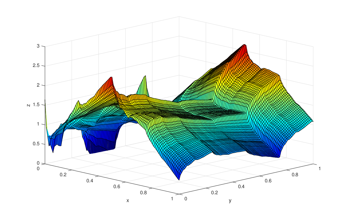
We simulate a random field on a planar graph G=(V,E)G=(V,E) which represents the administrative divisions in the Sydney bay area on the statistical area level 1. See the website of the Australian bureau of statistics (www.abs.gov.au) for further reference. It comprises 7,713 nodes and approximately 47k edges in total. Hence, GG is highly connected relative to the four-nearest neighbour structure. Figure 1(a) illustrates the graph.

We model a three-dimensional Markov random field Z=(Z1,Z2,Z3)Z=(Z_{1},Z_{2},Z_{3}). Every ZiZ_{i} has a specification as in (4.1) such that the marginals Zi​(s)Z_{i}(s) within each component are standard normally distributed. The parameter space of η\eta is derived from the adjacency matrix of the graph GG and contains the interval (−0.2221,0.1312)(-0.2221,0.1312). Note that the range for the lattice with a four-nearest-neighbourhood structure is (−0.25,0.25)\left(-0.25,0.25\right).

Then we adjust the marginal conditional variance τi2​(s)\tau^{2}_{i}(s) of the variable Zi​(s)Z_{i}(s) such that the entire random vector ZiZ_{i} has a covariance structure of the type Σi\Sigma_{i} as in (4.2).

Refer to caption
(a) The Sydney bay area (on statistical area level 1-scale)
Refer to caption
(b) Function plot of mm
Figure 1: Input graph and regression function for the bivariate regression problem
Refer to caption
(a) Estimate of m{m} with the D4 scaling function for j=2j=2
Refer to caption
(b) Estimate of m{m} with the Haar scaling function for j=3j=3
Figure 2: Estimated regression functions for a bivariate regression problem
Estimates on the graph Independent reference estimates
j D4 wavelet Haar wavelet D4 wavelet Haar wavelet
1 0.264 0.413 0.260 0.406
(0.006) (0.008) (0.006) (0.007)
2 0.122 0.258 0.119 0.254
(0.009) (0.008) (0.009) (0.007)
3 0.163 0.198 0.170 0.196
(0.036) (0.010) (0.044) (0.010)
4 0.422 0.259 0.435 0.257
(0.075) (0.012) (0.077) (0.012)
Table 1: L2L^{2}-error of the bivariate regression problem: the estimated mean and in parentheses the estimated standard deviation for a level j=1,…,4j=1,\ldots,4. The first two columns give the results for the random field, the last two columns those of the independent reference sample.

In order to obtain dependent components Z1Z_{1} and Z2Z_{2}, we draw the error terms from a two-dimensional Gaussian copula in each iteration. The exact simulation parameters are given by μZi=0\mu_{Z_{i}}=0, σi=1\sigma_{i}=1 for i=1,2,3i=1,2,3, η1=0.12\eta_{1}=0.12, η2=−0.18\eta_{2}=-0.18 and η3=0.12\eta_{3}=0.12. The covariance between the first two components is 0.7. The third component Z3Z_{3} is simulated as independent. The vectors τi2∈ℝ|V|\tau^{2}_{i}\in\mathbb{R}^{|V|} are computed with the formula τi2​(s)={diag∼⁡(inv​(I−ηi​H))}−1​(s)\tau_{i}^{2}(s)=\{\operatorname{diag}^{\sim}(\text{inv}(I-\eta_{i}H)\,)\}^{-1}(s) for i=1,2,3i=1,2,3. Here we denote the inverse of a matrix by inv\operatorname{inv}, the operator that maps the diagonal of a matrix to a vector by diag∼\operatorname{diag}^{\sim} and the elementwise inversion of a vector by {⋅}−1\{\cdot\}^{-1}. Afterwards, we transform the first two components Z1Z_{1} and Z2Z_{2} with the distribution function of a two-dimensional standard normal distribution onto the unit square and obtain the random field (X1,X2)(X_{1},X_{2}). We specify the mean function in this example as

m:ℝ2→ℝ,(x1,x2)↦(2−3​x22+4​x24)​exp⁡(−(2​x1−1)2).m\colon\mathbb{R}^{2}\rightarrow\mathbb{R},\,(x_{1},x_{2})\mapsto(2-3x_{2}^{2}+4x_{2}^{4})\,\exp\big(-(2x_{1}-1)^{2}\big).

Figure 1(b) shows the function plot of mm. We simulate Y⁡(s)=m⁡(X1​(s),X2​(s))+Z3​(s)Y(s)=m(X_{1}(s),X_{2}(s))+Z_{3}(s) and we use two different wavelet scaling functions for the estimation of mm: we perform the first regression with the Haar scaling function φ=1[0,1)\varphi=1_{[0,1)} and the second with Daubechies 4-scaling function D​4D4 (which is also known as d​b​2db2). Figure 2 displays the results: Figure 2(a) depicts the estimate with Daubechies 4-scaling function, Figure 2(b) the one with the Haar scaling function. Table 1 gives the L2L^{2}-error statistics. Note that the L2L^{2}-error minimizing jj for the Haar wavelet differs from the jj minimizing the error for Daubechies 4-scaling function. Moreover, the D​4D4 wavelet outperforms the Haar scaling function in this example. Table 1 also shows the L2L^{2}-error statistics for the same regression problem but with i.i.d. data of the same sample size. Note that the estimator obtained from i.i.d. data is slightly better than the estimate from the random field for both wavelet types.

Example 4.2 (Univariate non-parametric regression).

In this example we consider a one-dimensional spatial regression problem based on a graph which represents Australia divided into administrative divisions on the statistical area level 3. The graph consists of 330 nodes and 1600 edges, cf. Figure 3(a). This graph is highly connected in certain regions relative to the four-nearest neighbour structure on a lattice.

Refer to caption
(a) Administrative divisions of mainland Australia
Refer to caption
(b) A realization of XX and the mean function mm
Figure 3: Graph and true regression function.
Refer to caption
(a) Estimate of m{m} with the D4 scaling function for j=3,4,5j=3,4,5.
Refer to caption
(b) Estimate of m{m} with the Haar scaling function for j=3,4,5j=3,4,5.
Figure 4: The estimates for the univariate regression problem.

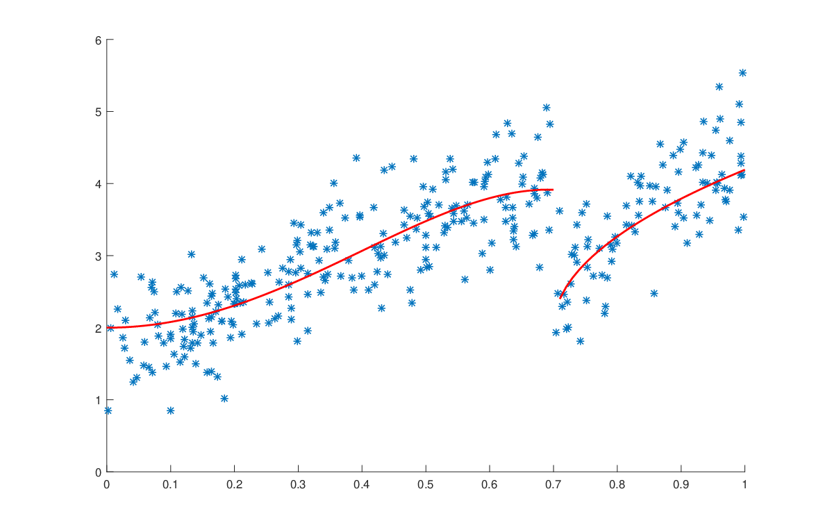
We simulate two Gaussian random fields Z1Z_{1} and Z2Z_{2} on GG with marginal means 0 and marginal variances 1 with the Markov chain method as in Example 4.1. The parameter space for η\eta contains the interval (−0.3060,0.1615)(-0.3060,0.1615). We choose η\eta for both components equal to 0.15 and run 15​k15k iterations of the MCMC-algorithm. Then we use the inverse of the standard normal distribution to retransform the component Z1Z_{1} onto the unit interval and obtain the random field XX with marginals uniformly distributed on [0,1][0,1]. The conditional mean function is defined as the discontinuous function

m:[0,1]→ℝ,x↦(2+8x2−(1.7x)4)1{x≤0.7}+2(4​(x−0.7)+1)1{0.7<x}.m\colon[0,1]\rightarrow\mathbb{R},\,x\mapsto\big(2+8x^{2}-(1.7x)^{4}\big)1_{\{x\leq 0.7\}}+2\big(\sqrt{4(x-0.7)}+1\big)1_{\{0.7<x\}}.

We define Y⁡(s)=m⁡(X⁡(s))+Z2​(s)/2Y(s)=m(X(s))+Z_{2}(s)/2. Figure 3(b) depicts the simulated random field. Figure 4(a) shows the estimation with the Daubechies 4-scaling function, while Figure 4(b) depicts the result for the Haar wavelet. We infer from Table 2 that the L2L^{2}-error is minimized for the level j=4j=4 in all cases. Note that in this example the Daubechies wavelet always outperforms the Haar wavelet when measured by the L2L^{2}-error. Again, the L2L^{2}-error of the independent reference estimate is slightly better in each case.

Estimates on the graph Independent reference estimates
j D4 wavelet Haar wavelet D4 wavelet Haar wavelet
2 0.326 0.405 0.321 0.401
(0.031) (0.059) (0.029) (0.061)
3 0.241 0.344 0.233 0.341
(0.033) (0.064) (0.035) (0.067)
4 0.224 0.284 0.213 0.280
(0.077) (0.073) (0.062) (0.078)
5 0.319 0.349 0.299 0.333
(0.172) (0.117) (0.134) (0.093)
6 0.772 0.753 0.712 0.727
(0.437) (0.213) (0.380) (0.212)
Table 2: L2L^{2}-error of the univariate regression problem: the estimated mean and in parentheses the estimated standard deviation for a level j=2,…,6j=2,\ldots,6. The first two columns give the results for the random field, the last two columns those of an independent reference sample of the same size.

5 Proofs of the Results in Section 2 and Section 3

The first lemma is a consequence of the coupling lemma of [3]. In the case of β\beta-mixing, we construct another sample (X∗,Y∗)(X^{*},Y^{*}) which has good properties.

Lemma 5.1.

Let (X,Y)(X,Y) be a random field on ℤN\mathbb{Z}^{N}. For each n∈ℕ+Nn\in\mathbb{N}_{+}^{N} and q∈ℕ+q\in\mathbb{N}_{+} such that 2q<min{ni:i=1,…,N}2q<\min\{n_{i}:i=1,\ldots,N\}, there is a partition of InI_{n} which is denoted by {I(l,u):l=1,…,2N,u=1,…,R}\{I(l,u):l=1,\ldots,2^{N},u=1,\ldots,R\} and collection of random variables Z∗(l,u)=((X∗(s),Y∗(s)):s∈I(l,u))∈ℝ(d+1)​qNZ^{*}(l,u)=((X^{*}(s),Y^{*}(s)):s\in I(l,u))\in\mathbb{R}^{(d+1)q^{N}} such that for each ll the collection Z∗​(l,1),…,Z∗​(l,R)Z^{*}(l,1),\ldots,Z^{*}(l,R) is independent and ℙ⁡(Z∗​(l,u)≠Z⁡(l,u))=β⁡(q)\mathbb{P}(Z^{*}(l,u)\neq Z(l,u))=\beta(q) where Z(l,u)=((X(s),Y(s)):s∈I(l,u))Z(l,u)=((X(s),Y(s)):s\in I(l,u)) and β\beta is the β\beta-mixing coefficient of (X,Y)(X,Y). Moreover, Z∗​(l,u)Z^{*}(l,u) is independent of Z⁡(l,1),…,Z⁡(l,u−1)Z(l,1),\ldots,Z(l,u-1) for each u=1,…,Ru=1,\ldots,R and for each l=1,…,2Nl=1,\ldots,2^{N}.

Proof.

The proof follows as in [8] where a similar coupling result is established under the α\alpha-mixing condition. We only sketch the main parts. Firstly, we give the construction of the partition. We choose R1,…,RNR_{1},\ldots,R_{N} such that

2​q​(Ri−1)<ni≤2​q​Ri=:ni∗​ for each ​k=1,…,N.2q(R_{i}-1)<n_{i}\leq 2qR_{i}=:n_{i}^{*}\text{ for each }k=1,\ldots,N.

For the kk-th coordinate direction, we partition the summation index set {1,…,ni∗}⊇{1,…,ni}\{1,\ldots,n_{i}^{*}\}\supseteq\{1,\ldots,n_{i}\} into RiR_{i} subsets each consisting of two disjoint intervals of length qq. So, we have a union of 2​Ri2R_{i} intervals of length qq.

Combining the partitions in all NN coordinate directions, we get a partition of the NN-dimensional rectangle In∗={s∈ℤN;eN≤s≤n∗}⊇InI_{n^{*}}=\{s\in\mathbb{Z}^{N};e_{N}\leq s\leq n^{*}\}\supseteq I_{n} into R=R1⋅…⋅RNR=R_{1}\cdot\ldots\cdot R_{N} blocks containing (2​q)N(2q)^{N} points of the NN-dimensional integer lattice each. Within each block, there are 2N2^{N} smaller subsets, which are NN-dimensional rectangles with all edges of length qq. Write I⁡(l,u)I(l,u) for the ll-th subset in the uu-th block, l=1,…,2Nl=1,\ldots,2^{N} and u=1,…,Ru=1,\ldots,R. Its cardinality is qNq^{N}. Moreover, using the requirement on nn, we have that Ri≥2R_{i}\geq 2 for each k=1,…,2Nk=1,\ldots,2^{N}. Thus, qN​R≤|In|q^{N}R\leq|I_{n}| and |In|/2N≤qN​R|I_{n}|/2^{N}\leq q^{N}R. The subcubes I⁡(l,u)I(l,u) have the property that for fixed ll the distance between I⁡(l,u)I(l,u) and I⁡(l,u′)I(l,u^{\prime}) is at least qq.

Secondly, we apply recursively (as in [8]) the lemma of [3] to the collection of random variables Z⁡(l,1),…,Z⁡(l,R)Z(l,1),\ldots,Z(l,R) for each ll. We obtain random variables Z∗​(l,1),…,Z∗​(l,R)∈ℝ(d+1)​qNZ^{*}(l,1),\ldots,Z^{*}(l,R)\in\mathbb{R}^{(d+1)q^{N}} with the desired properties. The claim follows now when defining the X∗​(s)X^{*}(s) and the Y∗​(s)Y^{*}(s) such that Z∗(l,u)=((X∗(s),Y∗(s)):s∈I(l,u))Z^{*}(l,u)=((X^{*}(s),Y^{*}(s)):s\in I(l,u)) a.s.a.s. for each u=1,…,Ru=1,\ldots,R and for each l=1,…,2Nl=1,\ldots,2^{N}. ∎

The next proposition is a well-known result of [22] which states sufficient conditions for a consistent estimator. It holds as well for dependent data because in the proof of the proposition those terms which are related to the dependence structure of the data converge to zero by assumption. So it is our task to verify these assumptions later. More precisely, it is assumed that the function classes can approximate the regression function mm arbitrarily exactly both in part (a) and in part (b) of this proposition. In our case this assumption does not depend on the data. However, the second requirement in both parts of the proposition is affected by the dependence structure of the data: here it is assumed that a certain empirical mean uniformly converges to the corresponding true mean for each possible function in the sieve. This requirement crucially depends on the data and we can verify this assumption later.

Proposition 5.2 (Modified version of [22] Theorem 10.2).

Let (Ω,𝒜,ℙ)(\Omega,\mathcal{A},\mathbb{P}) be a probability space endowed with the random field (X,Y)(X,Y) which satisfies the model (1.1) and Condition 2.1 such that each X⁡(s)X(s) is ℝd\mathbb{R}^{d}-valued and each Y⁡(s)Y(s) is ℝ\mathbb{R}-valued. Let ℱn⁡(k)⊆L2​(μX)\mathcal{F}_{n(k)}\subseteq L^{2}\left(\mu_{X}\right) be a class of functions f:ℝd→ℝf:\mathbb{R}^{d}\rightarrow\mathbb{R} for each k∈ℕ+k\in\mathbb{N}_{+}. Let (ρn⁡(k):k∈ℕ)⊆ℝ+(\rho_{n(k)}:k\in\mathbb{N})\subseteq\mathbb{R}_{+} be an sequence which increases to infinity. Denote the truncated least-squares estimate of mm from (2.7) by m^n\hat{m}_{n}. In addition, let the map from (2.6) be 𝒜\mathcal{A}-ℬ⁡(ℝ)\mathcal{B}(\mathbb{R})-measurable.

(a) If for all L>0L>0 both

limn→∞𝔼⁡[inff∈ℱn,‖f‖∞≤ρn‖f−m‖L2​(μX)]=0​ and\displaystyle\lim_{n\rightarrow\infty}\mathbb{E}\left[\,\inf_{f\in\mathcal{F}_{n},||f||_{\infty}\leq\rho_{n}}\left\lVert f-m\right\rVert_{L^{2}(\mu_{X})}\,\right]=0\text{ and }
limn→∞𝔼[supf∈Tρn​ℱn||In|−1∑s∈In(TLY(s)−f(X(s)))2\displaystyle\lim_{n\rightarrow\infty}\mathbb{E}\Biggl[\sup_{f\in T_{\rho_{n}}\mathcal{F}_{n}}\Bigg||I_{n}|^{-1}\sum_{s\in I_{n}}\Big(T_{L}Y(s)-f(X(s))\Big)^{2}
−𝔼[(TLY(eN)−f(X(eN))2]|]=0,\displaystyle\qquad\qquad\qquad\qquad\qquad\qquad-\mathbb{E}\left[\,\Big(T_{L}Y(e_{N})-f(X(e_{N})\Big)^{2}\,\right]\Bigg|\Biggl]=0,

then limn→∞𝔼⁡[∫ℝd(m^n−m)2​d​μX]=0\lim_{n\rightarrow\infty}\mathbb{E}\left[\,\int_{\mathbb{R}^{d}}\left(\hat{m}_{n}-m\right)^{2}\mathrm{d}\mu_{X}\,\right]=0.

(b) If limn→∞|In|−1​∑s∈In|Y⁡(s)−TL​Y​(s)|2=𝔼⁡[|Y⁡(eN)−TL​Y​(eN)|2]\lim_{n\rightarrow\infty}|I_{n}|^{-1}\sum_{s\in I_{n}}|Y(s)-T_{L}Y(s)|^{2}=\mathbb{E}\left[\,|Y(e_{N})-T_{L}Y(e_{N})|^{2}\,\right] a.s. and if

limn→∞inff∈ℱn,‖f‖∞≤ρn‖f−m‖L2​(μX)=0a.s. and\displaystyle\lim_{n\rightarrow\infty}\inf_{f\in\mathcal{F}_{n},||f||_{\infty}\leq\rho_{n}}\left\lVert f-m\right\rVert_{L^{2}(\mu_{X})}=0\quad a.s.\text{ and }
limn→∞supf∈Tρn​ℱn||In|−1∑n∈In(TLY(s)−f(X(s)))2\displaystyle\lim_{n\rightarrow\infty}\sup_{f\in T_{\rho_{n}}\mathcal{F}_{n}}\Bigg||I_{n}|^{-1}\sum_{n\in I_{n}}\Big(T_{L}Y(s)-f(X(s))\Big)^{2}
−𝔼[(TLY(eN)−f(X(eN)))2]|=0a.s.\displaystyle\qquad\qquad\qquad\qquad-\mathbb{E}\left[\,\Big(T_{L}Y(e_{N})-f(X(e_{N}))\Big)^{2}\,\right]\Bigg|=0\quad a.s.

for all L>0L>0, then limn→∞∫ℝd(m^n−m)2​d​μX=0\lim_{n\rightarrow\infty}\int_{\mathbb{R}^{d}}\left(\hat{m}_{n}-m\right)^{2}\mathrm{d}\mu_{X}=0 a.s.a.s.

We proceed with the proof of the first main theorem of Section 2.

Proof of Theorem 2.3.

We verify that in both dependence scenarios the sufficient criteria of Proposition 5.2 are satisfied for the given choices of the parameters. The structure of the proof is quite similar to the one of Theorem 10.3 in [22]. Therefore we sketch those parts which differ because of the dependence in the data and the assumed covering condition (Condition 2.2). The approximation property of the function classes is satisfied by assumption. Moreover, we can assume w.l.o.g. that L<ρnL<\rho_{n} in both cases because ρn\rho_{n} tends to infinity. We have to consider the function classes

ℋn\displaystyle\mathcal{H}_{n} ≔{h:ℝd×ℝ→ℝ,h(x,y)=|f(x)−TL(y)|2\displaystyle\coloneqq\big\{h:\mathbb{R}^{d}\times\mathbb{R}\rightarrow\mathbb{R},h(x,y)=|f(x)-T_{L}(y)|^{2}
 for all (x,y)∈ℝd×ℝ, for some f∈Tρnℱn}.\displaystyle\qquad\qquad\qquad\qquad\text{ for all }(x,y)\in\mathbb{R}^{d}\times\mathbb{R},\text{ for some }f\in T_{\rho_{n}}\mathcal{F}_{n}\big\}.

We begin with the case of α\alpha-mixing data. From Condition 2.2 we obtain a uniform bound on the ε\varepsilon-covering number 𝖭⁡(ε,ℋn,‖⋅‖L1​(ν))\mathsf{N}\big(\varepsilon,\mathcal{H}_{n},\left\lVert\,\cdot\,\right\rVert_{L^{1}(\nu)}\big) which we denote by Hℋn​(ε)H_{\mathcal{H}_{n}}(\varepsilon), here ν\nu is an arbitrary probability measure with equal mass concentrated at certain points z1,…,zu∈ℝz_{1},\ldots,z_{u}\in\mathbb{R}, u∈ℕ+u\in\mathbb{N}_{+}. Provided that L≤ρnL\leq\rho_{n}, we have for the covering number of this class ℋn\mathcal{H}_{n}

Hℋn​(ε32)≤HTρn​ℱn​(ε32​(4​ρn))=HTρn​ℱn​(ε128​ρn)=exp⁡κk​(ε/32,ρn).H_{\mathcal{H}_{n}}\left(\frac{\varepsilon}{32}\right)\leq H_{T_{\rho_{n}}\mathcal{F}_{n}}\left(\frac{\varepsilon}{32(4\rho_{n})}\right)=H_{T_{\rho_{n}}\mathcal{F}_{n}}\left(\frac{\varepsilon}{128\rho_{n}}\right)=\exp\kappa_{k}(\varepsilon/32,\rho_{n}).

For details on the first inequality, see the proof of Theorem 10.3 in [22]. Note that the functions in ℋn\mathcal{H}_{n} are bounded by 4​ρn24\rho_{n}^{2} if L≤ρnL\leq\rho_{n}. By assumption, ρn4​κn​(ε/32,ρn)​(log⁡|In|)2/|In|1/N→0​ as ​n→∞.\rho_{n}^{4}\kappa_{n}(\varepsilon/32,\rho_{n})\,\left(\log|I_{n}|\right)^{2}\,\big/\,|I_{n}|^{1/N}\rightarrow 0\text{ as }n\rightarrow\infty. We use Theorem A.4 to give an upper bound on the following probability (note that we only need to consider the exponential term in (A.2) which decays at a slower rate)

ℙ(supf∈Tρn​ℱn|1|In|∑s∈In|f(X(s))−TLY(s)|2−𝔼[|f(X(eN))−TLY(eN)|2]|>ε)\displaystyle\begin{split}&\mathbb{P}\Biggl(\sup_{f\in T_{\rho_{n}}\mathcal{F}_{n}}\Biggl|\frac{1}{|I_{n}|}\sum_{s\in I_{n}}\left|f(X(s))-T_{L}Y(s)\right|^{2}\\ &\qquad\qquad\qquad\qquad\qquad\qquad-\mathbb{E}\left[\,\left|f(X(e_{N}))-T_{L}Y(e_{N})\right|^{2}\,\right]\Biggl|>\varepsilon\Biggl)\end{split} (5.1)
≤A1​exp⁡{κn​(ε/32,ρn)}​exp​{−A2​|In|1/N​ε216​ρn4+4​ρn2​ε​(log⁡|In|)2}=A1exp{−ε2​|In|1/N16​ρn4+4​ρn2​ε​(log⁡|In|)2(A2−κn​(ε/32,ρn)​[16​ρn4+4​ρn2​ε​(log⁡|In|)2]ε2​|In|1/N)},\displaystyle\begin{split}&\leq A_{1}\,\exp\left\{\kappa_{n}(\varepsilon/32,\rho_{n})\right\}\,\exp\left\{-\frac{A_{2}\,|I_{n}|^{1/N}\,\varepsilon^{2}}{16\rho_{n}^{4}+4\rho_{n}^{2}\varepsilon\left(\log|I_{n}|\right)^{2}}\right\}\\ &=A_{1}\exp\Biggl\{-\frac{\varepsilon^{2}\,|I_{n}|^{1/N}}{16\rho_{n}^{4}+4\rho_{n}^{2}\varepsilon\left(\log|I_{n}|\right)^{2}}\\ &\qquad\qquad\qquad\qquad\left(A_{2}-\frac{\kappa_{n}(\varepsilon/32,\rho_{n})[16\rho_{n}^{4}+4\rho_{n}^{2}\varepsilon\left(\log|I_{n}|\right)^{2}]}{\varepsilon^{2}\,|I_{n}|^{1/N}}\right)\Biggl\},\end{split} (5.2)

for suitable constants A1A_{1} and A2A_{2}. The weak consistency follows from (5.2): let ε>0\varepsilon>0 be arbitrary but fixed, then

𝔼⁡[supf∈Tρn​ℱn|1|In|​∑s∈In|f⁡(X⁡(s))−TL​Y​(s)|2−𝔼⁡[|f⁡(X⁡(eN))−TL​Y​(eN)|2]|]\displaystyle\mathbb{E}\left[\,\sup_{f\in T_{\rho_{n}}\mathcal{F}_{n}}\left|\frac{1}{|I_{n}|}\sum_{s\in I_{n}}\left|f(X(s))-T_{L}Y(s)\right|^{2}-\mathbb{E}\left[\,\left|f(X(e_{N}))-T_{L}Y(e_{N})\right|^{2}\,\right]\right|\,\right]
≤ε+A1​exp⁡{κn​(ε,ρn)}​∫ε∞exp⁡{−A2​|In|1/N​t216​ρn4+4​ρn2​t​(log⁡|In|)2}​𝑑t→ε,\displaystyle\leq\varepsilon+A_{1}\exp\left\{\kappa_{n}(\varepsilon,\rho_{n})\right\}\,\int_{\varepsilon}^{\infty}\exp\left\{-\frac{A_{2}\,|I_{n}|^{1/N}\,t^{2}}{16\rho_{n}^{4}+4\rho_{n}^{2}t\left(\log|I_{n}|\right)^{2}}\right\}\mathrm{d}t\rightarrow\varepsilon,

as n→∞n\rightarrow\infty. Concerning the a.s.a.s. convergence of the estimate, we find that under the condition of α\alpha-mixing and stationarity the random variables {|Y⁡(s)−TL​Y​(s)|2:s∈ℤN}\{\left|Y(s)-T_{L}Y(s)\right|^{2}:s\in\mathbb{Z}^{N}\} are ergodic, see Theorem B.4 in [37]. This implies that

limn→∞|In|∑s∈In−1⁡|Y⁡(s)−TL​Y​(s)|2=𝔼⁡[|Y⁡(eN)−TL​Y​(eN)|2]a.s.\lim_{n\rightarrow\infty}|I_{n}|^{-1}\sum_{s\in I_{n}}|Y(s)-T_{L}Y(s)|^{2}=\mathbb{E}\left[\,|Y(e_{N})-T_{L}Y(e_{N})|^{2}\,\right]\quad a.s.

for all L>0L>0. Furthermore, if additionally

ρn4​(log⁡|In|)4/|In|1/N→0​ as ​n→∞,\rho_{n}^{4}\left(\log|I_{n}|\right)^{4}/|I_{n}|^{1/N}\rightarrow 0\text{ as }n\rightarrow\infty,

(5.2) remains summable for a sequence of index sets In⁡(k)I_{n(k)} which satisfies the condition in (2.1). Thus, an application of the Borel-Cantelli Lemma to the same equation yields that the estimator is strongly universally consistent. This finishes the case for α\alpha-mixing data.

Now consider the case of β\beta-mixing data. Again, we assume that ρn>L\rho_{n}>L. Therefore we use the partition of InI_{n} which is provided by Lemma 5.1 for the choice q=⌈2​log⁡|In|/c1⌉q=\lceil 2\log|I_{n}|/c_{1}\rceil. As in [49] we assume that Ri​q=niR_{i}q=n_{i} for each i=1,…,Ni=1,\ldots,N. We use the coupled random field (X∗,Y∗)(X^{*},Y^{*}) to obtain the estimator m^n∗\hat{m}^{*}_{n} of the regression function mm. We split the integrated error as follows

∫ℝd|m^n−m|2​d​μX≤2​∫ℝd|m^n∗−m|2​d​μX+2​∫ℝd|m^n∗−m^n|2​d​μX\displaystyle\int_{\mathbb{R}^{d}}|\hat{m}_{n}-m|^{2}\mathrm{d}\mu_{X}\leq 2\int_{\mathbb{R}^{d}}|\hat{m}^{*}_{n}-m|^{2}\mathrm{d}\mu_{X}+2\int_{\mathbb{R}^{d}}|\hat{m}^{*}_{n}-\hat{m}_{n}|^{2}\mathrm{d}\mu_{X} (5.3)

Exploiting the properties of (X∗,Y∗)(X^{*},Y^{*}), we find that the second term is at most

∫ℝd|m^n∗−m^n|2dμX≤4ρn2{(X∗(s),Y∗(s))≠(X(s),Y(s)) for one s∈In}.\int_{\mathbb{R}^{d}}|\hat{m}^{*}_{n}-\hat{m}_{n}|^{2}\mathrm{d}\mu_{X}\leq 4\rho_{n}^{2}\,\mathds{1}\!\left\{(X^{*}(s),Y^{*}(s))\neq(X(s),Y(s))\text{ for one }s\in I_{n}\right\}.

Using that β⁡(q)∈𝒪⁡(|In|−2)\beta(q)\in\mathcal{O}(|I_{n}|^{-2}), we have the following bound for the expectation

𝔼⁡[∫ℝd|m^n∗−m^n|2​d​μX]\displaystyle\mathbb{E}\left[\,\int_{\mathbb{R}^{d}}|\hat{m}^{*}_{n}-\hat{m}_{n}|^{2}\mathrm{d}\mu_{X}\,\right] ≤4​ρn2​β​(q)≤C​ρn2/|In|2→0,n→∞,\displaystyle\leq 4\rho_{n}^{2}\beta(q)\leq C\rho_{n}^{2}/|I_{n}|^{2}\rightarrow 0,\quad n\rightarrow\infty,

where we use that by assumption ρn4/|In|\rho_{n}^{4}/|I_{n}| vanishes. Moreover, we have

∑k=1∞ℙ⁡(∫ℝd|m^n⁡(k)∗−m^n⁡(k)|2​d​μX>ε)\displaystyle\sum_{k=1}^{\infty}\mathbb{P}\left(\int_{\mathbb{R}^{d}}|\hat{m}^{*}_{n(k)}-\hat{m}_{n(k)}|^{2}\mathrm{d}\mu_{X}>\varepsilon\right)
≤4​ε−1​∑k=1∞ρn⁡(k)2​β​(q⁡(n⁡(k)))≤C​∑k=1∞|In⁡(k)|−1.5<∞.\displaystyle\leq 4\varepsilon^{-1}\sum_{k=1}^{\infty}\rho_{n(k)}^{2}\beta(q(n(k)))\leq C\sum_{k=1}^{\infty}|I_{n(k)}|^{-1.5}<\infty.

Hence, ∫ℝd|m^n∗−m^n|2​d​μX\int_{\mathbb{R}^{d}}|\hat{m}^{*}_{n}-\hat{m}_{n}|^{2}\mathrm{d}\mu_{X} both vanishes in the mean and a.s.a.s. Consequently, the first integral in (5.3) remains and we need to study the probability in (5.1) in this scenario, it equals

ℙ(supf∈Tρn​ℱn|1|In|∑l=12N∑u=1R∑s∈I⁡(l,u)|f(X∗(s))−TLY∗(s)|2\displaystyle\mathbb{P}\Biggl(\sup_{f\in T_{\rho_{n}}\mathcal{F}_{n}}\Biggl|\frac{1}{|I_{n}|}\sum_{l=1}^{2^{N}}\sum_{u=1}^{R}\sum_{s\in I(l,u)}\left|f(X^{*}(s))-T_{L}Y^{*}(s)\right|^{2}
−𝔼[|f(X∗(eN))−TLY∗(eN)|2]|>ε)\displaystyle\qquad\qquad\qquad\qquad\qquad\qquad-\mathbb{E}\left[\,\left|f(X^{*}(e_{N}))-T_{L}Y^{*}(e_{N})\right|^{2}\,\right]\Biggl|>\varepsilon\Biggl)
≤∑l=12Nℙ(supf∈Tρn​ℱn|1R∑u=1R(∑s∈I⁡(l,u)|f(X∗(s))−TLY∗(s)|2−𝔼[|f(X∗(eN))−TLY∗(eN)|2])|>|In|​ε2N​R).\displaystyle\begin{split}&\leq\sum_{l=1}^{2^{N}}\mathbb{P}\Biggl(\sup_{f\in T_{\rho_{n}}\mathcal{F}_{n}}\Biggl|\frac{1}{R}\sum_{u=1}^{R}\Biggl(\sum_{s\in I(l,u)}\left|f(X^{*}(s))-T_{L}Y^{*}(s)\right|^{2}\\ &\qquad\qquad\qquad\qquad\qquad\qquad-\mathbb{E}\left[\,\left|f(X^{*}(e_{N}))-T_{L}Y^{*}(e_{N})\right|^{2}\,\right]\Biggl)\Biggl|>\frac{|I_{n}|\varepsilon}{2^{N}R}\Biggl).\end{split} (5.4)

Using the properties of the coupled process and the stationarity of (X,Y)(X,Y), we see that the summands over the index sets I⁡(l,1),…,I⁡(l,R)I(l,1),\ldots,I(l,R) are i.i.d. for each l=1,…,2Nl=1,\ldots,2^{N}. Consequently, we can apply Theorem 9.1 in [22]. Note that in the proof of this theorem it is only necessary that the data is independent but not that it is identically distributed. Hence, we obtain for (5.4) the bound

2N+3​Hℋn​(ε​qN2N+3)​exp⁡(−ε2​|In|22​N+13​qN​ρn4)\displaystyle 2^{N+3}H_{\mathcal{H}_{n}}\left(\frac{\varepsilon q^{N}}{2^{N+3}}\right)\exp\left(-\frac{\varepsilon^{2}|I_{n}|}{2^{2N+13}q^{N}\rho_{n}^{4}}\right)
≤2N+3​HTρn​ℱn​(ε​qN2N+3​(4​ρn2))​exp⁡(−ε2​|In|22​N+13​qN​ρn4)\displaystyle\leq 2^{N+3}H_{T_{\rho_{n}}\mathcal{F}_{n}}\left(\frac{\varepsilon q^{N}}{2^{N+3}(4\rho_{n}^{2})}\right)\exp\left(-\frac{\varepsilon^{2}|I_{n}|}{2^{2N+13}q^{N}\rho_{n}^{4}}\right)
=2N+3​exp⁡(κn​(ε​qN2N+3,ρn)−ε2​|In|24​N+13​(c1)−N​(log⁡|In|)N​ρn4)\displaystyle=2^{N+3}\exp\left(\kappa_{n}\left(\frac{\varepsilon q^{N}}{2^{N+3}},\rho_{n}\right)-\frac{\varepsilon^{2}|I_{n}|}{2^{4N+13}(c_{1})^{-N}(\log|I_{n}|)^{N}\rho_{n}^{4}}\right)

using the definition of κn\kappa_{n} and of the block size qq. Note that the factor qNq^{N} inside κn\kappa_{n} can be neglected as it only decreases κn\kappa_{n} marginally if ε>0\varepsilon>0 is fixed. Now, the same computations as in the case of α\alpha-mixing data yield the result. We do not go into the details. ∎

The proof of Corollary 2.4 requires the concept of the Vapnik-Chervonenkis-dimension (VC-dimension). The definition of the VC-dimension is rather technical and can be found in the book of [22], Definition 9.6.

Proof of Corollary 2.4.

It remains to consider some technical issues. Clearly, the map

ℝKn×Ω∋(a,ω)↦∑i=1Knai​fi​(X⁡(s,ω))​ is ℬ⁡(ℝKn)⊗𝒜-measurable.\mathbb{R}^{K_{n}}\times\Omega\ni(a,\omega)\mapsto\sum_{i=1}^{K_{n}}a_{i}f_{i}(X(s,\omega))\text{ is $\mathcal{B}(\mathbb{R}^{K_{n}})\otimes\mathcal{A}$-measurable}.

The desired measurability of the map in (2.6) follows from the fact that for any measurable function gg on a product space (S×T,𝒮⊗𝒯)(S\times T,\mathcal{S}\otimes\mathcal{T}) the set

{t∈T:sups∈Sg⁡(s,t)>c}\displaystyle\left\{t\in T:\sup_{s\in S}g(s,t)>c\right\} ={t∈T|∃s∈S:g(s,t)>c}\displaystyle=\left\{t\in T\,\big|\,\exists s\in S:g(s,t)>c\right\}
=πTS×T​{(s,t)∈S×T:g⁡(s,t)>c}∈𝒯,\displaystyle=\pi^{S\times T}_{T}\{(s,t)\in S\times T:g(s,t)>c\}\in\mathcal{T},

where πTS×T\pi^{S\times T}_{T} is the projection from S×TS\times T onto TT.

Furthermore, the Vapnik-Chervonenkis-dimension is at least 2 if Kn≥2K_{n}\geq 2. Indeed, choose functions f1f_{1} and f2f_{2}. Without loss of generality, there is an x¯\bar{x} in ℝd\mathbb{R}^{d} and an aa in ℝ\mathbb{R} such that a​f1​(x¯)=f2​(x¯)>0af_{1}(\bar{x})=f_{2}(\bar{x})>0. Since f1f_{1} and f2f_{2} are linearly independent, exactly one of the following three cases occurs: (1) either there are x1x_{1} and x2x_{2} in a neighbourhood of x¯\bar{x} such that a​f1​(x1)>f2​(x1)af_{1}(x_{1})>f_{2}(x_{1}) and f2​(x2)>a​f1​(x2)f_{2}(x_{2})>af_{1}(x_{2}), (2) or a​f1=f2af_{1}=f_{2} on UU and a​f1>f2af_{1}>f_{2} on ℝd∖U\mathbb{R}^{d}\setminus U, where U⊂ℝdU\subset\mathbb{R}^{d} contains x¯\bar{x}, (3) or f2=a​f1f_{2}=af_{1} on UU and f2>a​f1f_{2}>af_{1} on ℝd∖U\mathbb{R}^{d}\setminus U. In the last two cases we can modify aa such that we achieve the first case, by linear independence. Thus, the two points pi≔(xi,ti)p_{i}\coloneqq(x_{i},t_{i}) (for i=1,2i=1,2) with the property that a​f1​(x1)>t1>f2​(x1)af_{1}(x_{1})>t_{1}>f_{2}(x_{1}) and f2​(x2)>t2>a​f1​(x2)f_{2}(x_{2})>t_{2}>af_{1}(x_{2}) are shattered by the set of all subgraphs of the linear space ⟨f1,f2⟩\langle f_{1},f_{2}\rangle, hence, 𝒱⟨f1,…,fn⟩+≥𝒱⟨f1,f2⟩+≥2\mathcal{V}_{\langle f_{1},\ldots,f_{n}\rangle^{+}}\geq\mathcal{V}_{\langle f_{1},f_{2}\rangle^{+}}\geq 2. Consequently, the conditions of Theorem A.1 are satisfied. We have

κn​(ε,ρn)=log⁡HTρn​ℱn​(ε4​ρn)\displaystyle\kappa_{n}(\varepsilon,\rho_{n})=\log H_{T_{\rho_{n}}\mathcal{F}_{n}}\left(\frac{\varepsilon}{4\rho_{n}}\right) ≤log⁡(3​(16​e​ρn2ε​log⁡24​e​ρn2ε)𝒱(Tρn​ℱn)+)\displaystyle\leq\log\left(3\left(\frac{16e\rho_{n}^{2}}{\varepsilon}\,\log\frac{24e\rho_{n}^{2}}{\varepsilon}\right)^{\mathcal{V}_{\left(T_{\rho_{n}}\mathcal{F}_{n}\right)^{+}}}\right)
≤log⁡3+(Kn+1)​log⁡((24)2​(eε)2​ρn4)\displaystyle\leq\log 3+(K_{n}+1)\log\left((24)^{2}\left(\frac{e}{\varepsilon}\right)^{2}\rho_{n}^{4}\right)
=𝒪⁡(Kn​log⁡ρn).\displaystyle=\mathcal{O}(K_{n}\log\rho_{n}).

The statement follows now from Theorem 2.3. ∎

We need another proposition and a piece of notation to prove the rate of convergence of the regression estimator.

Notation 5.3.

Let ff be a real-valued function on ℝd\mathbb{R}^{d} and let the distribution of the X⁡(s)X(s) be given by μX\mu_{X}. Let X′={X′​(s):s∈ℤN}X^{\prime}=\{X^{\prime}(s):s\in\mathbb{Z}^{N}\} be an i.i.d. ghost sample with the same marginals as XX. Moreover, X∗X^{*} is constructed for each n∈ℕ+Nn\in\mathbb{N}_{+}^{N} as in Lemma 5.1 and the random field X†X^{\dagger} is an independent copy of X∗X^{*}. Define the following empirical L2L^{2}-norms

‖f‖|In|≔(|In|−1∑s∈Inf(X(s))2)1/2,‖f‖|In|′≔(|In|−1∑s∈Inf(X′(s))2)1/2\displaystyle\left\lVert f\right\rVert_{|I_{n}|}\coloneqq\left(|I_{n}|^{-1}\sum_{s\in I_{n}}f(X(s))^{2}\right)^{1/2},\quad\left\lVert f\right\rVert^{{}^{\prime}}_{|I_{n}|}\coloneqq\left(|I_{n}|^{-1}\sum_{s\in I_{n}}f(X^{{}^{\prime}}(s))^{2}\right)^{1/2}
and ‖f‖|In|∼≔((2|In|)−1∑s∈Inf(X(s))2+f(X′(s))2)1/2\displaystyle\text{ and }\left\lVert f\right\rVert^{\sim}_{|I_{n}|}\coloneqq\left((2|I_{n}|)^{-1}\sum_{s\in I_{n}}f(X(s))^{2}+f(X^{{}^{\prime}}(s))^{2}\right)^{1/2}
as well as ​‖f‖|In|∗≔(|In|−1​∑s∈Inf​(X∗​(s))2)1/2\displaystyle\text{ as well as }\left\lVert f\right\rVert^{*}_{|I_{n}|}\coloneqq\left(|I_{n}|^{-1}\sum_{s\in I_{n}}f(X^{*}(s))^{2}\right)^{1/2}
and ​‖f‖|In|†≔(|In|−1​∑s∈Inf​(X†​(s))2)1/2.\displaystyle\text{ and }\left\lVert f\right\rVert^{\dagger}_{|I_{n}|}\coloneqq\left(|I_{n}|^{-1}\sum_{s\in I_{n}}f(X^{\dagger}(s))^{2}\right)^{1/2}.

Consider the random point measure ν\nu with equal masses which is induced by the sample of the random field and of the ghost sample (X⁡(In),X′​(In)CLOSE(X(I_{n}),X^{\prime}(I_{n}), i.e., ν=(2​|In|)−1​∑s∈In(δX⁡(s)+δX′​(s))\nu=(2|I_{n}|)^{-1}\sum_{s\in I_{n}}\big(\delta_{X(s)}+\delta_{X^{\prime}(s)}\big). We abbreviate the ε\varepsilon-covering number of a function class 𝒢\mathcal{G} w.r.t. 2-norm of ν\nu by

𝖭2(ε,𝒢,(X(In),X′(In)))≔𝖭(ε,𝒢,‖⋅‖L2​(ν)).\mathsf{N}_{2}\left(\varepsilon,\mathcal{G},(X(I_{n}),X^{{}^{\prime}}(I_{n}))\right)\coloneqq\mathsf{N}\left(\varepsilon,\mathcal{G},\left\lVert\,\cdot\,\right\rVert_{L^{2}(\nu)}\right).

The next two statements prepare the second main theorem of Section 2 which is Theorem 2.5. The first is intended for α\alpha-mixing data, the second for β\beta-mixing data.

Proposition 5.4.

Assume that the random field XX satisfies Condition 2.1 ( α ). Let 𝒢\mathcal{G} be a class of ℝ\mathbb{R}-valued functions on ℝd\mathbb{R}^{d} which are all bounded by a universal constant BB. Then for all ε>0\varepsilon>0

ℙ⁡(supf∈𝒢‖f‖−2​‖f‖In>ε)≤A1‖𝖭2(2​ε32,𝒢,(X(In),X′(In)))‖ℙ,∞⋅(exp⁡(−A2​ε4​|In|1/NB4+B2​ε2​(log⁡|In|)2)+exp⁡(−A3​ε2​|In|B2))\displaystyle\begin{split}&\mathbb{P}\left(\sup_{f\in\mathcal{G}}\;\left\lVert f\right\rVert-2\left\lVert f\right\rVert_{I_{n}}>\varepsilon\right)\\ &\leq A_{1}\left\lVert\mathsf{N}_{2}\left(\frac{\sqrt{2}\varepsilon}{32},\mathcal{G},(X(I_{n}),X^{{}^{\prime}}(I_{n}))\right)\right\rVert_{\mathbb{P},\infty}\\ &\quad\cdot\left(\exp\left(-\frac{A_{2}\varepsilon^{4}|I_{n}|^{1/N}}{B^{4}+B^{2}\,\varepsilon^{2}\left(\log|I_{n}|\right)^{2}}\right)+\exp\left(-\frac{A_{3}\varepsilon^{2}|I_{n}|}{B^{2}}\right)\right)\end{split} (5.5)

for constants 0<A1,A2,A3<∞0<A_{1},A_{2},A_{3}<\infty which neither depend on the bound BB, nor on ε\varepsilon, nor on the index set InI_{n}.

Provided that the Vapnik-Chervonenkis dimension 𝒱𝒢+\mathcal{V}_{\mathcal{G}^{+}} is at least 2 and that ε\varepsilon is sufficiently small, the bound from Proposition 5.4 is non-trivial: we have with Proposition A.1

log‖𝖭2(ε16​2,𝒢,(X(In),X′(In)))‖ℙ,∞\displaystyle\log\left\lVert\mathsf{N}_{2}\left(\frac{\varepsilon}{16\sqrt{2}},\mathcal{G},(X(I_{n}),X^{{}^{\prime}}(I_{n}))\right)\right\rVert_{\mathbb{P},\infty}
≤log⁡3+𝒱𝒢+​log⁡(163​e​B2ε2⋅log⁡24⋅162​e​B2ε2).\displaystyle\leq\log 3+\mathcal{V}_{\mathcal{G}^{+}}\log\left(\frac{16^{3}eB^{2}}{\varepsilon^{2}}\cdot\log\frac{24\cdot 16^{2}eB^{2}}{\varepsilon^{2}}\right).
Proof of Proposition 5.4.

Let {X⁡(s):s∈In}\{X(s):s\in I_{n}\} be a subset of the strongly mixing and stationary random field XX and let {X′(s):s∈In}\{X^{{}^{\prime}}(s):s\in I_{n}\} be the corresponding ghost sample. We use the relation

ℙ⁡(supf∈𝒢‖f‖−2​‖f‖In>ε)\displaystyle\mathbb{P}\left(\sup_{f\in\mathcal{G}}\;\left\lVert f\right\rVert-2\left\lVert f\right\rVert_{I_{n}}>\varepsilon\right)
≤ℙ⁡(supf∈𝒢‖f‖−2​‖f‖In′>ε2)+ℙ⁡(supf∈𝒢‖f‖In′−‖f‖In>ε4).\displaystyle\leq\mathbb{P}\left(\sup_{f\in\mathcal{G}}\;\left\lVert f\right\rVert-2\left\lVert f\right\rVert^{\prime}_{I_{n}}>\frac{\varepsilon}{2}\right)+\mathbb{P}\left(\sup_{f\in\mathcal{G}}\;\left\lVert f\right\rVert^{\prime}_{I_{n}}-\left\lVert f\right\rVert_{I_{n}}>\frac{\varepsilon}{4}\right).

We only consider the second probability on the right-hand-side of the last inequality, bounds on the first probability are given by the second term in the second line of (5.5) and are derived in Theorem 11.2 of [22]. Let U1,…,UH∗U_{1},\ldots,U_{H^{*}} be an ε/(16​2)\varepsilon/(16\sqrt{2})-covering of 𝒢\mathcal{G} with respect to the empirical L2L^{2}-norm of the sample (X(In),X′(In))\big(X(I_{n}),X^{{}^{\prime}}(I_{n})\big) with the definition H∗≔𝖭2(ε/(162),𝒢,(X(In),X′(In)))H^{*}\coloneqq\mathsf{N}_{2}\big(\varepsilon/(16\sqrt{2}),\mathcal{G},\big(X(I_{n}),X^{{}^{\prime}}(I_{n})\big)\big) and Uk≔{f∈𝒢:‖f−gk‖In∼<ε/(16​2)}U_{k}\coloneqq\{f\in\mathcal{G}:\left\lVert f-g_{k}\right\rVert^{\sim}_{I_{n}}<\varepsilon/(16\sqrt{2})\}, where the covering functions are g1,…​gH∗g_{1},\ldots g_{H^{*}}. Note that H∗H^{*} and the UkU_{k} are random and that both ‖⋅‖In\left\lVert\,\cdot\,\right\rVert_{I_{n}} and ‖⋅‖In′\left\lVert\,\cdot\,\right\rVert^{\prime}_{I_{n}} are bounded by 2​‖⋅‖In∼\sqrt{2}\left\lVert\,\cdot\,\right\rVert^{\sim}_{I_{n}}. Then,

ℙ(∃f∈𝒢:‖f‖In′−‖f‖In>ε4)\displaystyle\mathbb{P}\left(\exists f\in\mathcal{G}:\left\lVert f\right\rVert_{I_{n}}^{{}^{\prime}}-\left\lVert f\right\rVert_{I_{n}}>\frac{\varepsilon}{4}\right) ≤∑k=1‖H∗‖ℙ,∞ℙ(∃f∈Uk:‖f‖In′−‖f‖In>ε4).\displaystyle\leq\sum_{k=1}^{||H^{*}||_{\mathbb{P},\infty}}\mathbb{P}\left(\exists f\in U_{k}:\left\lVert f\right\rVert_{I_{n}}^{{}^{\prime}}-\left\lVert f\right\rVert_{I_{n}}>\frac{\varepsilon}{4}\right). (5.6)

Now, we use that ‖f‖In≤2​‖f‖In∼\left\lVert f\right\rVert_{I_{n}}\leq\sqrt{2}\left\lVert f\right\rVert_{I_{n}}^{\sim} to obtain for f∈Ukf\in U_{k} the inequality

‖f‖In′−‖f‖In\displaystyle\left\lVert f\right\rVert_{I_{n}}^{{}^{\prime}}-\left\lVert f\right\rVert_{I_{n}} =‖f‖In′−‖gk‖In′+‖gk‖In′−‖gk‖In+‖gk‖In−‖f‖In\displaystyle=\left\lVert f\right\rVert_{I_{n}}^{{}^{\prime}}-\left\lVert g_{k}\right\rVert_{I_{n}}^{{}^{\prime}}+\left\lVert g_{k}\right\rVert_{I_{n}}^{{}^{\prime}}-\left\lVert g_{k}\right\rVert_{I_{n}}+\left\lVert g_{k}\right\rVert_{I_{n}}-\left\lVert f\right\rVert_{I_{n}}
≤‖f−gk‖In′+(‖gk‖In′−‖gk‖In)+‖f−gk‖In\displaystyle\leq\left\lVert f-g_{k}\right\rVert_{I_{n}}^{{}^{\prime}}+\left(\left\lVert g_{k}\right\rVert_{I_{n}}^{{}^{\prime}}-\left\lVert g_{k}\right\rVert_{I_{n}}\right)+\left\lVert f-g_{k}\right\rVert_{I_{n}}
≤22ε16​2+(‖gk‖In′−‖gk‖In).\displaystyle\leq 2\sqrt{2}\,\frac{\varepsilon}{16\sqrt{2}}+\left(\left\lVert g_{k}\right\rVert_{I_{n}}^{{}^{\prime}}-\left\lVert g_{k}\right\rVert_{I_{n}}\right).

Hence, {∃f∈Uk:‖f‖In′−‖f‖In>ε4}\big\{\exists f\in U_{k}:\left\lVert f\right\rVert_{I_{n}}^{{}^{\prime}}-\left\lVert f\right\rVert_{I_{n}}>\frac{\varepsilon}{4}\big\} is a subset of {‖gk‖In′−‖g‖In>ε8}\big\{\left\lVert g_{k}\right\rVert_{I_{n}}^{{}^{\prime}}-\left\lVert g\right\rVert_{I_{n}}>\frac{\varepsilon}{8}\big\}. Since the inequality a−b>ca-b>c implies a2−b2>c2a^{2}-b^{2}>c^{2} for a,b,c≥0a,b,c\geq 0, we get for the probabilities on the right-hand-side of (5.6) the following bounds

ℙ(‖gk‖In′−‖gk‖In>ε8)≤ℙ((‖gk‖In′)2−(‖gk‖In)2>ε264)\displaystyle\mathbb{P}\left(\left\lVert g_{k}\right\rVert_{I_{n}}^{{}^{\prime}}-\left\lVert g_{k}\right\rVert_{I_{n}}>\frac{\varepsilon}{8}\right)\leq\mathbb{P}\left(\left(\left\lVert g_{k}\right\rVert_{I_{n}}^{{}^{\prime}}\right)^{2}-\left(\left\lVert g_{k}\right\rVert_{I_{n}}\right)^{2}>\frac{\varepsilon^{2}}{64}\right)
≤ℙ(1|In|∑s∈In{gk(X′(s))2−𝔼[gk(X′(eN))2]}\displaystyle\leq\mathbb{P}\Biggl(\frac{1}{|I_{n}|}\sum_{s\in I_{n}}\left\{g_{k}(X^{{}^{\prime}}(s))^{2}-\mathbb{E}\left[\,g_{k}(X^{{}^{\prime}}(e_{N}))^{2}\,\right]\right\}
−1|In|∑s∈In{gk(X(s))2−𝔼[gk(X(eN))2]}>ε264)\displaystyle\quad-\frac{1}{|I_{n}|}\sum_{s\in I_{n}}\left\{g_{k}(X(s))^{2}-\mathbb{E}\left[\,g_{k}(X(e_{N}))^{2}\,\right]\right\}>\frac{\varepsilon^{2}}{64}\Biggl)
≤ℙ(|1|In|∑s∈Ingk(X′(s))2−𝔼[gk(X′(eN))2]|>ε2128)+ℙ⁡(|1|In|​∑s∈Ingk​(X⁡(s))2−𝔼⁡[gk​(X⁡(eN))2]|>ε2128).\displaystyle\begin{split}&\leq\mathbb{P}\left(\left|\frac{1}{|I_{n}|}\sum_{s\in I_{n}}g_{k}(X^{{}^{\prime}}(s))^{2}-\mathbb{E}\left[\,g_{k}(X^{{}^{\prime}}(e_{N}))^{2}\,\right]\right|>\frac{\varepsilon^{2}}{128}\right)\\ &\quad+\mathbb{P}\left(\left|\frac{1}{|I_{n}|}\sum_{s\in I_{n}}g_{k}(X(s))^{2}-\mathbb{E}\left[\,g_{k}(X(e_{N}))^{2}\,\right]\right|>\frac{\varepsilon^{2}}{128}\right).\end{split} (5.7)

The first term from (5.7) can be bounded by Hoeffding’s inequality, we have

ℙ(|1|In|∑s∈Ingk(X′(s))2−𝔼[gk(X′(eN))2]|>ε2128)≤2exp(−Cε4|In|B4).\displaystyle\mathbb{P}\left(\left|\frac{1}{|I_{n}|}\sum_{s\in I_{n}}g_{k}(X^{{}^{\prime}}(s))^{2}-\mathbb{E}\left[\,g_{k}(X^{{}^{\prime}}(e_{N}))^{2}\,\right]\right|>\frac{\varepsilon^{2}}{128}\right)\leq 2\exp\left(-C\varepsilon^{4}\frac{|I_{n}|}{B^{4}}\right). (5.8)

We apply Proposition A.3 to the second term and obtain that

ℙ⁡(|1|In|​∑s∈Ingk​(X⁡(s))2−𝔼⁡[gk​(X⁡(s))2]|>ε2128)\displaystyle\mathbb{P}\left(\left|\frac{1}{|I_{n}|}\sum_{s\in I_{n}}g_{k}(X(s))^{2}-\mathbb{E}\left[\,g_{k}(X(s))^{2}\,\right]\right|>\frac{\varepsilon^{2}}{128}\right)
≤exp⁡(−C​ε4​|In|1/NB4+B2​ε2​(log⁡|In|)2).\displaystyle\leq\exp\left(-\frac{C\varepsilon^{4}|I_{n}|^{1/N}}{B^{4}+B^{2}\,\varepsilon^{2}\left(\log|I_{n}|\right)^{2}}\right). (5.9)

Obviously, the bound in (5.9) dominates the bound in (5.8). This finishes the proof. ∎

The next proposition is a generalization of Theorem 11.2 of [22] for β\beta-mixing data.

Proposition 5.5.

Assume that the random field XX satisfies Condition 2.1 ( β ). Let 𝒢\mathcal{G} be a class of ℝ\mathbb{R}-valued functions on ℝd\mathbb{R}^{d} which are all bounded by B∈ℝ+B\in\mathbb{R}_{+}. Let nn be sufficiently large such that both 8/c1log|In|<min{ni:i=1,…,N}8/c_{1}\log|I_{n}|<\min\{n_{i}:i=1,\ldots,N\} and C∗≤23​N−1​(c1)−N​(log⁡|In|)NC^{*}\leq 2^{3N-1}(c_{1})^{-N}(\log|I_{n}|)^{N} where the constant C∗C^{*} is defined in (5.12). Then for all ε>0\varepsilon>0

ℙ⁡(supf∈𝒢‖f‖−2​‖f‖In∗≥ε)≤3⋅2N‖𝖭2(2​ε32,𝒢,(X(In),X′(In)))‖ℙ,∞⋅exp⁡(−ε2​|In|25​N+5​B2​c1−N​(log⁡|In|)N)\displaystyle\begin{split}\mathbb{P}\left(\sup_{f\in\mathcal{G}}\;\left\lVert f\right\rVert-2\left\lVert f\right\rVert^{*}_{I_{n}}\geq\varepsilon\right)&\leq 3\cdot 2^{N}\left\lVert\mathsf{N}_{2}\left(\frac{\sqrt{2}\varepsilon}{32},\mathcal{G},(X(I_{n}),X^{{}^{\prime}}(I_{n}))\right)\right\rVert_{\mathbb{P},\infty}\\ &\quad\cdot\exp\left(-\frac{\varepsilon^{2}|I_{n}|}{2^{5N+5}B^{2}c_{1}^{-N}(\log|I_{n}|)^{N}}\right)\end{split} (5.10)
Proof of Proposition 5.5.

Set q=⌈2/c1​log⁡|In|⌉q=\lceil 2/c_{1}\log|I_{n}|\rceil and apply Lemma 5.1. We obtain a partition of InI_{n} given by {I(l,u):l=1,…,2N,u=1,…,R}\{I(l,u):l=1,\ldots,2^{N},u=1,\ldots,R\} such that we can write

|In|−1​∑s∈Inf​(X∗​(s))2=R−1​∑l=12N∑u=1RZ∗​(l,u)2\displaystyle|I_{n}|^{-1}\sum_{s\in I_{n}}f(X^{*}(s))^{2}=R^{-1}\sum_{l=1}^{2^{N}}\sum_{u=1}^{R}Z^{*}(l,u)^{2}\quad
and |In|−1​∑s∈Inf​(X†​(s))2=R−1​∑l=12N∑u=1RZ†​(l,u)2,\displaystyle\text{ and }\quad|I_{n}|^{-1}\sum_{s\in I_{n}}f(X^{\dagger}(s))^{2}=R^{-1}\sum_{l=1}^{2^{N}}\sum_{u=1}^{R}Z^{\dagger}(l,u)^{2},

where

Z∗​(l,u)=(R​|In|−1​∑s∈I⁡(l,u)f​(X∗​(s))2)1/2\displaystyle Z^{*}(l,u)=\left(R|I_{n}|^{-1}\sum_{s\in I(l,u)}f(X^{*}(s))^{2}\right)^{1/2}
and ​Z†​(l,u)=(R​|In|−1​∑s∈I⁡(l,u)f​(X†​(s))2)1/2.\displaystyle\text{ and }Z^{\dagger}(l,u)=\left(R|I_{n}|^{-1}\sum_{s\in I(l,u)}f(X^{\dagger}(s))^{2}\right)^{1/2}.

Note that 0≤Z∗​(l,u),Z†​(l,u)≤B0\leq Z^{*}(l,u),Z^{\dagger}(l,u)\leq B.

In the following, let f~\tilde{f} be a function in 𝒢\mathcal{G} such that ‖f~‖−2​‖f~‖In≥ε\left\lVert\tilde{f}\right\rVert-2\left\lVert\tilde{f}\right\rVert_{I_{n}}\geq\varepsilon if there is such a function. Otherwise, f~\tilde{f} is any other function. We write ℙ∗\mathbb{P}^{*} for the conditional probability measure and 𝔼∗\mathbb{E}^{*} for the conditional expectation given the data X∗​(In)X^{*}(I_{n}).

The remaining proof is a modification of Theorem 11.2 in [22] and is split in three steps. In the first step, we show that

ℙ⁡(supf∈𝒢‖f‖−2​‖f‖In∗≥ε)≤32​ℙ​(supf∈𝒢‖f‖In†−‖f‖In∗≥ε4),\displaystyle\mathbb{P}\left(\sup_{f\in\mathcal{G}}\;\left\lVert f\right\rVert-2\left\lVert f\right\rVert^{*}_{I_{n}}\geq\varepsilon\right)\leq\frac{3}{2}\mathbb{P}\left(\sup_{f\in\mathcal{G}}\;\left\lVert f\right\rVert^{\dagger}_{I_{n}}-\left\lVert f\right\rVert^{*}_{I_{n}}\geq\frac{\varepsilon}{4}\right), (5.11)

if B2/ε2≤|In|/(22​N+6​C∗)B^{2}/\varepsilon^{2}\leq|I_{n}|/(2^{2N+6}C^{*}) where

C∗≔2​1+Cℙ​(1+CN​β¯∞).\displaystyle C^{*}\coloneqq\sqrt{2}\sqrt{1+C_{\mathbb{P}}}(1+C_{N}\bar{\beta}_{\infty}). (5.12)

Here CℙC_{\mathbb{P}} is a uniform bound of the essential suprema of the Radon-Nikodým derivatives in (2.2) and the factor β¯∞\bar{\beta}_{\infty} equals ∑k=0∞kN−1​β⁡(k)<∞\sum_{k=0}^{\infty}k^{N-1}\sqrt{\beta(k)}<\infty; additionally, the constant CNC_{N} depends on the lattice dimension NN and is given below.

For this result, we need that

ℙ∗​(2​‖f~‖In†+ε2≥‖f~‖)≥1−ℙ∗​(3​‖f~‖2+ε24≤4​(‖f~‖2−(‖f~‖In†)2))\displaystyle\mathbb{P}^{*}\left(2\left\lVert\tilde{f}\right\rVert^{\dagger}_{I_{n}}+\frac{\varepsilon}{2}\geq\left\lVert\tilde{f}\right\rVert\right)\geq 1-\mathbb{P}^{*}\left(3\left\lVert\tilde{f}\right\rVert^{2}+\frac{\varepsilon^{2}}{4}\leq 4\left(\left\lVert\tilde{f}\right\rVert^{2}-\left(\left\lVert\tilde{f}\right\rVert^{\dagger}_{I_{n}}\right)^{2}\right)\right) (5.13)

Indeed, this follows with some calculations (see the proof of Theorem 11.2 [22]). Furthermore, we need a result, which follows using the β\beta-mixing property and a lemma in [38],

∑s,t∈I⁡(l,u)𝔼∗​[f~​(X†​(s))2​f~​(X†​(t))2]\displaystyle\sum_{s,t\in I(l,u)}\mathbb{E}^{*}\left[\,\tilde{f}(X^{\dagger}(s))^{2}\tilde{f}(X^{\dagger}(t))^{2}\,\right]
≤2​1+Cℙ​𝔼∗​[f~​(X†​(eN))4]​∑s,t∈I⁡(l,u)β​(‖s−t‖∞)1/2\displaystyle\leq\sqrt{2}\sqrt{1+C_{\mathbb{P}}}\mathbb{E}^{*}\left[\,\tilde{f}(X^{\dagger}(e_{N}))^{4}\,\right]\sum_{s,t\in I(l,u)}\beta(\left\lVert s-t\right\rVert_{\infty})^{1/2}
≤2​1+Cℙ​(1+CN​β¯∞)​B2​‖f~‖2​qN,\displaystyle\leq\sqrt{2}\sqrt{1+C_{\mathbb{P}}}(1+C_{N}\bar{\beta}_{\infty})B^{2}\left\lVert\tilde{f}\right\rVert^{2}q^{N},

for a certain constant CNC_{N} which depends on the lattice dimension NN.

Moreover, using that for a fixed ll the blocked random variables {X†(I(l,u)):u=1,…,R}\{X^{\dagger}(I(l,u)):u=1,\ldots,R\} are independent, the probability on the right-hand-side of (5.13) is at most

16|In|2​Var∗⁡(∑l,u∑s∈I⁡(l,u)f~​(X†​(s))2)(3​‖f~‖2+ε24)2\displaystyle\frac{16}{|I_{n}|^{2}}\frac{\operatorname{Var}^{*}\left(\sum_{l,u}\sum_{s\in I(l,u)}\tilde{f}(X^{\dagger}(s))^{2}\right)}{\left(3\left\lVert\tilde{f}\right\rVert^{2}+\frac{\varepsilon^{2}}{4}\right)^{2}}
≤2N+4|In|2​∑l=12N∑u=1R𝔼∗​[(∑s∈I⁡(l,u)f~​(X†​(s))2)2](3​‖f~‖2+ε24)2\displaystyle\leq\frac{2^{N+4}}{|I_{n}|^{2}}\sum_{l=1}^{2^{N}}\sum_{u=1}^{R}\frac{\mathbb{E}^{*}\left[\,\left(\sum_{s\in I(l,u)}\tilde{f}(X^{\dagger}(s))^{2}\right)^{2}\,\right]}{\left(3\left\lVert\tilde{f}\right\rVert^{2}+\frac{\varepsilon^{2}}{4}\right)^{2}}
≤2N+4|In|2​2N​R​C∗​B2​‖f~‖2​qN(3​‖f~‖2+ε24)2≤22​N+6​C∗​B23​|In|​ε2.\displaystyle\leq\frac{2^{N+4}}{|I_{n}|^{2}}\frac{2^{N}RC^{*}B^{2}\left\lVert\tilde{f}\right\rVert^{2}q^{N}}{\left(3\left\lVert\tilde{f}\right\rVert^{2}+\frac{\varepsilon^{2}}{4}\right)^{2}}\leq\frac{2^{2N+6}C^{*}B^{2}}{3|I_{n}|\varepsilon^{2}}. (5.14)

This last term is at most 1/31/3 if |In|≥22​N+6​C∗​B2/ε2|I_{n}|\geq 2^{2N+6}C^{*}B^{2}/\varepsilon^{2}. In particular, the right-hand-side of (5.13) is then at least 2/32/3.

Using once more a result of [22], we have that

ℙ⁡(supf∈𝒢‖f‖|In|†−‖f‖|In|∗≥ε4)\displaystyle\mathbb{P}\left(\sup_{f\in\mathcal{G}}\;\left\lVert f\right\rVert^{\dagger}_{|I_{n}|}-\left\lVert f\right\rVert^{*}_{|I_{n}|}\geq\frac{\varepsilon}{4}\right)
≥𝔼[{‖f~‖−2‖f~‖|In|∗≥ε}ℙ∗(2‖f~‖|In|†+ε2≥‖f~‖)]\displaystyle\geq\mathbb{E}\left[\,\,\mathds{1}\!\left\{\left\lVert\tilde{f}\right\rVert-2\left\lVert\tilde{f}\right\rVert^{*}_{|I_{n}|}\geq\varepsilon\right\}\mathbb{P}^{*}\left(2\left\lVert\tilde{f}\right\rVert^{\dagger}_{|I_{n}|}+\frac{\varepsilon}{2}\geq\left\lVert\tilde{f}\right\rVert\right)\,\right]

Consequently, (5.11) follows from this last inequality if |In|≥22​N+6​C∗​B2/ε2|I_{n}|\geq 2^{2N+6}C^{*}B^{2}/\varepsilon^{2}.

In the second step, consider an ε/(16​2)\varepsilon/(16\sqrt{2})-covering of 𝒢\mathcal{G} with respect to the empirical L2L^{2}-norm of the sample (X∗​(In),X†​(In))\big(X^{*}(I_{n}),X^{\dagger}(I_{n})\big). It follows as in the proof of Proposition 5.4 that

ℙ⁡(supf∈𝒢‖f‖In†−‖f‖In∗≥ε4)\displaystyle\mathbb{P}\left(\sup_{f\in\mathcal{G}}\;\left\lVert f\right\rVert_{I_{n}}^{\dagger}-\left\lVert f\right\rVert^{*}_{I_{n}}\geq\frac{\varepsilon}{4}\right) ≤∑k=1‖H∗‖ℙ,∞ℙ⁡(‖gk‖In†−‖gk‖In∗≥ε8),\displaystyle\leq\sum_{k=1}^{||H^{*}||_{\mathbb{P},\infty}}\mathbb{P}\left(\left\lVert g_{k}\right\rVert_{I_{n}}^{\dagger}-\left\lVert g_{k}\right\rVert^{*}_{I_{n}}\geq\frac{\varepsilon}{8}\right), (5.15)

where ||H∗||ℙ,∞≤‖𝖭2(2​ε32,𝒢,(X(In),X′(In)))‖ℙ,∞||H^{*}||_{\mathbb{P},\infty}\leq\left\lVert\mathsf{N}_{2}\left(\frac{\sqrt{2}\varepsilon}{32},\mathcal{G},(X(I_{n}),X^{{}^{\prime}}(I_{n}))\right)\right\rVert_{\mathbb{P},\infty}.

Consequently, it remains to bound the last probability in (5.15). This is done in the third step. Consider a function ff such that |f|≤B|f|\leq B, then

ℙ⁡(‖f‖In†−‖f‖In∗≥ε8)\displaystyle\mathbb{P}\left(\left\lVert f\right\rVert^{\dagger}_{I_{n}}-\left\lVert f\right\rVert^{*}_{I_{n}}\geq\frac{\varepsilon}{8}\right)
=ℙ⁡((R−1​∑l,uZ†​(l,u)2)1/2−(R−1​∑l,uZ∗​(l,u)2)1/2≥ε8)\displaystyle=\mathbb{P}\left(\Big(R^{-1}\sum_{l,u}Z^{\dagger}(l,u)^{2}\Big)^{1/2}-\Big(R^{-1}\sum_{l,u}Z^{*}(l,u)^{2}\Big)^{1/2}\geq\frac{\varepsilon}{8}\right)
=ℙ⁡(R−1​∑l,uZ†​(l,u)2−Z∗​(l,u)2(R−1​∑l,uZ†​(l,u)2)1/2+(R−1​∑l,uZ∗​(l,u)2)1/2≥ε8)\displaystyle=\mathbb{P}\left(\frac{R^{-1}\sum_{l,u}Z^{\dagger}(l,u)^{2}-Z^{*}(l,u)^{2}}{\Big(R^{-1}\sum_{l,u}Z^{\dagger}(l,u)^{2}\Big)^{1/2}+\Big(R^{-1}\sum_{l,u}Z^{*}(l,u)^{2}\Big)^{1/2}}\geq\frac{\varepsilon}{8}\right)
≤∑l=12Nℙ⁡(R−1​∑u=1RZ†​(l,u)2−Z∗​(l,u)2(R−1​∑u=1RZ†​(l,u)2)1/2+(R−1​∑u=1RZ∗​(l,u)2)1/2≥ε2N+3)\displaystyle\leq\sum_{l=1}^{2^{N}}\mathbb{P}\left(\frac{R^{-1}\sum_{u=1}^{R}Z^{\dagger}(l,u)^{2}-Z^{*}(l,u)^{2}}{\Big(R^{-1}\sum_{u=1}^{R}Z^{\dagger}(l,u)^{2}\Big)^{1/2}+\Big(R^{-1}\sum_{u=1}^{R}Z^{*}(l,u)^{2}\Big)^{1/2}}\geq\frac{\varepsilon}{2^{N+3}}\right)
=∑l=12Nℙ⁡((R−1​∑u=1RZ†​(l,u)2)1/2−(R−1​∑u=1RZ∗​(l,u)2)1/2≥ε2N+3).\displaystyle=\sum_{l=1}^{2^{N}}\mathbb{P}\left(\Big(R^{-1}\sum_{u=1}^{R}Z^{\dagger}(l,u)^{2}\Big)^{1/2}-\Big(R^{-1}\sum_{u=1}^{R}Z^{*}(l,u)^{2}\Big)^{1/2}\geq\frac{\varepsilon}{2^{N+3}}\right). (5.16)

Next, we use a trick which induces additional randomness and which can be applied to the last probabilities. W.l.o.g.  we consider the case l=1l=1. Then, choose i.i.d. random variables V⁡(1),…,V⁡(R)V(1),\ldots,V(R) which are uniformly distributed on {−1,1}\{-1,1\} and define

U†​(u)≔{Z†​(1,u) if ​V​(u)=1Z∗​(1,u) if ​V​(u)=−1 and U∗​(u)≔{Z∗​(1,u) if ​V​(u)=1Z†​(1,u) if ​V​(u)=−1.\displaystyle U^{\dagger}(u)\coloneqq\begin{cases}Z^{\dagger}(1,u)&\text{ if }V(u)=1\\ Z^{*}(1,u)&\text{ if }V(u)=-1\end{cases}\quad\text{ and }\quad U^{*}(u)\coloneqq\begin{cases}Z^{*}(1,u)&\text{ if }V(u)=1\\ Z^{\dagger}(1,u)&\text{ if }V(u)=-1.\end{cases}

As the Z∗​(1,u)Z^{*}(1,u) and Z†​(1,u)Z^{\dagger}(1,u) are independent and have for each uu identical distributions, we can replace their distribution with the distribution of the U∗​(u)U^{*}(u) and U†​(u)U^{\dagger}(u). Now, write ℙ∗\mathbb{P}^{*} for the probability measure conditioned on σ⁡(Z†​(1,u),Z∗​(1,u),u=1,…​R)\sigma(Z^{\dagger}(1,u),Z^{*}(1,u),u=1,\ldots R). Then if l=1l=1, the probability in (5.16) equals

ℙ⁡((R−1​∑u=1RU†​(u)2)1/2−(R−1​∑u=1RU∗​(u)2)1/2≥ε2N+3)\displaystyle\mathbb{P}\left(\Big(R^{-1}\sum_{u=1}^{R}U^{\dagger}(u)^{2}\Big)^{1/2}-\Big(R^{-1}\sum_{u=1}^{R}U^{*}(u)^{2}\Big)^{1/2}\geq\frac{\varepsilon}{2^{N+3}}\right)
=𝔼[ℙ∗(R−1∑u=1RV(u)(Z†(1,u)2−Z∗(1,u)2)\displaystyle=\mathbb{E}\Bigg[\mathbb{P}^{*}\Bigg(R^{-1}\sum_{u=1}^{R}V(u)(Z^{\dagger}(1,u)^{2}-Z^{*}(1,u)^{2})
≥ε2N+3{(R−1∑u=1RZ†(1,u)2)1/2+(R−1∑u=1RZ∗(1,u)2)1/2}].\displaystyle\qquad\qquad\geq\frac{\varepsilon}{2^{N+3}}\left\{\Big(R^{-1}\sum_{u=1}^{R}Z^{\dagger}(1,u)^{2}\Big)^{1/2}+\Big(R^{-1}\sum_{u=1}^{R}Z^{*}(1,u)^{2}\Big)^{1/2}\right\}\Bigg].

Due to the independence between the V⁡(u)V(u) and the (Z†​(1,u),Z∗​(1,u))(Z^{\dagger}(1,u),Z^{*}(1,u)), we can bound the inner conditional probability with Hoeffding’s inequality and obtain the bound

2​exp⁡(−R​ε222​N+5​∑u=1RZ†​(1,u)2+Z∗​(1,u)2∑u=1R|Z†​(1,u)2−Z∗​(1,u)2|2)\displaystyle 2\exp\left(-\frac{R\varepsilon^{2}}{2^{2N+5}}\frac{\sum_{u=1}^{R}Z^{\dagger}(1,u)^{2}+Z^{*}(1,u)^{2}}{\sum_{u=1}^{R}|Z^{\dagger}(1,u)^{2}-Z^{*}(1,u)^{2}|^{2}}\right)
≤2​exp⁡(−ε2​|In|23​N+5​B2​qN)\displaystyle\leq 2\exp\left(-\frac{\varepsilon^{2}|I_{n}|}{2^{3N+5}B^{2}q^{N}}\right)
≤2​exp⁡(−ε2​|In|25​N+5​B2​c1−N​(log⁡|In|)N).\displaystyle\leq 2\exp\left(-\frac{\varepsilon^{2}|I_{n}|}{2^{5N+5}B^{2}c_{1}^{-N}(\log|I_{n}|)^{N}}\right). (5.17)

We use for the last inequality the three relations R≥|In|/(2N​qN)R\geq|I_{n}|/(2^{N}q^{N}) and qN≤22​N/c1N​(log⁡|In|)Nq^{N}\leq 2^{2N}/c_{1}^{N}(\log|I_{n}|)^{N} as well as

|Z†​(1,u)2−Z∗​(1,u)2|2≤Z†​(1,u)4+Z∗​(1,u)4≤B2​(Z†​(1,u)2+Z∗​(1,u)2).|Z^{\dagger}(1,u)^{2}-Z^{*}(1,u)^{2}|^{2}\leq Z^{\dagger}(1,u)^{4}+Z^{*}(1,u)^{4}\leq B^{2}(Z^{\dagger}(1,u)^{2}+Z^{*}(1,u)^{2}).

Combining (5.11) to (5.17) yields the result given in (5.10) if |In|≥22​N+6​C∗​B2/ε2|I_{n}|\geq 2^{2N+6}C^{*}B^{2}/\varepsilon^{2}. Otherwise in the case that |In|<22​N+6​C∗​B2/ε2|I_{n}|<2^{2N+6}C^{*}B^{2}/\varepsilon^{2}, the exponential in (5.17) is at least e−1e^{-1} if C∗≤23​N−1​(c1)−N​(log⁡|In|)NC^{*}\leq 2^{3N-1}(c_{1})^{-N}(\log|I_{n}|)^{N}, hence, the right-hand-side of (5.10) is greater than one; so the inequality is also true in this case. ∎

Proof of Theorem 2.5.

We begin with the case of α\alpha-mixing data and use the decomposition

∫ℝd|m^n−m|2​d​μX\displaystyle\int_{\mathbb{R}^{d}}|\hat{m}_{n}-m|^{2}\mathrm{d}\mu_{X}
=‖m^n−m‖2=(‖m^n−m‖−2​‖m^n−m‖In+2​‖m^n−m‖In)2\displaystyle=\left\lVert\hat{m}_{n}-m\right\rVert^{2}=\left(\left\lVert\hat{m}_{n}-m\right\rVert-2\left\lVert\hat{m}_{n}-m\right\rVert_{I_{n}}+2\left\lVert\hat{m}_{n}-m\right\rVert_{I_{n}}\right)^{2}
≤2​max⁡(‖m^n−m‖−2​‖m^n−m‖In,0)2+8​(‖m^n−m‖In)2\displaystyle\leq 2\,\max\left(\left\lVert\hat{m}_{n}-m\right\rVert-2\left\lVert\hat{m}_{n}-m\right\rVert_{I_{n}},0\right)^{2}+8\left(\left\lVert\hat{m}_{n}-m\right\rVert_{I_{n}}\right)^{2} (5.18)

The exponentially decreasing mixing rates ensure that the norm of the conditional covariance matrix remains bounded and that we can use Theorem 11.1 of [22] even in the case where the error terms ε⁡(s)\varepsilon(s) are not uncorrelated. There is a constant C1C_{1} such that ‖Cov⁡(Y⁡(In)|X⁡(In))‖2≤C1\left\lVert\operatorname{Cov}(Y(I_{n})\,|\,X(I_{n}))\right\rVert_{2}\leq C_{1} for all k∈ℕk\in\mathbb{N}. Indeed, consider the operator norms for matrices which are defined for a matrix A∈ℝu1×u2A\in\mathbb{R}^{u_{1}\times u_{2}} and p∈[1,∞]p\in[1,\infty] by the corresponding pp-norm on ℝu1\mathbb{R}^{u_{1}} (resp. on ℝu2\mathbb{R}^{u_{2}}) as ‖A‖p=maxx∈ℝu2:‖x‖p=1‖Ax‖p\left\lVert A\right\rVert_{p}=\max_{x\in\mathbb{R}^{u_{2}}:\left\lVert x\right\rVert_{p}=1}\left\lVert Ax\right\rVert_{p}. We have the norm inequality ‖A‖2≤‖A‖1​‖A‖∞\left\lVert A\right\rVert_{2}\leq\sqrt{\left\lVert A\right\rVert_{1}\,\left\lVert A\right\rVert_{\infty}}. As the covariance matrix is symmetric, the ∞\infty- and the 1-norm are equal. We consider a line (resp. a column) of the covariance matrix that contains the conditional covariances of the Y⁡(s)Y(s). By assumption, the error terms satisfy 𝔼⁡[|ε⁡(s)|2+γ]<∞\mathbb{E}\left[\,|\varepsilon(s)|^{2+\gamma}\,\right]<\infty for some γ>0\gamma>0. We use Davydov’s inequality from Appendix A.2 and the bound on the mixing coefficients, α⁡(k)≤c0​exp⁡(−c1​k)\alpha(k)\leq c_{0}\exp(-c_{1}k) for certain c0,c1∈ℝ+c_{0},c_{1}\in\mathbb{R}_{+}. We obtain

∑t∈In|Cov⁡(Y⁡(s),Y⁡(t)|X⁡(In))|\displaystyle\sum_{t\in I_{n}}|\operatorname{Cov}(Y(s),Y(t)\,|\,X(I_{n}))|
≤‖ς‖∞2​∑t∈In|Cov⁡(ε⁡(s),ε⁡(t))|\displaystyle\leq\left\lVert\varsigma\right\rVert_{\infty}^{2}\sum_{t\in I_{n}}|\operatorname{Cov}(\varepsilon(s),\varepsilon(t))|
≤10​‖ς‖∞2​𝔼​[|ε⁡(s)|2+γ]2/(2+γ)​∑t∈Inα​(‖s−t‖∞)γ/(2+γ)\displaystyle\leq 10\left\lVert\varsigma\right\rVert_{\infty}^{2}\mathbb{E}\left[\,|\varepsilon(s)|^{2+\gamma}\,\right]^{2/(2+\gamma)}\sum_{t\in I_{n}}\alpha(\left\lVert s-t\right\rVert_{\infty})^{\gamma/(2+\gamma)}
≤10​‖ς‖∞2​c0​𝔼​[|ε⁡(s)|2+γ]2/(2+γ)\displaystyle\leq 10\left\lVert\varsigma\right\rVert_{\infty}^{2}c_{0}\mathbb{E}\left[\,|\varepsilon(s)|^{2+\gamma}\,\right]^{2/(2+\gamma)}
×∑u=0max1≤i≤N⁡ni((2​u+1)N−(2​u−1)N)​exp⁡(−c1​γ2+γ​u)\displaystyle\quad\times\sum_{u=0}^{\max_{1\leq i\leq N}n_{i}}\left((2u+1)^{N}-(2u-1)^{N}\right)\,\exp\left(-c_{1}\,\frac{\gamma}{2+\gamma}u\right)
≤C1,\displaystyle\leq C_{1},

for a universal constant C1<∞C_{1}<\infty and for all s∈Ins\in I_{n}. Hence, ‖Cov⁡(Y⁡(In)|X⁡(In))‖2≤C1\left\lVert\operatorname{Cov}(Y(I_{n})\,|\,X(I_{n}))\right\rVert_{2}\leq C_{1}. Thus, we find with Theorem 11.1 of [22], which is applicable to dependent data too, that

𝔼⁡[‖m^n−m‖In2]≤C1​Kn|In|+inff∈ℱn∫ℝd(f−m)2​d​μX.\displaystyle\mathbb{E}\left[\,\left\lVert\hat{m}_{n}-m\right\rVert_{I_{n}}^{2}\,\right]\leq\ C_{1}\frac{K_{n}}{|I_{n}|}+\inf_{f\in\mathcal{F}_{n}}\int_{\mathbb{R}^{d}}\left(f-m\right)^{2}\mathrm{d}\mu_{X}. (5.19)

Next, consider the expectation of the first term in (5.18), it admits the upper bound

𝔼⁡[{max⁡(‖m^n−m‖−2​‖m^n−m‖In,0)}2]\displaystyle\mathbb{E}\left[\,\left\{\max\left(\left\lVert\hat{m}_{n}-m\right\rVert-2\left\lVert\hat{m}_{n}-m\right\rVert_{I_{n}},0\right)\,\right\}^{2}\,\right]
≤v+∫v∞ℙ⁡({max⁡(‖m^n−m‖−2​‖m^n−m‖In,0)}2>u)​𝑑u\displaystyle\leq v+\int_{v}^{\infty}\mathbb{P}\left(\left\{\max\left(\left\lVert\hat{m}_{n}-m\right\rVert-2\left\lVert\hat{m}_{n}-m\right\rVert_{I_{n}},0\right)\,\right\}^{2}>u\right)\mathrm{d}u
≤v+∫v∞ℙ(∃f∈TLℱn:‖f−m‖−2‖f−m‖In>u)du,\displaystyle\leq v+\int_{v}^{\infty}\mathbb{P}\left(\exists f\in T_{L}\mathcal{F}_{n}:\left\lVert f-m\right\rVert-2\left\lVert f-m\right\rVert_{I_{n}}>\sqrt{u}\right)\mathrm{d}u, (5.20)

for each v>0v>0 and if |In||I_{n}| is large enough.

We apply Proposition 5.4; note that the second exponential term in (5.5) is negligible, so we only consider the first term here. We find with Proposition A.1 that the covering number is in 𝒪⁡((L2/v)2​(Kn+1))\mathcal{O}\left(\left(L^{2}/v\right)^{2(K_{n}+1)}\right) provided that v<162​L2v<16^{2}L^{2}; w.l.o.g. this is the case. Hence, (5.20) can be bounded by

v+A1​(L2v)2​(Kn+1)​∫v∞exp⁡(−A2​u2​|In|1/NL4+L2​u​(log⁡|In|)2)​𝑑u.\displaystyle v+A_{1}\left(\frac{L^{2}}{v}\right)^{2(K_{n}+1)}\int_{v}^{\infty}\exp\left(-\frac{A_{2}u^{2}|I_{n}|^{1/N}}{L^{4}+L^{2}\,u\left(\log|I_{n}|\right)^{2}}\right)\mathrm{d}u. (5.21)

Define v≔Kn​log⁡(|In|)/|In|1/(2​N)v\coloneqq K_{n}\log(|I_{n}|)/|I_{n}|^{1/(2N)} which converges to zero by assumption. One finds that (5.21) is in 𝒪⁡(v)\mathcal{O}(v). Combining this result with (5.18) and (5.19) implies the assertion for α\alpha-mixing data.

Next, we consider the case of β\beta-mixing data. For that reason we need the coupled process (X∗,Y∗)(X^{*},Y^{*}) obtained from Lemma 5.1 for q=⌈2/c1​|In|⌉q=\lceil 2/c_{1}|I_{n}|\rceil. We also compute the truncated least-squares estimate for the coupled regression problem and denote it by m^n∗\hat{m}_{n}^{*}. Then the following upper bound of (5.18) is true in terms of the estimate m^n∗\hat{m}_{n}^{*}

4​{max⁡(‖m^n∗−m‖−2​‖m^n∗−m‖In,0)}2+16​‖m^n−m‖In2+16​‖m^n−m^n∗‖In2+2​‖m^n−m^n∗‖2.\displaystyle\begin{split}&4\left\{\max\left(\left\lVert\hat{m}^{*}_{n}-m\right\rVert-2\left\lVert\hat{m}^{*}_{n}-m\right\rVert_{I_{n}},0\right)\,\right\}^{2}\\ &\qquad\qquad+16\left\lVert\hat{m}_{n}-m\right\rVert^{2}_{I_{n}}+16\left\lVert\hat{m}_{n}-\hat{m}^{*}_{n}\right\rVert^{2}_{I_{n}}+2\left\lVert\hat{m}_{n}-\hat{m}^{*}_{n}\right\rVert^{2}.\end{split} (5.22)

Consider the expectation of the last two terms: we have

𝔼⁡[‖m^n−m^n∗‖In2]+𝔼⁡[‖m^n−m^n∗‖2]≤2N+3​L2​R​β​(q)=o⁡(|In|−1),\mathbb{E}\left[\,\left\lVert\hat{m}_{n}-\hat{m}^{*}_{n}\right\rVert^{2}_{I_{n}}\,\right]+\mathbb{E}\left[\,\left\lVert\hat{m}_{n}-\hat{m}^{*}_{n}\right\rVert^{2}\,\right]\leq 2^{N+3}L^{2}R\beta(q)=o(|I_{n}|^{-1}),

this follows from the coupling property. Consequently, these two terms are negligible. A bound on the expectation of the second term in (5.22) has already been established in (5.19). We can bound the expectation of the first term in (5.22) similar as in the case of α\alpha-mixing data in (5.20) but this time using Proposition 5.5. Thus, instead of (5.21) and if |In||I_{n}| is large enough, we obtain for the expectation of this term the bound

v+A1​(L2v)2​(Kn+1)​∫v∞exp⁡(−u​|In|25​N+5​L2​c1−N​(log⁡|In|)N)​du,\displaystyle\begin{split}&v+A_{1}\left(\frac{L^{2}}{v}\right)^{2(K_{n}+1)}\int_{v}^{\infty}\exp\left(-\frac{u\,|I_{n}|}{2^{5N+5}L^{2}c_{1}^{-N}(\log|I_{n}|)^{N}}\right)\mathrm{d}u,\end{split} (5.23)

where vv is positive and again A1A_{1} is a positive constant. One finds that for the choice v=Kn​(log⁡|In|)N+2/|In|v=K_{n}(\log|I_{n}|)^{N+2}/|I_{n}| both terms in (5.23) are in 𝒪⁡(v)\mathcal{O}(v). This proofs the result in the case of β\beta-mixing data. ∎

We come to the proofs of the theorems in Section 3.

Proof of Theorem 3.3.

If ⋃j∈ℤUj\bigcup_{j\in\mathbb{Z}}U_{j} is not dense in Lp​(μ)L^{p}(\mu), there is a 0≠g∈Lq​(μ)0\neq g\in L^{q}(\mu) which satisfies ∫ℝdf​g​𝑑μ=0\int_{\mathbb{R}^{d}}fg\,\mathrm{d}\mu=0 for all f∈⋃j∈ℤUj¯f\in\overline{\bigcup_{j\in\mathbb{Z}}U_{j}} where qq is Hölder conjugate to pp. We show that the Fourier transform of gg is zero which contradicts the assumption that g≠0g\neq 0. This proves in particular that ⋃j∈ℤUj\bigcup_{j\in\mathbb{Z}}U_{j} is dense. Consider the Fourier transform of this element gg which we define here for reasons of simplicity as

ℱ​g:ℝd→ℂ,ξ↦∫ℝdg⁡(x)​ei​⟨x,ξ⟩​μ​(𝑑x),\displaystyle\mathcal{F}g\colon\mathbb{R}^{d}\rightarrow\mathbb{C},\,\xi\mapsto\int_{\mathbb{R}^{d}}g(x)\,e^{i\langle x,\xi\rangle}\,\mu(\mathrm{d}x),

where ⟨⋅,⋅⟩\left\langle\cdot,\cdot\right\rangle is the Euclidean inner product on ℝd\mathbb{R}^{d}.

Since the scaling function Φ\Phi is of the form Φ=⊗i=1dφ\Phi=\otimes_{i=1}^{d}\varphi and φ\varphi is a compactly supported one-dimensional scaling function, we can assume that the support of Φ\Phi is contained in the cube [0,A]d[0,A]^{d} for some A∈ℕ+A\in\mathbb{N}_{+}. Choose 1>ε>01>\varepsilon>0 arbitrary, there is an n∈ℕn\in\mathbb{N} such that we have for Q≔[−A​n,A​n]dQ\coloneqq[-An,\,An]^{d}

μ​(ℝd∖Q)1/p<ε/(3⋅2d−1​max⁡(‖g‖Lq​(μ),1)).\mu(\mathbb{R}^{d}\setminus Q)^{1/p}<\varepsilon\big/\big(3\cdot 2^{d-1}\max(\left\lVert g\right\rVert_{L^{q}(\mu)},1)).

Consider ξ∈ℝd\xi\in\mathbb{R}^{d} arbitrary, then we get with the assumed properties of gg that

|ℱ​g​(ξ)|≤|∫ℝd(cos⁡⟨x,ξ⟩−F1​(x))​g​(x)​μ​(dx)|+|∫ℝd(sin⁡⟨x,ξ⟩−F2​(x))​g​(x)​μ​(𝑑x)|\displaystyle\begin{split}|\mathcal{F}g(\xi)|&\leq\left|\int_{\mathbb{R}^{d}}(\cos\langle x,\xi\rangle-F_{1}(x))g(x)\,\mu(\mathrm{d}x)\right|\\ &\quad+\left|\int_{\mathbb{R}^{d}}(\sin\langle x,\xi\rangle-F_{2}(x))g(x)\,\mu(\mathrm{d}x)\right|\end{split} (5.24)

for all F1,F2∈⋃j∈ℤUj¯F_{1},F_{2}\in\overline{\bigcup_{j\in\mathbb{Z}}U_{j}}. We show that the first term in (5.24) is smaller than ε\varepsilon for suitable F∈⋃j∈ℤUj¯F\in\overline{\bigcup_{j\in\mathbb{Z}}U_{j}}; the second term can be treated in the same way. Therefore, we use several times the trigonometric identities sin=−cos(⋅+π2)\sin=-\cos\left(\,\cdot\,+\frac{\pi}{2}\right), as well as, cos⁡(α+β)=cos⁡α​cos⁡β−sin⁡α​sin⁡β\cos(\alpha+\beta)=\cos\alpha\cos\beta-\sin\alpha\sin\beta: we can split cos⁡⟨⋅,ξ⟩\cos\langle\,\cdot\,,\xi\rangle in 2d−12^{d-1} terms as cos⁡⟨x,ξ⟩=∑i=12d−1bi​cos⁡(ξ1​x1+ai,1)⋅…⋅cos⁡(ξd​xd+ai,d)\cos\langle x,\xi\rangle=\sum_{i=1}^{2^{d-1}}b_{i}\cos(\xi_{1}x_{1}+a_{i,1})\cdot\ldots\cdot\cos(\xi_{d}x_{d}+a_{i,d}), where the bib_{i} are in {−1,1}\{-1,1\}. Firstly, we prove that each of the functions cos(ξk⋅+ai,k)\cos(\xi_{k}\,\cdot\,+a_{i,k}) can be uniformly approximated on finite intervals. Indeed, define the kernel

K:ℝ2→ℝ,(x,y)↦∑k∈ℤφ⁡(x−k)​φ​(y−k)K\colon\mathbb{R}^{2}\rightarrow\mathbb{R},\,(x,y)\mapsto\sum_{k\in\mathbb{Z}}\varphi(x-k)\,\varphi(y-k)

and the associated linear wavelet projection operator KjK_{j} for j∈ℤj\in\mathbb{Z} by

Kj:L2(λ)→Uj¯,f↦∑k∈ℤ⟨f, 2j/2φ(2j⋅−k)⟩2j/2φ(2j⋅−k).K_{j}\colon L^{2}(\lambda)\rightarrow\overline{U_{j}},\quad f\mapsto\sum_{k\in\mathbb{Z}}\left\langle f,\;2^{j/2}\varphi(2^{j}\,\cdot\,-k)\right\rangle 2^{j/2}\varphi(2^{j}\,\cdot\,-k).

Then, KK satisfies the moment condition M⁡(N)M(N) from [27] for N=0N=0: since φ\varphi is a scaling function, we have ∫ℝK(⋅,y)dy=∑k∈ℤφ(⋅−k)≡1\int_{\mathbb{R}}K(\,\cdot\,,y)\mathrm{d}y=\sum_{k\in\mathbb{Z}}\varphi(\,\cdot\,-k)\equiv 1. Furthermore,

|K(x,y)|=|∑k∈ℤφ(x−k)φ(y−k)|≤(A+1)‖φ‖∞21{|x−y|≤A}=:F(x−y),|K(x,y)|=\left|\sum_{k\in\mathbb{Z}}\varphi(x-k)\,\varphi(y-k)\right|\leq(A+1)\left\lVert\varphi\right\rVert_{\infty}^{2}1_{\{|x-y|\leq A\}}=:F(x-y),

where we assume w.l.o.g. that supp​φ¯⊆[0,A]\overline{\text{supp}\,\varphi}\subseteq[0,A]. Thus, FF is integrable w.r.t. the Lebesgue measure λ\lambda and KK satisfies the moment condition M⁡(0)M(0). Next, let I⁡(i,k)⊇[−A​n,A​n]I(i,k)\supseteq[-An,An] be a finite interval such that cos(ξk⋅+ai,k)\cos(\xi_{k}\,\cdot\,+a_{i,k}) is zero at the boundary of I⁡(i,k)I(i,k). Then by Theorem 8.1 and Remark 8.4 in [27] the uniformly continuous restriction cos(ξk⋅+ai,k) 1I⁡(i,k)\cos(\xi_{k}\,\cdot\,+a_{i,k})\;1_{I(i,k)} can be approximated in L∞​(λ)L^{\infty}(\lambda) with elements from some UjU_{j}, i.e.,

‖cos(ξk⋅+ai,k) 1I⁡(i,k)−Kjcos(ξk⋅+ai,k) 1I⁡(i,k)‖L∞​(λ)→0.\left\lVert\cos(\xi_{k}\,\cdot\,+a_{i,k})\,1_{I(i,k)}-K_{j}\;\cos(\xi_{k}\,\cdot\,+a_{i,k})\,1_{I(i,k)}\right\rVert_{L^{\infty}(\lambda)}\rightarrow 0.

Thus, if ε~>0\tilde{\varepsilon}>0 is arbitrary but fixed, we can choose for each factor cos(ξk⋅+ai,k) 1I⁡(i,k)\cos(\xi_{k}\,\cdot\,+a_{i,k})\,1_{I(i,k)} an approximation fi,kf_{i,k} in some UjU_{j} such that ‖cos(ξk⋅+ai,k)1I⁡(i,k)−fi,k‖L∞​(λ)≤ε~\left\lVert\cos(\xi_{k}\,\cdot\,+a_{i,k})1_{I(i,k)}-f_{i,k}\right\rVert_{L^{\infty}(\lambda)}\leq\tilde{\varepsilon}. This implies that for each of the i=1,…,2d−1i=1,\ldots,2^{d-1} products we have

‖cos⁡(ξ1​x1+ai,1)​1I⁡(i,1)⋅…⋅cos⁡(ξd​xd+ai,d)​1I⁡(i,d)−fi,1⊗…⊗fi,d‖L∞​(λ)\displaystyle\left\lVert\cos(\xi_{1}x_{1}+a_{i,1})1_{I(i,1)}\cdot\ldots\cdot\cos(\xi_{d}x_{d}+a_{i,d})1_{I(i,d)}-f_{i,1}\otimes\ldots\otimes f_{i,d}\right\rVert_{L^{\infty}(\lambda)}
≤(1+ε~)d−1≤d​ε~​ed​ε~≤(d​ed)​ε~.\displaystyle\qquad\qquad\qquad\qquad\qquad\qquad\leq(1+\tilde{\varepsilon})^{d}-1\leq d\tilde{\varepsilon}e^{d\tilde{\varepsilon}}\leq\left(de^{d}\right)\,\tilde{\varepsilon}. (5.25)

This means that the dd-dimensional approximation follows from the one-dimensional approximations.

Set now F1≔∑i=12d−1bi​fi,1⊗…⊗fi,dF_{1}\coloneqq\sum_{i=1}^{2^{d-1}}b_{i}f_{i,1}\otimes\ldots\otimes f_{i,d} and ε~≔ε/(3⋅2d−1​d​ed​‖g‖Lq​(μ))\tilde{\varepsilon}\coloneqq\varepsilon/\left(3\cdot 2^{d-1}de^{d}\left\lVert g\right\rVert_{L^{q}(\mu)}\right), then we arrive at

|∫ℝd(cos⁡⟨x,ξ⟩−F1​(x))​g​(x)​μ​(𝑑x)|\displaystyle\left|\int_{\mathbb{R}^{d}}\left(\cos\left\langle x,\xi\right\rangle-F_{1}(x)\right)g(x)\,\mu(\mathrm{d}x)\right|
≤∫Q|cos⁡⟨x,ξ⟩−F1​(x)||g⁡(x)​|μ⁡(𝑑x)+∫ℝd∖Q|cos⁡⟨x,ξ⟩−F1​(x)||​g​(x)|μ⁡(𝑑x)\displaystyle\leq\int_{Q}|\cos\left\langle x,\xi\right\rangle-F_{1}(x)|\,|g(x)|\mu(\mathrm{d}x)+\int_{\mathbb{R}^{d}\setminus Q}|\cos\left\langle x,\xi\right\rangle-F_{1}(x)|\,|g(x)|\mu(\mathrm{d}x) (5.26)

We consider the terms in (5.26) separately. We can estimate the first term by

∫Q|cos⁡⟨x,ξ⟩−F1​(x)||g⁡(x)|μ⁡(𝑑x)\displaystyle\int_{Q}|\cos\left\langle x,\xi\right\rangle-F_{1}(x)|\,|g(x)|\mu(\mathrm{d}x) ≤∑i=12d−1∫Q(d​ed)​ε~​|g⁡(x)|​μ​(𝑑x)\displaystyle\leq\sum_{i=1}^{2^{d-1}}\int_{Q}\left(de^{d}\right)\tilde{\varepsilon}\,|g(x)|\,\mu(\mathrm{d}x)
≤2d−1​d​ed​‖g‖Lq​(μ)​ε~=ε3.\displaystyle\leq 2^{d-1}de^{d}\left\lVert g\right\rVert_{L^{q}(\mu)}\tilde{\varepsilon}=\frac{\varepsilon}{3}. (5.27)

Likewise, for the second term we infer that

∫ℝd∖B|cos⁡⟨x,ξ⟩−F1​(x)||g⁡(x)|μ⁡(𝑑x)\displaystyle\int_{\mathbb{R}^{d}\setminus B}|\cos\left\langle x,\xi\right\rangle-F_{1}(x)|\,|g(x)|\mu(\mathrm{d}x)
≤∑i=12d−1∫ℝd∖B|(∏k=1dcos(ξkxk+ai,k))1×k=1dI(i,k)−∏k=1dfi,k(xk)||g(x)|μ(dx)+…\displaystyle\leq\sum_{i=1}^{2^{d-1}}\int_{\mathbb{R}^{d}\setminus B}\left|\left(\prod_{k=1}^{d}\cos(\xi_{k}x_{k}+a_{i,k})\right)1_{\times_{k=1}^{d}I(i,k)}-\prod_{k=1}^{d}f_{i,k}(x_{k})\right|\,|g(x)|\,\mu(\mathrm{d}x)+\ldots
…+∑i=12d−1∫ℝd∖B|(∏k=1dcos(ξkxk+ai,k))1ℝd∖×k=1dI(i,k)||g(x)|μ(dx)\displaystyle\quad\ldots+\sum_{i=1}^{2^{d-1}}\int_{\mathbb{R}^{d}\setminus B}\left|\left(\prod_{k=1}^{d}\cos(\xi_{k}x_{k}+a_{i,k})\right)1_{\mathbb{R}^{d}\setminus\times_{k=1}^{d}I(i,k)}\right|\,|g(x)|\,\mu(\mathrm{d}x)
≤2d−1​d​ed​ε~​‖g‖Lq​(μ)​μ​(ℝd∖B)1p+2d−1​‖g‖Lq​(μ)​μ​(ℝd∖B)1p\displaystyle\leq 2^{d-1}de^{d}\tilde{\varepsilon}\left\lVert g\right\rVert_{L^{q}(\mu)}\mu\left(\mathbb{R}^{d}\setminus B\right)^{\frac{1}{p}}+2^{d-1}\left\lVert g\right\rVert_{L^{q}(\mu)}\mu\left(\mathbb{R}^{d}\setminus B\right)^{\frac{1}{p}}
=ε3⋅ε3⋅2d−1​max⁡(‖g‖Lq​(μ),1)+ε3.\displaystyle=\frac{\varepsilon}{3}\cdot\frac{\varepsilon}{3\cdot 2^{d-1}\max(\left\lVert g\right\rVert_{L^{q}(\mu)},1)}+\frac{\varepsilon}{3}. (5.28)

All in all, we have when combining (5.27) and (5.28) that (5.26) is less than ε\varepsilon as desired. ∎

Proof of Theorem 3.4 and of Theorem 3.5.

We prove that

inff∈ℱn,‖f‖∞≤ρn∫ℝd|f−m|2​d​μX→0.\inf_{f\in\mathcal{F}_{n},\left\lVert f\right\rVert_{\infty}\leq\rho_{n}}\int_{\mathbb{R}^{d}}\left|f-m\right|^{2}\,\mathrm{d}\mu_{X}\rightarrow 0.

Let ε>0\varepsilon>0. Since ⋃j∈ℕUj\bigcup_{j\in\mathbb{N}}U_{j} is dense in L2​(μX)L^{2}(\mu_{X}), there is a function ff and a j0∈ℕj_{0}\in\mathbb{N} such that for all j≥j0j\geq j_{0}, we have f∈Ujf\in U_{j} and ∫ℝd|f−m|2​d​μX<ε/4\int_{\mathbb{R}^{d}}|f-m|^{2}\,\mathrm{d}\mu_{X}<\varepsilon/4. We can write for each level j⁡(n)j(n)

f=∑γ∈Knaj,γ​Ψj,γ+∑γ∉Knaj,γ​Ψj,γf=\sum_{\gamma\in K_{n}}a_{j,\gamma}\,\Psi_{j,\gamma}+\sum_{\gamma\notin K_{n}}a_{j,\gamma}\,\Psi_{j,\gamma}

for coefficients aj,γ∈ℝa_{j,\gamma}\in\mathbb{R}. Set gn≔∑γ∉Knaj,γ​Ψj,γg_{n}\coloneqq\sum_{\gamma\notin K_{n}}a_{j,\gamma}\,\Psi_{j,\gamma}. The support of the gng_{n} decreases monotonically to zero:

{gn≠0}\displaystyle\{g_{n}\neq 0\} ⊆{x∈ℝd:Mjx−γ∈[0,L]d,‖γ‖∞>wn}\displaystyle\subseteq\left\{x\in\mathbb{R}^{d}:M^{j}x-\gamma\in[0,L]^{d},\,\left\lVert\gamma\right\rVert_{\infty}>w_{n}\right\}
⊆{x∈ℝd:‖Mjx‖∞≥‖γ‖∞−L,‖γ‖∞>wn}\displaystyle\subseteq\left\{x\in\mathbb{R}^{d}:\left\lVert M^{j}x\right\rVert_{\infty}\geq\left\lVert\gamma\right\rVert_{\infty}-L,\,\left\lVert\gamma\right\rVert_{\infty}>w_{n}\right\}
⊆{x∈ℝd:‖Mj​x‖2≥wn−L}\displaystyle\subseteq\left\{x\in\mathbb{R}^{d}:\left\lVert M^{j}x\right\rVert_{2}\geq w_{n}-L\right\}
⊆{x∈ℝd:‖S−1‖2(ζm​a​x)j‖S‖2‖x‖2≥wn−L}↓∅(n→∞),\displaystyle\subseteq\left\{x\in\mathbb{R}^{d}:\left\lVert S^{-1}\right\rVert_{2}(\zeta_{max})^{j}\left\lVert S\right\rVert_{2}\left\lVert x\right\rVert_{2}\geq w_{n}-L\right\}\downarrow\emptyset\quad(n\rightarrow\infty),

by the assumption that (ζm​a​x)j/wn→0(\zeta_{max})^{j}/w_{n}\rightarrow 0 as n→∞n\rightarrow\infty. Furthermore, there is a k1∈ℕk_{1}\in\mathbb{N} such that we have the estimate ∫ℝdf2​{ℝd∖[−k1,k1]d}​d​μX<ε/4\int_{\mathbb{R}^{d}}f^{2}\,\,\mathds{1}\!\left\{\mathbb{R}^{d}\setminus[-k_{1},k_{1}]^{d}\right\}\mathrm{d}\mu_{X}<\varepsilon/4 for all k≥k1k\geq k_{1}. Hence, there is a k2∈ℕk_{2}\in\mathbb{N} such that both

[−k1,k1]d⊆⋃γ∈Knsupp​Ψj,γ​ and ​‖f⁡{[−k1,k1]d}‖∞≤ρn[-k_{1},k_{1}]^{d}\subseteq\bigcup_{\gamma\in K_{n}}\text{supp}\,{\Psi_{j,\gamma}}\text{ and }\left\lVert f\,\,\mathds{1}\!\left\{[-k_{1},k_{1}]^{d}\right\}\right\rVert_{\infty}\leq\rho_{n}

for all k≥k2k\geq k_{2}. In particular, the function f⁡{[−k1,k1]d}f\,\,\mathds{1}\!\left\{[-k_{1},k_{1}]^{d}\right\} is admissible in the sense that it is in Tρn​ℱnT_{\rho_{n}}\mathcal{F}_{n} and that ∫ℝd|m−f⁡{[−k1,k1]d}|2​d​μX<ε\int_{\mathbb{R}^{d}}|m-f\,\,\mathds{1}\!\left\{[-k_{1},k_{1}]^{d}\right\}|^{2}\,\mathrm{d}\mu_{X}<\varepsilon as desired.

For the second part, it remains to compute κn​(ε,ρn)=log⁡HTρn​ℱn​(ε/(4​ρn))\kappa_{n}(\varepsilon,\rho_{n})=\log H_{T_{\rho_{n}}\mathcal{F}_{n}}\left(\varepsilon/(4\rho_{n})\right). We use the bound which is given in Proposition A.1, we have

HTρn​ℱn​(ε/(4​ρn))≤3​exp⁡{2​((2​wn+1)d+1)​log⁡(384​e​ρn2/ε)},\displaystyle H_{T_{\rho_{n}}\mathcal{F}_{n}}\left(\varepsilon/(4\rho_{n})\right)\leq 3\exp\left\{2((2w_{n}+1)^{d}+1)\log(384e\,\rho_{n}^{2}/\varepsilon)\right\},
 i.e., ​κn​(ε,ρn)=𝒪⁡(wnd​log⁡(ρn))\displaystyle\qquad\qquad\qquad\qquad\qquad\qquad\qquad\qquad\qquad\text{ i.e., }\kappa_{n}(\varepsilon,\rho_{n})=\mathcal{O}\left(w_{n}^{d}\log(\rho_{n})\right)

for ε>0\varepsilon>0 which is arbitrary but fixed. The statement concerning the consistency properties follows now from Theorem 2.3. The statement which concerns the rate of convergence follows from Theorem 2.5. ∎

Acknowledgement

The author is very grateful to two referees and an associate editor, their comments and suggestions greatly improved the manuscript.

Appendix A Exponential Inequalities for Dependent Sums

In this section, we give a short review on important concepts which we use throughout the article. We begin with a result concerning the covering number of a function class 𝒢\mathcal{G} of real-valued functions on ℝd\mathbb{R}^{d}. Denote the class of all subgraphs of this class 𝒢\mathcal{G} by 𝒢+≔{{(z,t)∈ℝd×ℝ:t≤g⁡(z)}:g∈𝒢}\mathcal{G}^{+}\coloneqq\big\{\big\{(z,t)\in\mathbb{R}^{d}\times\mathbb{R}:t\leq g(z)\big\}:g\in\mathcal{G}\big\} and the Vapnik-Chervonenkis-dimension of 𝒢+\mathcal{G}^{+} by 𝒱𝒢+\mathcal{V}_{\mathcal{G}^{+}}. In this case Condition 2.2 is satisfied if ε\varepsilon is sufficiently small and if the Vapnik-Chervonenkis dimension of 𝒢+\mathcal{G}^{+} is at least two. More precisely, we have the following statement

Proposition A.1 ([28]).

Let [a,b]⊆ℝ[a,b]\subseteq\mathbb{R}. Let 𝒢\mathcal{G} be a class of uniformly bounded real valued functions g:ℝd→[a,b]g\colon\mathbb{R}^{d}\to[a,b] such that 𝒱𝒢+≥2\mathcal{V}_{\mathcal{G}^{+}}\geq 2. Let 0<ε<(b−a)/40<\varepsilon<(b-a)/4. Then for any probability measure ν\nu on (ℝd,ℬ⁡(ℝd))(\mathbb{R}^{d},\mathcal{B}(\mathbb{R}^{d}))

log⁡𝖭⁡(ε,𝒢,‖⋅‖Lp​(ν))≤log⁡3+𝒱𝒢+​log⁡(2​e​(b−a)pεp​log​3​e​(b−a)pεp).\displaystyle\log\mathsf{N}\left(\varepsilon,\mathcal{G},\left\lVert\,\cdot\,\right\rVert_{L^{p}(\nu)}\right)\leq\log 3+\mathcal{V}_{\mathcal{G}^{+}}\log\left(\frac{2e(b-a)^{p}}{\varepsilon^{p}}\,\log\frac{3e(b-a)^{p}}{\varepsilon^{p}}\right).

In particular, 𝒱𝒢+≤r+1\mathcal{V}_{\mathcal{G}^{+}}\leq r+1 in the case where 𝒢\mathcal{G} is an rr-dimensional linear space.

Davydov’s inequality relates the covariance of two random variables to the α\alpha-mixing coefficient:

Proposition A.2 ([13]).

Let (Ω,𝒜,ℙ)(\Omega,\mathcal{A},\mathbb{P}) be a probability space and let 𝒢,ℋ\mathcal{G},\mathcal{H} be sub-σ\sigma-algebras of 𝒜\mathcal{A}. Set α≔sup{|ℙ(A∩B)−ℙ(A)ℙ(B)|:A∈𝒢,B∈ℋ}\alpha\coloneqq\sup\{|\mathbb{P}(A\cap B)-\mathbb{P}(A)\mathbb{P}(B)|:\,A\in\mathcal{G},B\in\mathcal{H}\}. Let p,q,r≥1p,q,r\geq 1 be Hölder conjugate, i.e., p−1+q−1+r−1=1p^{-1}+q^{-1}+r^{-1}=1. Let ξ\xi (resp. η\eta) be in Lp​(ℙ)L^{p}(\mathbb{P}) and 𝒢\mathcal{G}-measurable (resp. in Lq​(ℙ)L^{q}(\mathbb{P}) and ℋ\mathcal{H}-measurable). Then |Cov​(ξ,η)|≤10​α1/r​‖ξ‖Lp​(ℙ)​‖η‖Lq​(ℙ)\left|\text{Cov}(\xi,\eta)\right|\leq 10\,\alpha^{1/r}\left\lVert\xi\right\rVert_{L^{p}(\mathbb{P})}\left\lVert\eta\right\rVert_{L^{q}(\mathbb{P})}.

In the remaining part of this appendix we derive upper bounds on the probability of events of the type

{supg∈𝒢||In|−1∑s∈Ing(Z(s))−𝔼[g(Z(eN))]|>ε},\displaystyle\left\{\sup_{g\in\mathcal{G}}\left||I_{n}|^{-1}\sum_{s\in I_{n}}g(Z(s))-\mathbb{E}\left[\,g(Z(e_{N}))\,\right]\right|>\varepsilon\right\}, (A.1)

where 𝒢\mathcal{G} is a class of functions and ZZ is an α\alpha-mixing random field on ℤN\mathbb{Z}^{N}. (Here we assume that 𝒢\mathcal{G} is sufficiently regular, so that this set is indeed measurable.)

Proposition A.3.

Let the real valued random field ZZ satisfy Condition 2.1 ( α ). The Z⁡(s)Z(s) have expectation zero and are bounded by BB. Assume that n∈ℕ+Nn\in\mathbb{N}_{+}^{N} satisfies min{ni:i=1,…,N}/max{ni:i=1,…,N}≥C′\min\{n_{i}:i=1,\ldots,N\}/\max\{n_{i}:i=1,\ldots,N\}\geq C^{\prime}, for a constant C′>0C^{\prime}>0. Then there is a constant A∈ℝ+A\in\mathbb{R}_{+} which depends on the lattice dimension NN, the constant C′C^{\prime} and the bound on the mixing coefficients but neither on n∈ℕ+Nn\in\mathbb{N}_{+}^{N}, nor on ε\varepsilon, nor on BB such that for all ε>0\varepsilon>0

ℙ⁡(|In|−1​|∑s∈InZ⁡(s)|≥ε)≤exp⁡(−A​|In|1/N​ε2B2+B​ε​(log⁡|In|)​(log⁡log⁡|In|)).\displaystyle\mathbb{P}\Big(|I_{n}|^{-1}\Big|\sum_{s\in I_{n}}Z(s)\Big|\geq\varepsilon\Big)\leq\exp\left(-\frac{A|I_{n}|^{1/N}\varepsilon^{2}}{B^{2}+B\varepsilon(\log|I_{n}|)(\log\log|I_{n}|)}\right).
Proof.

One can apply the exponential inequality of [43] for strongly mixing time series to the random field ZZ as follows: consider a fixed n∈ℕNn\in\mathbb{N}^{N} and set j∗=min{1≤j≤N:nj=min{ni:i=1,…,N}}j^{*}=\min\{1\leq j\leq N:n_{j}=\min\{n_{i}:i=1,\ldots,N\}\}. Then define a time series YY by

Yk=∑s∈In,sj∗=kZs,k=1,…,nj∗.Y_{k}=\sum_{s\in I_{n},s_{j^{*}}=k}Z_{s},\quad k=1,\ldots,n_{j^{*}}.

We have that the YkY_{k} are bounded by B​(C′​nj∗)N−1B(C^{\prime}n_{j^{*}})^{N-1}. This time series is strongly mixing with exponentially decreasing mixing coefficients (in the sense of the weaker definition for time series, cf. [17]). The result follows now from Theorem 1 of [43]. ∎

We can prove with the previous proposition an important statement

Theorem A.4.

Assume that the conditions of Proposition A.3 are satisfied. Let 𝒢\mathcal{G} be a set of measurable functions g:ℝd→[0,B]g\colon\mathbb{R}^{d}\rightarrow[0,B] for B∈[1,∞)B\in[1,\infty) which satisfies Condition 2.2 and assume that (A.1) is measurable. Then there is a constant AA which is independent of ε\varepsilon, nn and BB such that for all ε>0\varepsilon>0

ℙ⁡(supg∈𝒢||In|−1​∑s∈Ing⁡(Z⁡(s))−𝔼⁡[g⁡(Z⁡(eN))]|≥ε)≤10​H𝒢​(ε32)​{exp⁡(−|In|​ε2512​B2)+exp⁡(−A​|In|1/N​ε2B2+B​ε​(log⁡|In|)2)}.\displaystyle\begin{split}&\mathbb{P}\left(\sup_{g\in\mathcal{G}}\left||I_{n}|^{-1}\sum_{s\in I_{n}}g(Z(s))-\mathbb{E}\left[\,g(Z(e_{N}))\,\right]\right|\geq\varepsilon\right)\\ &\quad\leq 10H_{\mathcal{G}}\left(\frac{\varepsilon}{32}\right)\left\{\exp\left(-\frac{|I_{n}|\varepsilon^{2}}{512B^{2}}\right)+\exp\left(-\frac{A|I_{n}|^{1/N}\varepsilon^{2}}{B^{2}+B\varepsilon(\log|I_{n}|)^{2}}\right)\right\}.\end{split} (A.2)
Proof of Theorem A.4.

We assume the probability space to be endowed with the i.i.d. random variables Z′​(s)Z^{\prime}(s) for s∈Ins\in I_{n} which have the same marginal laws as the Z⁡(s)Z(s). We write for shorthand

Sn​(g):=1|In|​∑s∈Ing⁡(Z⁡(s))​ and ​Sn′​(g):=1|In|​∑s∈Ing⁡(Z′​(s)).S_{n}(g):=\frac{1}{|I_{n}|}\sum_{s\in I_{n}}g(Z(s))\text{ and }S^{\prime}_{n}(g):=\frac{1}{|I_{n}|}\sum_{s\in I_{n}}g(Z^{\prime}(s)).

We can decompose the probability with these definitions as follows

ℙ⁡(supg∈𝒢|Sn​(g)−𝔼⁡[g⁡(Z⁡(eN))]|≥ε)\displaystyle\mathbb{P}\left(\sup_{g\in\mathcal{G}}\left|S_{n}(g)-\mathbb{E}\left[\,g(Z(e_{N}))\,\right]\right|\geq\varepsilon\right)
≤ℙ⁡(supg∈𝒢|Sn​(g)−Sn′​(g)|≥ε2)+ℙ⁡(supg∈𝒢|Sn′​(g)−𝔼⁡[g⁡(Z′​(eN))]|≥ε2).\displaystyle\leq\mathbb{P}\left(\sup_{g\in\mathcal{G}}\left|S_{n}(g)-S^{\prime}_{n}(g)\right|\geq\frac{\varepsilon}{2}\right)+\mathbb{P}\left(\sup_{g\in\mathcal{G}}\left|S^{\prime}_{n}(g)-\mathbb{E}\left[\,g(Z^{\prime}(e_{N}))\,\right]\right|\geq\frac{\varepsilon}{2}\right). (A.3)

Next, we apply Theorem 9.1 from [22] to second term on the right-hand side of (A.3) and obtain

ℙ⁡(supg∈𝒢|Sn′​(g)−𝔼⁡[g⁡(Z′​(eN))]|≥ε2)≤8​H𝒢​(ε16)​exp⁡(−|In|​ε2512​B2).\displaystyle\mathbb{P}\left(\sup_{g\in\mathcal{G}}\left|S^{\prime}_{n}(g)-\mathbb{E}\left[\,g(Z^{\prime}(e_{N}))\,\right]\right|\geq\frac{\varepsilon}{2}\right)\leq 8H_{\mathcal{G}}\left(\frac{\varepsilon}{16}\right)\exp\left(-\frac{|I_{n}|\varepsilon^{2}}{512B^{2}}\right). (A.4)

To get a bound on the first term of the right-hand side of (A.3), we use Condition 2.2 to construct an ε/32\varepsilon/32-covering. Write H∗:=H𝒢​(ε32)H^{*}:=H_{\mathcal{G}}\left(\frac{\varepsilon}{32}\right) for the upper bound on the covering number. Let gk∗g_{k}^{\ast} for k=1,…,H∗k=1,\ldots,H^{*} be as in Condition 2.2. Define

Uk:={g∈𝒢:12​|In|​∑s∈In|g⁡(Z⁡(s))−gk∗​(Z⁡(s))|+|g⁡(Z′​(s))−gk∗​(Z′​(s))|≤ε32}.U_{k}:=\left\{g\in\mathcal{G}:\frac{1}{2|I_{n}|}\sum_{s\in I_{n}}\Big|g(Z(s))-g^{\ast}_{k}(Z(s))\Big|+\Big|g(Z^{\prime}(s))-g^{\ast}_{k}(Z^{\prime}(s))\Big|\leq\frac{\varepsilon}{32}\right\}.

Then

ℙ⁡(supg∈𝒢|Sn​(g)−Sn′​(g)|≥ε2)≤∑k=1H∗ℙ⁡(supg∈Uk|Sn​(g)−Sn′​(g)|≥ε2).\displaystyle\mathbb{P}\left(\sup_{g\in\mathcal{G}}\left|S_{n}(g)-S^{\prime}_{n}(g)\right|\geq\frac{\varepsilon}{2}\right)\leq\sum_{k=1}^{H^{*}}\mathbb{P}\left(\sup_{g\in U_{k}}\left|S_{n}(g)-S^{\prime}_{n}(g)\right|\geq\frac{\varepsilon}{2}\right). (A.5)

Thus, using the approximating property of the functions gk∗g^{*}_{k}, we get for each probability in (A.5)

ℙ⁡(supg∈Uk|Sn​(g)−Sn′​(g)|≥ε2)\displaystyle\mathbb{P}\left(\sup_{g\in U_{k}}\left|S_{n}(g)-S^{\prime}_{n}(g)\right|\geq\frac{\varepsilon}{2}\right)
≤ℙ⁡(|Sn​(gk∗)−Sn′​(gk∗)|≥7​ε16)\displaystyle\quad\leq\mathbb{P}\left(\left|S_{n}(g^{*}_{k})-S^{\prime}_{n}(g^{*}_{k})\right|\geq\frac{7\varepsilon}{16}\right)
≤ℙ⁡(|Sn​(gk∗)−𝔼⁡[gk∗​(Z⁡(eN))]|≥7​ε32)+ℙ⁡(|Sn′​(gk∗)−𝔼⁡[gk∗​(Z′​(eN))]|≥7​ε32).\displaystyle\begin{split}&\leq\mathbb{P}\left(\left|S_{n}(g^{*}_{k})-\mathbb{E}\left[\,g^{*}_{k}(Z(e_{N}))\,\right]\right|\geq\frac{7\varepsilon}{32}\right)\\ &\quad+\mathbb{P}\left(\left|S^{\prime}_{n}(g^{*}_{k})-\mathbb{E}\left[\,g^{*}_{k}(Z^{\prime}(e_{N}))\,\right]\right|\geq\frac{7\varepsilon}{32}\right).\end{split} (A.6)

The second term on the right-hand side of (A.6) can be estimated using Hoeffding’s inequality, we have

ℙ⁡(|Sn′​(gk∗)−𝔼⁡[gk∗​(Z′​(eN))]|≥7​ε32)≤2​exp⁡{−98​|In|​ε2322​B2}.\displaystyle\mathbb{P}\left(\left|S^{\prime}_{n}(g^{*}_{k})-\mathbb{E}\left[\,g^{*}_{k}(Z^{\prime}(e_{N}))\,\right]\right|\geq\frac{7\varepsilon}{32}\right)\leq 2\exp\left\{-\frac{98\,|I_{n}|\,\varepsilon^{2}}{32^{2}\,B^{2}}\right\}.

We apply Proposition A.3 to the first term of (A.6). Finally, we use that H𝒢​(ε16)≤H𝒢​(ε32)H_{\mathcal{G}}\left(\frac{\varepsilon}{16}\right)\leq H_{\mathcal{G}}\left(\frac{\varepsilon}{32}\right). ∎

Appendix B Details on Example 3.2

We show how to derive an isotropic MRA in dd dimensions from a one-dimensional MRA. It is straightforward to show that for a multiresolution analysis with corresponding scaling function Φ\Phi there is a sequence (a0(γ):γ∈Γ)⊆ℝ(a_{0}(\gamma):\gamma\in\Gamma)\subseteq\mathbb{R} such that Φ≡∑γ∈Γa0(γ)Φ(M⋅−γ)\Phi\equiv\sum_{\gamma\in\Gamma}a_{0}(\gamma)\,\Phi(M\,\cdot\,-\gamma) and the coefficients a0​(γ)a_{0}(\gamma) satisfy the equations a0​(γ)=|M|​∫ℝdΦ⁡(x)​Φ​(M​x−γ)​𝑑xa_{0}(\gamma)=|M|\int_{\mathbb{R}^{d}}\Phi(x)\,\Phi(Mx-\gamma)\,\mathrm{d}x as well as ∑γ∈Γ|a0​(γ)|2=|M|=∑γ∈Γa0​(γ)\sum_{\gamma\in\Gamma}|a_{0}(\gamma)|^{2}=|M|=\sum_{\gamma\in\Gamma}a_{0}(\gamma).

In the first step, we show that the conditions for an MRA are satisfied. The spaces ⋃j∈ℤUj\bigcup_{j\in\mathbb{Z}}U_{j} are dense: we have by the definition

Uj=⨂i=1dUj′=⟨f1⊗…⊗fd:fi∈Uj′∀i=1,…,d⟩.U_{j}=\bigotimes_{i=1}^{d}U^{\prime}_{j}=\left\langle f_{1}\otimes\ldots\otimes f_{d}:f_{i}\in U^{\prime}_{j}\;\forall i=1,\ldots,d\right\rangle.

Note that the set of pure tensors ⟨g1⊗…⊗gd:gi∈L2(λ)⟩\left\langle g_{1}\otimes\ldots\otimes g_{d}:g_{i}\in L^{2}(\lambda)\right\rangle is dense in L2​(λd)L^{2}(\lambda^{d}). Hence, it only remains to show that we can approximate any pure tensor g1⊗…⊗gdg_{1}\otimes\ldots\otimes g_{d} by a sequence (Fj∈Uj:j∈ℕ+)(F_{j}\in U_{j}:j\in\mathbb{N}_{+}). Let ε>0\varepsilon>0 and let g1⊗…⊗gd∈L2​(λd)g_{1}\otimes\ldots\otimes g_{d}\in L^{2}(\lambda^{d}) be a a pure tensor. Choose a sequence of pure tensors (fi,j:j∈ℕ+)(f_{i,j}:j\in\mathbb{N}_{+}) converging to gig_{i} in L2​(λ)L^{2}(\lambda) for i=1,…,di=1,\ldots,d. Denote by L≔sup{‖fi,j‖L2​(λ),‖gi‖L2​(λ):j∈ℤ,i=1,…,d}<∞.L\coloneqq\sup\left\{\left\lVert f_{i,j}\right\rVert_{L^{2}(\lambda)},\left\lVert g_{i}\right\rVert_{L^{2}(\lambda)}:j\in\mathbb{Z},i=1,\ldots,d\right\}<\infty. Then

‖g1⊗…⊗gd−f1,j⊗…⊗fd,j‖L2​(λd)2\displaystyle\left\lVert g_{1}\otimes\ldots\otimes g_{d}-f_{1,j}\otimes\ldots\otimes f_{d,j}\right\rVert^{2}_{L^{2}(\lambda^{d})}
≤d2​L2​(d−1)​max1≤i≤d​‖gi−fi,j‖L2​(λ)2→0​ as ​j→∞.\displaystyle\leq d^{2}L^{2(d-1)}\max_{1\leq i\leq d}\left\lVert g_{i}-f_{i,j}\right\rVert^{2}_{L^{2}(\lambda)}\rightarrow 0\text{ as }j\rightarrow\infty.

Furthermore, ⋂j∈ℤUj={0}\bigcap_{j\in\mathbb{Z}}U_{j}=\{0\}: Let f=∑i=1nai​fi,1⊗…⊗fi,df=\sum_{i=1}^{n}a_{i}\,f_{i,1}\otimes\ldots\otimes f_{i,d} be an element of each UjU_{j}. Then each fi,kf_{i,k} is an element of each Uj′U^{\prime}_{j} for all jj and, hence, zero. The scaling property is immediate, too. Indeed,

f∈Uj⇔f=∑i=1naifi,1⊗…⊗fi,d and fi,k∈U′j,k=1,…,d\displaystyle f\in U_{j}\Leftrightarrow f=\sum_{i=1}^{n}a_{i}f_{i,1}\otimes\ldots\otimes f_{i,d}\text{ and }f_{i,k}\in U^{\prime}_{j},\quad k=1,\ldots,d
⇔f=∑i=1naifi,1⊗…⊗fi,d and fi,k(2−j⋅)∈U0′⇔f(M−j⋅)∈U0.\displaystyle\qquad\qquad\Leftrightarrow f=\sum_{i=1}^{n}a_{i}f_{i,1}\otimes\ldots\otimes f_{i,d}\text{ and }f_{i,k}(2^{-j}\,\cdot\,)\in U^{\prime}_{0}\Leftrightarrow f(M^{-j}\,\cdot\,)\in U_{0}.

The functions {Φ(⋅−γ):γ∈Γ}\{\Phi(\,\cdot\,-\gamma):\gamma\in\Gamma\} form an orthonormal basis of U0U_{0}. We have for γ,γ′∈ℤd\gamma,\gamma^{\prime}\in\mathbb{Z}^{d}

∫ℝdΦ(x−γ)Φ(x−γ′)dx=∫ℝd⊗k=1dφ(xk−γk)⋅⊗k=1dφ(xk−γk′)dx\displaystyle\int_{\mathbb{R}^{d}}\Phi(x-\gamma)\,\Phi(x-\gamma^{\prime})\,\mathrm{d}x=\int_{\mathbb{R}^{d}}\otimes_{k=1}^{d}\varphi(x_{k}-\gamma_{k})\cdot\otimes_{k=1}^{d}\varphi(x_{k}-\gamma^{\prime}_{k})\,\mathrm{d}x
=∏k=1d∫ℝφ⁡(xk−γk)​φ​(xk−γk′)​d​xk=δγ,γ′\displaystyle=\prod_{k=1}^{d}\int_{\mathbb{R}}\varphi(x_{k}-\gamma_{k})\varphi(x_{k}-\gamma^{\prime}_{k})\,\mathrm{d}x_{k}=\delta_{\gamma,\gamma^{\prime}}

and for each f∈U0f\in U_{0} by definition f=∑i=1naiφ(⋅−γ1i)⋅…⋅φ(⋅−γdi)=∑i=1naiΦ(⋅−γi)f=\sum_{i=1}^{n}a_{i}\,\varphi(\,\cdot\,-\gamma_{1}^{i})\cdot\ldots\cdot\varphi(\,\cdot\,-\gamma_{d}^{i})=\sum_{i=1}^{n}a_{i}\Phi(\,\cdot\,-\gamma^{i}) for γ1,…,γn∈ℤd\gamma^{1},\ldots,\gamma^{n}\in\mathbb{Z}^{d}. This proves that Φ\Phi together with the linear spaces UjU_{j} generates an MRA of L2​(λd)L^{2}(\lambda^{d}). It remains to prove that the wavelets generate an orthonormal basis of L2​(λd)L^{2}(\lambda^{d}).

For an index k∈×i=1d{0,1}k\in\bigtimes_{i=1}^{d}\{0,1\}, define alkia^{k_{i}}_{l} by 2​hl\sqrt{2}h_{l} if ki=0k_{i}=0 and 2​gl\sqrt{2}g_{l} if ki=1k_{i}=1 for i=1,…,di=1,\ldots,d. Furthermore, set ak​(γ)≔aγ1k1⋅…⋅aγdkda_{k}(\gamma)\coloneqq a^{k_{1}}_{\gamma_{1}}\cdot\ldots\cdot a^{k_{d}}_{\gamma_{d}}. Then, the scaling function and the wavelet generators satisfy

Ψk=∑γ1,…,γdaγ1k1⋅…⋅aγdkdφ(2⋅−γ1)⊗…⊗φ(2⋅−γd)=∑γak(γ)Φ(M⋅−γ).\Psi_{k}=\sum_{\gamma_{1},\ldots,\gamma_{d}}a^{k_{1}}_{\gamma_{1}}\cdot\ldots\cdot a^{k_{d}}_{\gamma_{d}}\;\varphi(2\,\cdot\,-\gamma_{1})\otimes\ldots\otimes\varphi(2\,\cdot\,-\gamma_{d})=\sum_{\gamma}a_{k}(\gamma)\Phi(M\,\cdot\,-\gamma).

Since φ\varphi is a scaling function, the coefficients a0​(γ)a_{0}(\gamma) of the scaling function Φ\Phi satisfy the relation

∑γa0​(γ)\displaystyle\sum_{\gamma}a_{0}(\gamma) =2d/2​∑γ1,…,γdhγ1⋅…⋅hγd=2d/2​(∑γ1hγ1)d=2d.\displaystyle=2^{d/2}\sum_{\gamma_{1},\ldots,\gamma_{d}}h_{\gamma_{1}}\cdot\ldots\cdot h_{\gamma_{d}}=2^{d/2}\left(\sum_{\gamma_{1}}h_{\gamma_{1}}\right)^{d}=2^{d}.

Furthermore, we have for j,k∈{0,1}dj,k\in\{0,1\}^{d} and γ∈Γ\gamma\in\Gamma,

∑γ′aj​(γ′)​ak​(M​γ+γ′)={∑γ1′aγ1′j1​a2​γ1+γ1′k1}⋅…⋅{∑γd′aγd′jd​a2​γd+γd′kd}=2d​δj,k​δγ,0.\sum_{\gamma^{\prime}}a_{j}(\gamma^{\prime})a_{k}(M\gamma+\gamma^{\prime})=\left\{\sum_{\gamma^{\prime}_{1}}a^{j_{1}}_{\gamma^{\prime}_{1}}a^{k_{1}}_{2\gamma_{1}+\gamma^{\prime}_{1}}\right\}\cdot\ldots\cdot\left\{\sum_{\gamma^{\prime}_{d}}a^{j_{d}}_{\gamma^{\prime}_{d}}a^{k_{d}}_{2\gamma_{d}+\gamma^{\prime}_{d}}\right\}=2^{d}\delta_{j,k}\delta_{\gamma,0}.

Indeed, for s=1,…,ds=1,\ldots,d and z≔γsz\coloneqq\gamma_{s}

∑γs′aγs′js​a2​γs+γs′ks={2​∑lhl​g2​z+l if ​js=0​ and ​ks=1,2​∑lhl​h2​z+l if ​js=ks=0,2​∑lgl​h2​z+l if ​js=1​ and ​ks=0,2​∑lgl​g2​z+l if ​js=ks=1.\sum_{\gamma^{\prime}_{s}}a^{j_{s}}_{\gamma^{\prime}_{s}}a^{k_{s}}_{2\gamma_{s}+\gamma^{\prime}_{s}}=\begin{cases}2\sum_{l}h_{l}g_{2z+l}&\quad\text{ if }j_{s}=0\text{ and }k_{s}=1,\\ 2\sum_{l}h_{l}h_{2z+l}&\quad\text{ if }j_{s}=k_{s}=0,\\ 2\sum_{l}g_{l}h_{2z+l}&\quad\text{ if }j_{s}=1\text{ and }k_{s}=0,\\ 2\sum_{l}g_{l}g_{2z+l}&\quad\text{ if }j_{s}=k_{s}=1.\\ \end{cases}

Since the φ(⋅−z)\varphi(\,\cdot\,-z) form an ONB of U0′U^{\prime}_{0}, we have

δz,0=∫ℝφ⁡(x−z)​φ​(x)​𝑑x=∑l,mhl​hm​δ2​z+l,m=∑lhl​h2​z+l.\delta_{z,0}=\int_{\mathbb{R}}\varphi(x-z)\,\varphi(x)\;\mathrm{d}x=\sum_{l,m}h_{l}h_{m}\delta_{2z+l,m}=\sum_{l}h_{l}h_{2z+l}.

In the same way,

δz,0=∫ℝψ⁡(x−z)​ψ​(x)​𝑑x=∑l,mgl​gm​δ2​z+l,m=∑lgl​g2​z+l.\delta_{z,0}=\int_{\mathbb{R}}\psi(x-z)\psi(x)\,\mathrm{d}x=\sum_{l,m}g_{l}g_{m}\delta_{2z+l,m}=\sum_{l}g_{l}g_{2z+l}.

In addition, as U1′=U0′⊗W0′U^{\prime}_{1}=U^{\prime}_{0}\otimes W^{\prime}_{0}, we get

0=∫ℝψ⁡(x−z)​φ​(x)​𝑑x=∑l,mgl​hm​δ2​z+l,m=∑lgl​h2​z+l=∑lgl−2​z​hl,0=\int_{\mathbb{R}}\psi(x-z)\,\varphi(x)\;\mathrm{d}x=\sum_{l,m}g_{l}h_{m}\delta_{2z+l,m}=\sum_{l}g_{l}h_{2z+l}=\sum_{l}g_{l-2z}h_{l},

for all z∈ℤz\in\mathbb{Z}. Hence, the conditions of Theorem 3.1 (Theorem 1.7 in [48]) are satisfied and the family of functions {|M|j/2Ψk(Mj⋅−γ):γ∈Γ,k=1,…,|M|−1}\{|M|^{j/2}\Psi_{k}(M^{j}\,\cdot\,-\gamma):\gamma\in\Gamma,k=1,\ldots,|M|-1\} forms an ONB of WjW_{j} and L2​(λd)=⨁j∈ℤWjL^{2}(\lambda^{d})=\bigoplus_{j\in\mathbb{Z}}W_{j}.

References

  • [1] Y. Baraud, F. Comte, and G. Viennet. Adaptive estimation in autoregression or β\beta-mixing regression via model selection. The Annals of Statistics, pages 839–875, 2001.
  • [2] A. R. Barron. Approximation and estimation bounds for artificial neural networks. Machine Learning, 14(1):115–133, 1994.
  • [3] H. C. Berbee. Random walks with stationary increments and renewal theory. MC Tracts, 1979.
  • [4] R. C. Bradley. A caution on mixing conditions for random fields. Statistics & Probability Letters, 8(5):489–491, 1989.
  • [5] R. C. Bradley. Basic properties of strong mixing conditions. a survey and some open questions. Probability surveys, 2(2):107–144, 2005.
  • [6] L. D. Brown, T. T. Cai, and H. H. Zhou. Nonparametric regression in exponential families. The Annals of Statistics, 38(4):2005–2046, 2010.
  • [7] T. T. Cai. Adaptive wavelet estimation: a block thresholding and oracle inequality approach. The Annals of Statistics, pages 898–924, 1999.
  • [8] M. Carbon, L. T. Tran, and B. Wu. Kernel density estimation for random fields (density estimation for random fields). Statistics & Probability Letters, 36(2):115–125, 1997.
  • [9] M. Carbon, C. Francq, and L. T. Tran. Kernel regression estimation for random fields. Journal of Statistical Planning and Inference, 137(3):778–798, 2007.
  • [10] X. Chen and T. Christensen. Optimal uniform convergence rates for sieve nonparametric instrumental variables regression. Cowles Foundation Discussion Paper No. 1923, 2013.
  • [11] N. Cressie. Statistics for spatial data. Wiley series in probability and mathematical statistics: Applied probability and statistics. J. Wiley, 1993.
  • [12] I. Daubechies. Ten lectures on wavelets. SIAM, 1992.
  • [13] Y. A. Davydov. Convergence of distributions generated by stationary stochastic processes. Theory of Probability & Its Applications, 13(4):691–696, 1968.
  • [14] Y. A. Davydov. Mixing conditions for Markov chains. Teoriya Veroyatnostei i ee Primeneniya, 18(2):321–338, 1973.
  • [15] D. L. Donoho and I. M. Johnstone. Minimax estimation via wavelet shrinkage. The Annals of Statistics, 26(3):879–921, 1998.
  • [16] D. L. Donoho, I. M. Johnstone, G. Kerkyacharian, and D. Picard. Density estimation by wavelet thresholding. The Annals of Statistics, pages 508–539, 1996.
  • [17] P. Doukhan. Mixing: properties and examples. Universite Paris-sud, Departement de mathematique, 1991.
  • [18] J. Fan and I. Gijbels. Local polynomial modelling and its applications: monographs on statistics and applied probability 66, volume 66. CRC Press, 1996.
  • [19] J. Franke and M. Diagne. Estimating market risk with neural networks. Statistics and Decisions, 24:1001–1021, 2006.
  • [20] U. Grenander. Abstract inference. John Wiley & Sons, 1981.
  • [21] Z. Guessoum and E. O. Saïd. Kernel regression uniform rate estimation for censored data under α\alpha-mixing condition. Electronic Journal of Statistics, 4:117–132, 2010.
  • [22] L. Györfi, M. Kohler, A. Krzyżak, and H. Walk. A distribution-free theory of nonparametric regression. Springer Berlin, New York, Heidelberg, 2002.
  • [23] L. Györfi, W. Härdle, P. Sarda, and P. Vieu. Nonparametric curve estimation from time series, volume 60. Springer, 2013.
  • [24] P. Hall and P. Patil. Formulae for mean integrated squared error of nonlinear wavelet-based density estimators. The Annals of Statistics, pages 905–928, 1995.
  • [25] M. Hallin, Z. Lu, and L. T. Tran. Local linear spatial regression. The Annals of Statistics, 32(6):2469–2500, 2004.
  • [26] W. Härdle. Applied nonparametric regression. Cambridge University Press, 1990.
  • [27] W. Härdle, G. Kerkyacharian, D. Picard, and A. Tsybakov. Wavelets, approximation, and statistical applications. Lecture Notes in Statistics. Springer New York, 2012.
  • [28] D. Haussler. Decision theoretic generalizations of the pac model for neural net and other learning applications. Information and Computation, 100(1):78–150, 1992.
  • [29] K. Hornik. Approximation capabilities of multilayer feedforward networks. Neural networks, 4(2):251–257, 1991.
  • [30] M. S. Kaiser, S. N. Lahiri, and D. J. Nordman. Goodness of fit tests for a class of markov random field models. The Annals of Statistics, pages 104–130, 2012.
  • [31] G. Kerkyacharian and D. Picard. Regression in random design and warped wavelets. Bernoulli, 10(6):1053–1105, 2004.
  • [32] R. Kindermann and L. Snell. Markov random fields and their applications. The American Mathematical Society, 1980.
  • [33] C. Kirch and J. Tadjuidje Kamgaing. A uniform central limit theorem for neural network-based autoregressive processes with applications to change-point analysis. Statistics, 48(6):1187–1201, 2014.
  • [34] M. Kohler. Nonlinear orthogonal series estimates for random design regression. Journal of Statistical Planning and Inference, 115(2):491–520, 2003.
  • [35] A. N. Kolmogorov and Y. A. Rozanov. On strong mixing conditions for stationary gaussian processes. Theory of Probability & Its Applications, 5(2):204–208, 1960.
  • [36] H. L. Koul. Behavior of robust estimators in the regression model with dependent errors. The Annals of Statistics, pages 681–699, 1977.
  • [37] J. T. N. Krebs. Orthogonal series estimates on strong spatial mixing data. Journal of Statistical Planning and Inference, 193:15–41, 2018a.
  • [38] J. T. N. Krebs. A large deviation inequality for β\beta-mixing time series and its applications to the functional kernel regression model. Statistics & Probability Letters, 133:50–58, 2018b.
  • [39] R. Kulik and M. Raimondo. Wavelet regression in random design with heteroscedastic dependent errors. The Annals of Statistics, 37(6A):3396–3430, 2009.
  • [40] L. Li. Nonparametric regression on random fields with random design using wavelet method. Statistical Inference for Stochastic Processes, 19(1):51–69, 2016.
  • [41] L. Li and Y. Xiao. Wavelet-based estimation of regression function with strong mixing errors under fixed design. Communications in Statistics-Theory and Methods, 46(10):4824–4842, 2017.
  • [42] D. F. McCaffrey and A. R. Gallant. Convergence rates for single hidden layer feedforward networks. Neural Networks, 7(1):147–158, 1994.
  • [43] F. Merlevède, M. Peligrad, E. Rio, et al. Bernstein inequality and moderate deviations under strong mixing conditions. In High dimensional probability V: the Luminy volume, pages 273–292. Institute of Mathematical Statistics, 2009.
  • [44] Y. Meyer. Wavelets and operators, volume 1. Cambridge university press, 1995.
  • [45] M. Rosenblatt. A central limit theorem and a strong mixing condition. Proceedings of the National Academy of Sciences, 42(1):43–47, 1956.
  • [46] G. G. Roussas and L. T. Tran. Asymptotic normality of the recursive kernel regression estimate under dependence conditions. The Annals of Statistics, pages 98–120, 1992.
  • [47] C. J. Stone. Optimal global rates of convergence for nonparametric regression. The Annals of Statistics, pages 1040–1053, 1982.
  • [48] R. S. Strichartz. Construction of orthonormal wavelets. In J. J. Benedetto, editor, Wavelets: mathematics and applications, pages 23–50. CRC press, 1993.
  • [49] L. T. Tran. Kernel density estimation on random fields. Journal of Multivariate Analysis, 34(1):37–53, 1990.
  • [50] C. S. Withers. Conditions for linear processes to be strong-mixing. Zeitschrift für Wahrscheinlichkeitstheorie und Verwandte Gebiete, 57(4):477–480, 1981.
  • [51] D. Yahia and F. Benatia. Nonlinear wavelet regression function estimator for censored dependent data. Afrika Statistika, 7(1):391–411, 2012.