Larkin-Ovchinnikov superfluidity in a two-dimensional imbalanced atomic Fermi gas

We now turn to the many-body formulation of a population imbalanced Fermi gas considered through the BdG equations. Starting from the Heisenberg equation of motion of the Hamiltonian found in Eq. (7), we define $\sgn(\uparrow)=-\sgn(\downarrow)=1$ and we obtain for the fermionic fields $\psi_{\sigma}(\mathbf{x},t)$,

Via the mean-field approximation, we can replace the coupled terms, $g_{\text{2D}}\psi^{\dagger}_{\uparrow}\psi_{\downarrow}\psi_{\uparrow}$ and $g_{\text{2D}}\psi^{\dagger}_{\uparrow}\psi_{\downarrow}\psi_{\uparrow}$ with their respective mean-fields,

where we have defined the order parameter and the density profiles, $\Delta(\mathbf{x})=-g_{\text{2D}}\langle\psi_{\downarrow}(\mathbf{x})\psi_{\uparrow}(\mathbf{x})\rangle$ and $n_{\sigma}(\mathbf{x})=\langle\psi^{\dagger}_{\sigma}(\mathbf{x})\psi_{\sigma}(\mathbf{x})\rangle$. The above decoupling of the fields gives the following to the equations of motion for the spin component $\sigma$,

where $\mathcal{H}_{0}=-\hbar^{2}\nabla^{2}_{\mathbf{x}}/(2m)$. Note that we will discard the Hartree term as we take $g_{\text{2D}}\rightarrow 0$ in the renormalization procedure. We insert the standard Bogoliubov transformation to solve the equations of motion,

where the wave functions $u_{\sigma\eta}(\mathbf{x})$ and $v_{\sigma\eta}(\mathbf{x})$ are normalized by the condition

This gives the well known BdG equations,

for quasiparticle energy $E_{\eta\sigma}$. The unequal spin populations require the chemical potential of each spin component to be unequal, this leads to different quasiparticle wave functions for each spin component, however, the $\downarrow$ problem is related to the $\uparrow$ problem through the unitary transformation

and the real-valued quasiparticle energies through, $E_{\eta\sigma}=-E_{\eta\bar{\sigma}}$. Without loss of generality we then remove the spin index of the BdG equations, defining $u_{\eta}=u_{\eta\uparrow}$, $v_{\eta}=v_{\eta\uparrow}$ and $E_{\eta}=E_{\eta\uparrow}$, leading to the following form

Through the Bogoliubov transforms the density profiles $n_{\sigma}(\mathbf{x})$ can be written in terms of the quasi-particle creation and annihilation operators,

and the pairing gap function becomes,

The contact interaction introduces a UV divergence in the order parameter and this will be dealt with in the next section. We impose fermionic statistics for excitations at inverse temperature $\beta=1/(k_{B}T)$ through the Fermi-Dirac distribution $f(E_{\eta})=1/(1+e^{\beta E_{\eta}})$.

The first step to solve the BdG equations is to expand the quasiparticle wave functions onto a complete basis and define the order parameter as being a real valued function. The complete basis we will use is a tensor product of a 1D complete orthonormal basis that satisfies the periodic boundary conditions of a box with length $L$. Specifically, for a given $\mathbf{n}=(n_{1},n_{2})\in\mathbb{N}\times\mathbb{N}$, we have

where,

and $n_{1}$ and $n_{2}$ are non-negative integers. Letting $\hbar=2m=1$, the 1D basis functions, $\phi^{(1)}_{n}(x)$, are eigenvectors for the one-dimensional free Hamiltonian, $\mathcal{H}=-(d^{2}/dx^{2})$, with eigenvalues

The product basis, Eq. (30), are eigenvectors for $\mathcal{H}_{0}$ with eigenvalues $\varepsilon_{\mathbf{n}}=\varepsilon_{n_{1}}+\varepsilon_{n_{2}}$. We expand the basis functions $u_{\eta}(\mathbf{x})$ and $v_{\eta}(\mathbf{x})$ onto this basis

and the BdG equations, Eq. (26), becomes

where,

The eigenvalue problem described by Eq. (III.2) comes at significant computational cost and is not easily tractable. In this work we solve the simpler case of an order parameter $\Delta(\mathbf{x})$ that is a real-valued function depending on the $x$ direction only and is a sum of $Q$ modes, the $\text{LO}_{\text{g}}$ ansatz defined in Eq. (5). The periodic boundary conditions force the Fourier transform of $\Delta(\mathbf{x})$ to be dependent on the discretized, even modes of the box. This fixes $Q=2\pi n/L$ for each non-negative integer $n\in\mathbb{N}$. From Eq. (39), we integrate for each $\mathbf{n}=(n_{1},n_{2})$ and each $\mathbf{m}=(m_{1},m_{2})$ over the variable $y$, i.e.,

We can simplify the BdG equations further by exploiting the $y$ dependence of the densities and order parameter for all $\eta$ in Eqs. (27), (28), (29), and the BdG equations, Eq. (III.2). We see that the dependence on $m_{2}$ falls out of the problem and the BdG equations become block diagonal in $n_{2}$. This simplifies the BdG equations and we have for our final form,

where $\varepsilon_{\uparrow}=(\varepsilon_{n_{1}m_{1},n_{2}}-\mu_{\uparrow})\delta_{n_{1}m_{1}}$ and $\varepsilon_{\downarrow}=(\varepsilon_{n_{1}m_{1},n_{2}}-\mu_{\downarrow})\delta_{n_{1}m_{1}}$.

In order to deal with the infinite dimensional size of the BdG equations matrix we introduce a cut-off energy $E_{c}$ to make the matrix equations finite, and treat the high-lying energy states in Eqs. (III.2) separately as free states, or plane-wave functions [30]. Specifically, we have the discrete part, below the cut-off, and a continuous part above the cut-off. From Eqs. (27), (28), and (29) we truncate the sums to obtain,

and where the gap equation is still yet to be renormalized. The high-lying states, treated as plane waves,

allows us to solve (III.2) and compute the energies above the cut-off. In particular, we can define the energies $E_{k}(\mathbf{x})=\sqrt{(\varepsilon_{k}-\mu)^{2}+\Delta(\mathbf{x})^{2}}$ and obtain the continuum corrections,

where $\Theta(x)$ is the Heaviside step function. The continuous and discrete parts of the order parameter can be combined and using the regularization condition we have,

where,

and using the definition,

In the thermodynamic limit, due to the high density of states beyond the cut-off, the continuous contribution can be analytically solved, giving,

where we introduce the cut-off momentum, $k_{c}(\mathbf{x})=\left(\mu+\sqrt{(E_{c}-\delta\mu)^{2}-\Delta(\mathbf{x})^{2}}\right)^{1/2}$. Gathering together all these results we achieve the final form for the densities profiles,

In the grand canonical ensemble we find the absolute minimum of the thermodynamic potential, $\Omega=\Omega(\mu,\delta\mu,T)=U-TS-\mu N-\delta\mu\delta N$, where $U$ is the internal energy and $S$ is the entropy. Simulations performed in the canonical ensemble requires more computational effort, where the BdG equations depend self-consistently on $\mu$ and $\delta\mu$ that are computed using the number equations

converging to a given $\mu(n,\delta n,T)$ and $\delta\mu(n,\delta n,T)$. To find the ground state for momenta $Q$ we minimize the Helmholtz free energy, $F=F(n,p,T)=U-TS$ with respect to $Q$.

In addition to the calculation of the order parameter and densities, the complete study of this system, either at zero or finite temperature, requires the total energy and entropy densities. Through the Bogoliubov transformations we define the profiles for the energy density, $E(\mathbf{x})$, and the entropy density, $S(\mathbf{x})$, on quasiparticles modes as

Since both the energy density and entropy density depend on sums over the eigenvalues, $E_{\eta}$, and eigenvectors, $u_{\eta}(\mathbf{x})$ and $v_{\eta}(\mathbf{x})$, we can calculate the energy and entropy densities of the system through the expansion of the discrete and continuous states. It is possible to show that the continuous correction to the entropy density is negligible for high-lying states [46], and we focus on the energy. Treating the high energy states in the thermodynamic limit, we write $E(\mathbf{x})=E_{d}(\mathbf{x})+E_{c}(\mathbf{x})$, and get the following contribution,

where for simplicity we define $E_{\pm}=E_{c}\pm\delta\mu$.

The solutions to the BdG equations were carried out following an iterative algorithm, self-consistently calculating the order parameter and the density profiles. We perform calculations in either the grand canonical ensemble, fixing $\mu$ and $\delta\mu$ and computing the number of particles $N$ and polarization $p$, or in the canonical ensemble, fixing $N$ and $p$, and iteratively computing the $\mu$ and $\delta\mu$. It is important to remark that the nature of the quantities we want to investigate, the Helmholtz free energy and thermodynamic potential, show very small variations while changing the thermodynamic variables. From the knowledge we have from solving the FF ansatz found in Fig. 1, the relative difference needed to see the appearance of new absolute minima in the thermodynamic potential is approximately $10^{-7}$. To reach this precision we have to increase both the number of particles, which increases the size of BdG equations, and the sampling rate over the box length, which increases the integration precision. Once the algorithm reaches convergence, the cut-off energy dependence is tested ensuring the calculations do not depend on the cut-off $E_{c}$.

The BdG equations are a mean-field treatment of the imbalanced system and they are expected to be quantitatively incorrect in the strongly correlated regime. However, they will provide constant qualitative results for all interaction strengths, and will provide an excellent picture of the system under investigation.

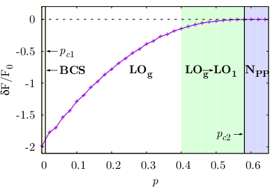
In Fig. 2 we present the $\text{LO}_{\text{g}}$ phase diagram in the canonical ensemble for polarizations, $p$, and for reduced temperature, $T/T_{F}=0$, and binding energy $\varepsilon_{B}=0.25\varepsilon_{F}$. For a fixed polarization $p$ we define the free Fermi gas Helmholtz free energy at zero temperature $F_{\text{free}}(T=0,n,p)$ and we introduce a rescaling constant $F_{0}=2\pi\times 10^{-2}\varepsilon_{F}N$, with $N$ the number of particles, such that we can plot the dimensionless quantity,

We see that the $\text{LO}_{\text{g}}$ phase is the energetically favorable ground state (with respect to the BCS and FF minima) for polarizations $0.02\leq p\leq 0.58$, above $p>0.58$ the system falls into the free Fermi gas phase ¹¹ 1 It is possible the ground state for these polarizations is the more complicated LO₂ phase, which is not considered in this work.. We know that a finite non-zero polarization destroys the BCS phase, and we see a transition at very low polarizations, $p_{c1}=0.02$. The finite nature of this transition is due to the numerical difficulty in finding the true ground state. We expect that for finite non-vanishing polarizations below the transition, $p<p_{c1}$, the $\text{LO}_{\text{g}}$ phase is still the ground state. At high polarizations $0.40<p<0.58$ the $\text{LO}_{\text{g}}$ and LO₁ phase have merged, and we will explore and elucidate this part of the phase diagram further below through the structure of the order parameter.

In Fig. 3 we explore the spatial distribution of the order parameter (solid line) and the local spin polarization (dashed line),

from the converged BdG solutions for polarizations $p=0.08$ (a), $p=0.10$ (b), and $p=0.28$ (c) as a function of the box length, $xk_{F}$, where $k_{F}$ is the Fermi momentum. We see in Figs. 3(a)-(c) that the increasing polarization, $p$, leads to a higher main amplitude, $Q$, and becomes consistent with the LO₁ ansatz. The local spin polarization is plotted as a function of space and we observe the structure imposed by the $\text{LO}_{\text{g}}$ phase. We see the favorable ground state configuration places the excess spin up atoms (the majority) where the order parameter vanishes, and the superfluid fraction at the peaks, and here excitations are less probable to occur, preserving superfluidity.

We can compare the $\text{LO}_{\text{g}}$ ground state order parameter with the LO₁ ansatz, by decomposing the self-consistently computed order parameter through a cosine Fourier transform. The order parameter has to be an even function along the chosen preferred direction, that is

then the $\text{LO}_{\text{g}}$ and the LO₁ are the same phase when the Fourier transform has only one mode.

In Fig. 4(a) we show that the self-consistent $\text{LO}_{\text{g}}$ phase is a superposition of different Fourier cosine modes and has a main mode occupation that is provided by the LO₁ ansatz. A comparison between the $\text{LO}_{\text{g}}$ phase configuration versus the LO₁ indicates that the $\text{LO}_{\text{g}}$ choice is always energetically favourable. This fact is true at both low and high polarizations where the $\text{LO}_{\text{g}}$ and LO₁ phases almost match. In order to explore this overlap we study the percentage occupation of the main mode and we observe in Fig. 4(b) that a perfect overlap between the phases never fully occurs. We can then conclude that there is always a combination of modes that is the energetically preferred ground state.

In Fig. 5 we show the behaviour of the Helmholtz free energy for two different cases, (a) at zero temperature and letting the polarization vary, while in (b) the polarization is fixed at $p=0.07$ and we increase the temperature. Figure 5(a) shows that the minimum of the free energy that occurs at $Q_{\text{min}}$ always lies away from $Q/k_{F}=0$ and $Q_{\text{min}}$ increases proportionally with the polarization. Figure. 5(b) shows that there is a transition point between the $\text{LO}_{\text{g}}$ phase and the BCS phase in the temperature range $0.15T_{F}<T<0.20T_{F}$. We observe that the increase of polarization pushes the minimum to high $Q$ values, while the increase of temperature pushes it back towards the $Q=0$ limit (i.e., the BCS phase). This behaviour is expected to change for high polarization when the $\text{LO}_{\text{g}}$ phase has a transition directly to the free Fermi gas phase. We note that the interaction strength $\varepsilon_{B}=0.25\varepsilon_{F}$ requires a pair-fluctuation treatment to produce quantitative results as the mean-field theory predicts the transition temperature from the BCS to normal state of $0.41T_{F}$, well above the experimental observations [37, 48].

Although the canonical ensemble can tell us about the properties and exotic phases of a spin polarized Fermi gas, it is important to know the nature of the phase transitions and the transition temperatures of the phases we have described so far; to perform this we will now work in the grand canonical ensemble. The absolute minimum of the thermodynamic potential is found at fixed chemical potentials, $\mu$ and $\delta\mu$, and this minimum moves through the landscape of the thermodynamic potential, giving us an insight as to the order of each phase transition. To explore the system we first need to study the behaviour of the the chemical potentials, $\mu$ and $\delta\mu$, found through the self-consistent BdG method in the canonical ensemble. We explore different regimes through the equations of state, $\mu(n,\delta n)$ and $\delta\mu(n,\delta n)$, with respect to a fixed density $n=k_{F}^{2}/(2\pi)$ and varying polarization to justify the regimes of interest in the grand canonical ensemble.

The values of $\mu$ and $\delta\mu$ used to compute the real order parameter, $\Delta(x)$, at fixed density $n$ and polarization $p$, normalized by Fermi energy and polarization multiplied by the Fermi energy respectively, are plotted in Fig. 6. The shaded regions correspond to the phases found in Fig. 2, at polarization $p_{c1}\simeq 0.02$, where we have the transition from BCS to $\text{LO}_{\text{g}}$, and $p_{c2}=0.58$, for the transition from $\text{LO}_{\text{g}}$ to N${}_{\text{PP}}$ ²² 2 The distinction between the fully polarized normal Fermi gas N_FP and the partially polarized N${}_{\text{PP}}$ that occurs when $\delta\mu>\mu$ is not taken into account here and we will use the notion of free Fermi gas for the N${}_{\text{PP}}$ phase. . At zero temperature, the BCS phase is favourable only at $p=0$. The underlying mean-field theory in 2D for the equation of state of a possible phase-separation phase (i.e., a mixture of a BCS superfluid and a normal gas) has been studied in Ref. [50] and the $\delta\mu$ versus $\mu$ phase diagram that involves the transition between BCS phase and the free Fermi gas has been explored therein. We take the salient results here,

The upper limit for $\delta\mu$ is the Clogston-Chandrasekhar (CC) limit,

above which the superfluid breaks down.

We observe that both $\mu$ and $\delta\mu$ assume an almost direct proportionality with the Fermi energy $\varepsilon_{F}$ and the polarization $p$ whenever $\delta\mu$ is large enough. Since in the grand canonical ensemble the $\text{LO}_{\text{g}}$ phase arises at high $\delta\mu$, we consider the case of $\mu/\varepsilon_{F}=1$ and vary $\delta\mu$ through the CC limit at different binding energies.

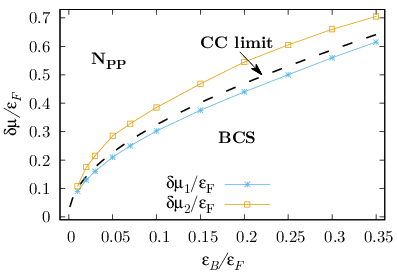
Taking the above values for the chemical potentials, in Fig. 7 we plot the phase diagram of the spin imbalanced Fermi gas, as a function of the binding energy, $\varepsilon_{B}/\varepsilon_{F}$, and dimensionalized chemical potential difference, $\delta\mu/\varepsilon_{F}$. The dashed line represents the CC limit, and we observe that the $\text{LO}_{\text{g}}$ phase provides two transition lines that we will denote with $\delta\mu_{1}$ (stars), below the CC limit, and $\delta\mu_{2}$ (squares), above it. In particular, the $\delta\mu_{2}$ line is in agreement with the results provided by the FF ansatz in Ref. [33]. It is interesting to observe how the reduced dimensionality of the problem, at least at zero temperature, enhances the effect of both the FF and the $\text{LO}_{\text{g}}$ phase. In 3D, it is possible to estimate that the FFLO phase is available for roughly 4% of the $\delta\mu$ values for which a superfluid phase is favourable, either BCS or FF, as evaluated from the phase diagram temperature versus magnetization [51]. We find from examining the corresponding region in Fig. 7 that, at a fixed binding energy, the FFLO is accessible for roughly 17% of the phase space, in which the system is a superfluid, that is, $(\delta\mu_{2}-\delta\mu_{1})/\delta\mu_{2}\simeq 0.17$.

We can find the favorability of the $\text{LO}_{\text{g}}$ phase compared to the BCS and FF phases by finding the absolute minima of the thermodynamic potential. In Fig. 8 we plot the local minima of the thermodynamic potential of three different ansatze, BCS, FF, and $\text{LO}_{\text{g}}$, for two binding energies, $\varepsilon_{B}=0.10\varepsilon_{F}$ (2) and $\varepsilon_{B}=0.25\varepsilon_{F}$ (1). Varying the dimensionless chemical potential difference, $\delta\mu/\Delta_{0}$, where $\Delta_{0}$ is the BCS order parameter at zero temperature, we determine the region where the $\text{LO}_{\text{g}}$ phase is favorable. The intersection of different phases determines the critical values $\delta\mu_{1}$ (i.e., from the BCS to $\text{LO}_{\text{g}}$ transition) and $\delta\mu_{2}$ (i.e., from the $\text{LO}_{\text{g}}$ to $\text{N}_{\text{PP}}$ transition).

We see in Fig. 8 that the $\text{LO}_{\text{g}}$ to $\text{N}_{\text{PP}}$ transition is smooth ³³ 3 The FF line of minima is always above the $\text{LO}_{\text{g}}$ line close to the BCS line, although at high $\delta\mu$ values, the model accuracy doesn’t allow us to conclude whether there is, or isn’t, another transition FF-$\text{LO}_{\text{g}}$. Besides, we must say that is very inessential because, at high $\delta\mu$, the energy gap parameter reduces continuously its amplitude until it vanishes and the difference between the magnitude of the two ansatze might be neglegible. Moreover, at high $\delta\mu$ values it’s even more likely, as discussed in Section II, the presence of an LO₂ phase. The latter might actually be favourable with respect to both FF and $\text{LO}_{\text{g}}$. while the BCS to $\text{LO}_{\text{g}}$ has a discontinuity, although not easy to observe. The order of the BCS-$\text{LO}_{\text{g}}$ transition can be examined as we increase the binding energy $\varepsilon_{B}$. We check the behaviour of the order of phase transitions in Fig. 9, where we have plotted the thermodynamic potential of the $\text{LO}_{\text{g}}$ phase as a function of $Q$ at the points labelled (a)-(d) in Fig. 8 for the interaction strength $\varepsilon_{B}=0.10\varepsilon_{F}$, sliced at different $\delta\mu$ values. The comparison between subplots Fig. 9(c) and (d) reveals the second order nature of the $\text{LO}_{\text{g}}$-$\text{N}_{\text{PP}}$ phase transition. In this part of the phase diagram, an increase of $\delta\mu$ leads to: (i) an increase of the LO momentum $Q$, (ii) the order parameter amplitude squeezes until it vanishes in $\delta\mu_{2}$ and (iii) the order parameter frequency matches the LO₁ initial ansatz. The BCS-$\text{LO}_{\text{g}}$ phase transition can be studied by observing the evolution of the thermodynamic potential in the subplots Fig. 9(a) and (b). It is known that the FF phase undergoes a first order phase transition towards the BCS phase [33]. In our case, the presence of a local maximum at small $Q$ in the subplot Fig. 9(a) is an indication of the first order phase transition. However, within our accuracy, the local maximum is shown by a single point only. It is possible to increase the binding energy, and thereby to relatively improve the accuracy of the calculation. As shown in Fig. 9(e), at $\varepsilon_{B}=0.35\varepsilon_{F}$, the local maximum at low $Q$ becomes more evident. Considering the accuracy of our numerical calculations and also the difficulty of reaching convergence close to the BCS-$\text{LO}_{\text{g}}$ transition line, we cannot make a conclusive determination of the order of the BCS-$\text{LO}_{\text{g}}$ transition. Throughout the work, we interpret it as a weak first-order transition, to reflect the fact that the strucuture of the local maxiumum is weak.

We can extend the BdG equations from the zero temperature regime to study the $\text{LO}_{\text{g}}$ phase at finite temperatures. In the deep BCS limit the critical transition temperature, $T^{\text{BCS}}_{c}$, can be approximated from the gap equation in 2D following Landau theory of the second order phase transition,

where $\gamma$ is the Euler-Mascheroni constant. We can estimate the tricritical point (TCP) temperature, where the BCS, CC limit and FFLO phase intersect, with the numerical value [53, 54, 55]

From our self-consistent BdG equations we plot out the phase diagram for the critical temperature as a function of chemical potential difference in Fig. 10 for interaction strengths (a) $\varepsilon_{B}=0.10\varepsilon_{F}$ and (b) $\varepsilon_{B}=0.25\varepsilon_{F}$, the inset shows the entire phase diagram. The transition between the BCS and $\text{N}_{\text{PP}}$ phase, found through the BCS theory, is second-order for temperatures above $T_{\text{TCP}}$. The first-order CC limit (dashed line) is entirely contained in between the two $\text{LO}_{\text{g}}$ transition temperatures at any relevant $\delta\mu$ value. Moreover, the order of the phase transitions is preserved, the second order phase transition between the $\text{LO}_{\text{g}}$ and $\text{N}_{\text{PP}}$ phase is unaffected by an increasing temperature below TCP. The weak first-order BCS-$\text{LO}_{\text{g}}$ is preserved within our numerical accuracy.

We note that, in the weakly-interacting regime $\varepsilon_{B}=0.10\varepsilon_{F}$, $T_{c}^{\text{BCS}}$ is approximately $0.25T_{F}$. It appears that the mean field treatment requires a beyond mean-field approach to take into account the fact there is no superfluid behaviour above the Berezinskii-€“Kosterlitz-€“Thouless (BKT) temperature $T_{\text{BKT}}\simeq 0.125T_{F}$. We observe that most of the $\text{LO}_{\text{g}}$ phase is below $T_{\rm BKT}$, and within our numerical calculations the existence and availability of the $\text{LO}_{\text{g}}$ phase at finite temperatures is also below the TCP temperature, at least in the weakly-interacting regime. However, we cannot provide accurate quantitative results for the transition temperatures among the phases under investigation due to the mean-field nature of the calculation.