Convergence of dual ascent in non-convex/non-differentiable optimization
Abstract
We revisit the classical dual ascent algorithm for minimization of convex functionals in the presence of linear constraints, and give convergence results which apply even for non-convex functionals. We describe limit points in terms of the convex envelope. We also introduce a new augmented version, which is shown to have superior convergence properties, and provide new results even for convex but non-differentiable objective functionals (as well as non-convex).
The results are applied to low rank approximation of a given matrix, subject to linear constraints. In particular, letting the linear constraints enforce Hankel structure of the respective matrices, the algorithms can be applied to complex frequency estimation. We provide numerical tests in this setting.
1 Introduction and Motivation
A classical algorithm for solving linearily constrained convex optimization problems is the dual ascent scheme. Given a functional on some Hilbert space and a set of linear constraints , where is a linear operator, the objective is to solve
| (1) |
For simplicity we assume that since this can be achieved by translating the origin. The condition then becomes equivalent to where is the kernel of .
The dual ascent method considers the dual problem where the dual function is and the Lagrangian is
| (2) |
The parameter is the so called Lagrange multiplier and is an element in the codomain of . By introducing we may equivalently consider the restricted Lagrangian
| (3) |
The dual ascent method tries to maximize the dual function by alternatively updating and according to
| (4) |
where denotes projection onto . It can be seen that is a subgradient of at (see Section 2 for details), and the -update can therefore be thought of as a projected gradient ascent step.
The main objective of this paper is to derive convergence results for cases where the objective function is non-differentiable and non-convex. While there exist general convergence results for the dual ascent approach these typically make additional smoothness assumptions (see Section 1.2). In contrast, the non-differentiable case remains relatively unexplored. Our work is motivated by the problem of least squares low rank approximation with constraints. Here
| (5) |
where is a rank penalizing parameter, is a fixed matrix, typically related to measured data, and denotes the Frobenius norm. The constraint set corresponds to some specific matrix structure, such as Hankel-form. Note that the -function is constant everywhere except on a set of measure zero and non-convex. Furthermore, the sought optimum is typically of low rank and therefore located in the vicinity of discontinuities. This article contains convergence results that applies to the dual ascent scheme (4) in this situation, distinguishing it from previous contributions listed in Section 1.2.
1.1 Contributions and Results
The main contributions of our paper are twofold:
- •
We show convergence of the dual ascent updates (4) for a general class non-convex (possibly discontinuous) objective functions and describe the limit point in terms of the lower semi-continuous (l.s.c) convex envelope of denoted .
- •
We propose a family of augmented formulations that can approximate the original problem arbitrarily well while exhibiting improved convergence properties. This also gives new results about convergence for non-differentiable convex functionals.
Our results are valid under the assumption of a so called feasible objective (see Definition 3.1 for details). The functions is feasible if it is l.s.c, proper and grows sufficiently fast as .
Theorem 1.1.
Let be feasible and consider the dual ascent scheme
| (6) | ||||
| (7) |
with . Suppose that the sequences and are bounded. Then there are convergent subsequences of and with corresponding limits and satisfying; If , then it is a solution to
| (8) |
Moreover this happens whenever
has a unique solution.
We remark that may be replaced by more general sequences, see Theorem 4.1 for more details.
The condition on boundedness clearly limits the applicability of the above result, but we will show that these are satisfied in the situation of low-rank approximation (Section 6). Moreover it would be desirable for the entire sequence to converge. The next theorem show that these issues disappear upon adding a small quadratic term to the objective functional.
Theorem 1.2.
Let be fixed, let be a finite-valued feasible functional, and consider the augmented dual ascent scheme
| (9) | ||||
| (10) |
with . It then holds that and converges to some limits and , where is the solution to
| (11) |
In fact, if is convex to begin with, but non-differentiable, then and the above result is new even in this case.
Note that in contrast to our formulation (9), standard augmentation approaches [8] typically add the penalty term , which results in the augmented Lagrangian
| (12) |
The above expression is convex for a fixed . However, in the context of low rank approximation, where is an -matrix, becomes an -matrix and the corresponding minimization over becomes very slow. In contrast, the update of (9) has a closed form expression (in terms of the singular value decomposition) allowing rapid computation. The price one has to pay for this is that the affects the functional on the subspace , albeit negligibly assuming that is small.
Theorem 1.2 is a combination of Theorem 5.1 and its corollaries. The full version also includes -valued functionals. Moreover, Corollary 5.3 provides information on the speed of convergence of . To compute the update (9), explicit knowledge of is needed, which is convex (but not necessarily differentiable). However, the (non-convex) updates (6) clearly arise as the limiting case of (9) as so when is known the augmented scheme (9)-(10) can be viewed as a minor modification of the original (6)-(7), except for that the step-length in 10 is fixed. In section 5.1 we present a crossover algorithm where this constraint is lifted, which in our numerical section 7 is shown to have superior performance.
In Section 6 we consider the objective function (5). We give explicit expressions for the convex envelope as well as formulas for the corresponding updates (6)-(7) (Proposition 6.2) and (9)-(10) (Proposition 6.1). Concerning dual ascent, we prove that the sequences and always are bounded, so that Theorem 1.1 applies (see Theorem 6.3). Concerning augmented dual ascent, Theorem 1.2 applies as stated above and yields that we always find a convergent sequence whose limit point solves (11) (see Theorem 6.5).
1.2 Related work
The dual ascent algorithm goes back to the 60’s [16], and the augmented version as well [20], although other precursors relying on Lagrange multipliers are sometimes mentioned. We refer to [10] or [8] for a more thorough overview of early results. Chapter 2 of the latter reference is devoted to the minimization of a non-convex functional under the constraint , using dual ascent schemes similar to (6)-(7) and (9)-(10), relying on Lagrangians of the type (3), but only local convergence results are provided, assuming that one starts near a minima with positive Hessian. As noted in Section 1 dual ascent is in fact a special case of the projected subgradient method, see e.g. [9], Section 4.2 of [7] or Chapter 6 (available online only) of [6], for introduction and recent convergence results.
In the 90’s these methods were extensively studied by Luo and Tseng [29, 28, 36], mainly focusing on the convex situation and convergence under various smoothness assumptions on . They also began to study coordinate splitting methods [27], a work that was subsequently extended also to non-convex functionals [37], albeit working with weaker concepts of convexity such as pseudoconvexity, quasiconvexity, hemivariate. A more recent contribution in this direction is [19], which considers convergence of ADMM in the convex setting, a work that has inspired the proof of Theorem 1.2.
There is a large body of work dealing with low rank approximation and optimization. One of the earliest results is the Eckart-Young-Schmidt theorem [34, 15] which gives a closed-form solution for the best least squares approximation of a given matrix with a matrix of specified maximal rank. More precisely, given a singular value decomposition (SVD) of the best rank- approximation can be found by setting all but the first singular values to . In many applications (e.g. [30] and the references therein) it is of interest to add additional constraints and penalties that model any additional prior knowledge we may have about the solution. Adding any convex constraint to the formulation may seem like a minor change, however since the original formulation is not convex this makes the problem much more complicated and in practice iterative approaches (see e.g. [26]) without optimality guarantees have to be applied.
In order to develop more flexible methods that allow incorporation of application specific priors researches have started to consider convex formulations for rank approximation. A popular heuristic is to replace the rank function with the so called nuclear norm [32, 13, 31, 3]. Since this formulation penalizes all the singular values, not just the small ones, it has a shrinkage bias making it sensitive to high levels of noise and missing data (e.g. [25, 31]).
The original motivation for using the nuclear norm was given in [17] where it is shown that the nuclear norm is the convex envelope of the rank function on the set , where is the largest singular value of . The constraint is artificial and added since the convex envelope on the whole domain would simply be the zero function. Very recently it has been observed [25, 23] that a significantly stronger relaxation can be derived if one considers, not just the rank function, but also a least squares penalty term . The penalty term, which replaces the constraint, effectively restricts the feasible domain to a neighborhood around . As a consequence the obtained envelope, see (52), is much more accurate in this region. In contrast to the nuclear norm it does not penalize singular values larger than and therefore does not exhibit the same shrinking bias.
Because of the difficulty of achieving guaranteed global optimality local approaches are often employed. If the rank of the sought matrix is known, bilinear parameterizations where the matrix is factored into are used. The easiest approach is to alternatively reestimate and , e.g. [30]. Buchanan and Fitzgibbon [12] showed that this method often exhibit very slow convergence. Instead they proposed a damped gauss-newton update that jointly optimizes over both factors. Hong and Fitzgibbon [21] provide a unified theoretical framework and experimental comparisons of many of these local factorization methods with least squares residuals.
Finally, for the particular case of Hankel matrices and frequency estimation, the problem is severely non-convex with many local minima near the (constrained) global minima, see e.g. Figure 1 in [26] and the surrounding discussion, or Section 3 in [18]. To deal with this situation [26, 18] propose to also iterate over the initial guess. Section 4 of the (recent) article [18] also contain a brief discussion of state of the art methods for the Hankel low rank approximation problem (sometimes called Hankel SLRA), where it is stated that “None of these methods have the theoretical property of convergence though and hence the construction of reliable methods for solving the Hankel SLRA problem remains a wide open problem.”
2 Preliminaries
In the entire paper will denote a finite dimensional Hilbert space. By a proper fuctional we mean a valued function on which is not identically equal to . Let be a convex lower semi-continuous (l.s.c.) proper functional on . The subdifferential of is denoted and consists of all that fulfill
| (13) |
for all . Similarly, in the concave case the subdifferential consists of all fulfilling the opposite inequality. A vector in is denoted . By we mean the Fenchel conjugate
| (14) |
(since there is no risk of confusion, we use this notation also for adjoints). Note that the double Fenchel conjugate is the l.s.c. convex envelope of (see e.g. Proposition 13.39 [5]).
Let be a closed linear subspace and consider the problem
| (15) |
Introduce an orthonormal basis for , and similarly an orthonormal basis for . If is the operator whose output is the coefficients of in the basis , then (15) can be written as
| (16) |
(in fact, any operator with would do). Following the method of multipliers (see e.g. [9], Chapter 6 and 7), we introduce the Lagrangian
where is the so called Lagrange multiplier and the scalar product is the canonical one in . Since , and , we may equivalently consider the restricted Lagrangian
| (17) |
where replaces . The dual function is then
| (18) |
In particular, is concave. The dual ascent consists in applying the projected subgradient method to the function and the subset , (see [10] Section 2.1 and [9], Chapter 6 and 7). More precisely, if we let denote the projection of onto the subspace , i.e. , then the dual ascent algorithm for (16) reads
| (19) |
for some sequence of predetermined parameters , (see e.g. Ch. 6 and 7 in [9]), and . To better see the connection between the updates and the subgradient of , we remind the reader that
| (20) |
(see e.g. [5], Theorem 16.23). In terms of and , (20) reads
| (21) |
Since clearly in (19), it follows that and hence the update for can be rewritten
The iterates thus ascend on the concave hill , at least if the step length is not too big.
3 Non-convex cost functionals
Suppose now that is a non-convex proper l.s.c. functional that we wish to minimize over some subspace of the finite dimensional Hilbert space . One may then still attempt the dual ascent minimization scheme,
| (22) | ||||
| (23) |
albeit with little hope of being able to prove convergence or, in case it converges, proving that we have found a global minimum.
Since (see e.g. Prop. 13.14 in [5]) we have
| (24) |
That is, the dual functions obtained using and its convex envelope respectively, coincide. Furthermore, it is a simple observation that
| (25) |
Hence the sequence generated by (22)-(23) is contained among the sequences that can be generated by a dual ascent scheme using . This makes it plausible that it should in fact converge to an optimum of .
While and typically attain the same minimal values it is important to realize that if we restrict the functionals to this may no longer hold. The convex envelope over , i.e. , does not necessarily coincide with restricted to , (i.e. ), see Figure 1. The latter is clearly a convex function which lies below , so we do have
We will give conditions under which the dual ascent scheme (22)-(23) converges, and show that the convergence point is then typically a solution of . Note that computing is just as difficult as solving the original non-convex problem since
| (26) |
and therefore not feasible to work with.
3.1 Feasible functionals
In order for the above discussion to make sense, we have to assume that grows fast enough in all directions so that the above minimizers exist. We therefore restrict attention to the following class of functions, (in the notation of [5], functionals that satisfy (27) are called supercoercive);
Definition 3.1.
A l.s.c. proper functional will be called feasible if it is bounded below and
| (27) |


In the remaining part of this section we establish some results concerning feasibility of conjugate and double conjugate functions that will be useful later on. The next proposition summarize properties of .
Proposition 3.2.
If is feasible then is a continuous convex functional which is bounded below. Furthermore, both and its subdifferentials are bounded on bounded subsets of . Finally, if is finite-valued, then is feasible. In particular it then has bounded level sets.
Proof.
That is bounded below follows by the trivial estimate for all . We now consider bounds from above.
Given set , which by assumption is bounded below and satisfies . Fix and suppose that satisfies . Then
Since the second term of the product will be negative for sufficiently large , the supremum is clearly finite and independent of (as long as ), so is bounded on bounded subsets of . That is convex is well-known and easy to check, (see e.g. Proposition 13.11 in [5]). Since a locally bounded convex function is continuous ( Corollary 8.30 in [5]) it follows that is continuous. Theorem 16.17 in the same reference also yields the statement concerning subdifferentials.
Now let be finite-valued and suppose that is not supercoercive. Pick a sequence such that
and . Since the unit ball is compact in finite dimensional Hilbert spaces, there exists a subsequence such that converges to some with . By the Fenchel-Young inequality (Proposition 13.13 [5]), we then have
which is a contradiction. ∎
The bounded level sets of will be an important condition in subsequent results, and it is therefore important to realize that this property may fail even in the convex case, if assumes the value Pick for example and
for which
In the next proposition we collect properties of .
Proposition 3.3.
If is feasible, then so is .
Proof.
is l.s.c since it is the Fenchel conjugate of . As already noted, is the l.s.c. convex envelope of , and hence it is bounded below since is, and proper since . To show that satisfies (27), let be arbitrary and pick such that whenever . Let be a bound from below for and note that
Since the right hand side side is a convex lower bound on it follows that
from which the desired conclusion is immediate, as was arbitrary. ∎
4 Convergence of dual ascent
Let be a non-convex proper l.s.c. functional on some (finite dimensional) Hilbert space , that we wish to minimize over a subspace . In this section we provide a general convergence result for the dual ascent scheme (22)-(23). This result only gives convergence of a subsequence, which can be remedied by considering an augmented variation of the algorithm. This is done in Section 5.
Theorem 4.1.
Proof.
As noted in Section 3, the updates are the same as if we apply dual ascent to the convex l.s.c. functional , (recall (19)). Note that (see e.g. Prop. 13.14 in [5]), so that the dual function introduced in (18) becomes
| (32) |
Note that the sequence is non-decreasing by the definition of the numbers . As we observed in Section 2, the updates for are those one gets by applying the projected subgradient method to and . Since is a bounded sequence and has uniformly bounded subdifferentials in any ball of a fixed radius (Proposition 3.2), it follows by the results in [9] (see in particular equation (2)), that converges to the maximum value of , as long as satisfies the stated conditions.
Since and are bounded sequences they have convergent subsequences (by Alaoglu’s theorem). Let be any strictly increasing sequence such that both and converge, and denote the corresponding limits by and . By Proposition 3.2 is continuous and therefore is the maximum of . We also claim that
| (33) |
which clearly follows if we show that . This in turn is clear by the identity , which holds for all , and the continuity of .
The minimum of
| (34) |
is attained for some on , for otherwise standard arguments show that a different value of would yield a higher value of (see e.g. Sections 5.2.3 and 5.4.2 in [11]). By definition this minimum equals and since it follows that
where the last identity follows by (33). With this we have established (30).
The above chain of equalities also implies
so if (34) only has one minimizer we immediately deduce that , and the remainder of the theorem follows. ∎


| 0 | - | 0 |
| 1 | 1 | 1 |
| 2 | -1 | 1/2 |
| 3 | 1 | 1/6 |
| 4 | -1 | -1/12 |
| 5 | 1 | 7/60 |
When (31) does not have a unique solution there may not be any subsequence that converges to an . As an example, consider the case of , , and . Then so . It is easily computed that for , and elsewhere. Clearly . The functions , and are displayed in Figure 2 together with a sequence generated by dual ascent for this problem. It is clear that will oscillate between values in whereas . Thus, depending on which subsequence is chosen, will be either 1 or -1, and in neither case does it lie on . To avoid the possibility of such undesirable sequences, we now consider an augmented version.
5 Convergence of augmented dual ascent
In this section we will make a minor change of the algorithm and give a different proof, inspired by [19], leading us to assume instead that is fixed. We first consider the case when is a convex feasible functional on some (finite dimensional) Hilbert space and a subspace, and discuss the important particular case in Section 5.2. We introduce the augmented dual ascent scheme
| (35) | ||||
| (36) |
with . To our best knowledge the following result, which assumes no differentiability of , is new.
Theorem 5.1.
Let be fixed and let be a convex feasible functional. Suppose that , given by (36), is a bounded sequence. It then holds that and converges to some limits and , where is the solution to
| (37) |
Remark; the condition on is fulfilled whenever is finite-valued, see the corollaries.
Proof.
Set , let be as in Section 2 and define by
| (38) |
Since is feasible it directly follows that is feasible. Proposition 3.2 thus implies that is bounded below which implies that is bounded above. Also note that, since the sequence lies in by definition, see (36), there is no difference between and for these points. Clearly
| (39) |
and from (21) we know that if and only if . Note that is given by
i.e.
and hence we conclude that
| (40) |
Combining (36) and (39), we see that (40) implies the following;
| (41) |
where is arbitrary. Setting immediately gives
| (42) |
so increases for each iteration. Thus exists, and since is bounded above it is finite. We now show that this is actually the supremum of . First note that
| (43) |
If is a point such that , then the above is positive by (41), which means that is decreasing with increasing . Moreover, combining (41) with (43) we get that the (positive) sum
is bounded by , which shows that . By recalling that this also equals , it follows that can not hold for any point. We conclude that is indeed the supremum of .
Since is a bounded sequence (and is finite dimensional) it has a convergent subsequence , whose limit we denote by . By (38) and the fact that is l.s.c, it follows that is u.s.c. and so , so . Let in (41). Fix and let be a number in the subsequence such that . Similarly to above we then have
| (44) |
which in the limit gives
Both sums are convergent since their summands are positive. It follows that we can make arbitrarily small upon choosing sufficiently large, (and also that this quantity is decreasing). It follows that , as desired.
It remains to prove that converges to a minimum of (49). The operator which is implicitly defined in (35) (taking to ) equals the proximal mapping of evaluated at Since is convex and l.s.c., these mappings are firmly non-expansive, and in particular continuous (see e.g. Ch. 4.1 and 12.4 in [5], in particular Proposition 12.27). The convergence of thus follows from that of . Finally, if would not be a solution to (49), then we can argue as in the end of Theorem 4.1 to get a contradiction (see (34) and use , which has a unique minimizer since it is strictly convex). ∎
We collect a few results that came out in the above proof.
Corollary 5.2.
Let , defined as in the above proof, attain its supremum. Then , given by (36), is a bounded sequence. In particular, this happens if is a feasible finite-valued functional.
Remark; the functional on given by for , and has and is convex (since it equals ). By modification of this simple example, one can show that there are situations where does not attain its supremum.
Proof.
The first part of the corollary follows immediately by the sentence following (43). If we now assume that is finite valued then so is , and Proposition 3.2 implies that is feasible. By (38) we conclude that attains its supremum.
∎
We now consider the speed of convergence of the dual variable.
Corollary 5.3.
Suppose that is bounded. Then is Fejér monotone with respect to the set of maximizers of , which is non-empty. Moreover, if is the supremum of then .
Proof.
The existence of maximizers was established in the proof of Theorem 5.1. Let be one such. It follows from (43) and the subsequent argument that is decreasing, i.e. that is Fejér monotone with respect to the set of maximizers of . Now recall that increases by (42). In analogy with (44) we can get the concrete estimate
showing that
Since is arbitrary and as , the limsup is actually 0, and hence the speed of convergence of is at least . ∎
5.1 Other steplengths
The augmented dual ascent scheme has a drawback; the term is included for convergence purposes and will influence the optimal point, and hence it is desirable to keep small. However, is also the step length in the updates of , and in order for the algorithm to converge rapidly one would like to have fairly large. To remedy this one may consider the following scheme
| (45) | ||||
| (46) |
where , which is closer to the original scheme (22)-(23). Upon assuming further regularity of , it is possible to modify the proof of Theorem 5.1 and derive conditions under which this scheme converges to
but we refrain from this and content with noting that the results of the previous section applies whenever for all sufficiently large (which is immediate by Theorem 5.1). We will however use the scheme (45)-(46) in our numerical section.
5.2 The case
We now move back to considering a non-convex feasible functional , as in Section 4. In this section we consider the augmented dual ascent scheme
| (47) | ||||
| (48) |
with , which is an alteration of (22)-(23). As we shall see, the addition of the quadratic penalty may alter the limit point slightly. However, for small values of it will give a good approximation. (In the context of low rank approximation we investigate this further in Section 7.) The penalty term allows us to prove convergence of the generated sequence itself without the need for examining sub-sequences. However, note that it does require explicit knowledge of .
Theorem 5.4.
Let be fixed and let be a feasible functional on some finite dimensional Hilbert space . Suppose that that is finite-valued, or that , given by (36), is a bounded sequence. It then holds that and converges to some limits and , where is the solution to
| (49) |
6 Low rank approximation with constraints
We now depart from the general theory and consider the problem of low rank approximation with subspace constraints where the objective function is of the form
| (50) |
where is an matrix.
Before we address the optimization schemes we present some useful results. For the above formulation (50) the conjugate function and the convex envelope can be computed in closed form [24]. The conjugate function is given by
| (51) |
and the convex envelope is given by
| (52) |
In the primal update of augmented dual ascent (47) we need to solve problems of the form
| (53) |
It turns out that this can be efficiently computed by modifying the singular values of . More precisely, suppose that has the singular value decomposition , where is a diagonal matrix containing the singular values . Given a function , we introduce the operator
| (54) |
that modifies by changing the singular values from to . This operation is known as the “singular value functional calculus” [2] as well as “generalized matrix function” [4]. The following proposition now shows how to solve (53).
Proposition 6.1.
Proof.
By von-Neumann’s inequality both problems are solved by a matrix of the form , (for a detailed version of this inequality, which also provides the above information on the singular vectors at optimum, see e.g. [14]). Therefore the singular values are found by minimizing
Differentiation of this expression shows that the minimum given by . ∎
Note that for the objective is strictly convex and the minimum is therefore unique. The next proposition characterizes all the solutions for the case .
Proposition 6.2.
Proof.
Again, von-Neumann’s inequality implies that both problems are solved by a matrix of the form . To chose the ’s in the case of , we need to minimize the functional
and it is easy to see that the solutions are as stated in (55). The corresponding statement for is even simpler, we omit the details. The final statement is obtained by setting whenever there is ambiguity, i.e. . ∎
Figure 3 shows examples of when for different values of alpha. Note that in all cases will set singular values less than to zero. For singular values larger than remain unaffected by , while for these are subjected to a penalty. We also remark that the so called "hard thresholding" performend by gives a minimizer of both and although it may not be unique in either case.

6.1 Dual ascent
The dual ascent algorithm (22)-(23) for trying to minimize (50) reads
| (56) |
The Lagrange multiplier can easily be absorbed into the quadratic term, since
| (57) |
and is independent of . Using (57), the scheme becomes;
| (58) |
with . By the remarks in Section 3 (as well as Proposition 6.2), it is also a dual ascent scheme for the minimization of over .
Similar to Section 4 we let
| (59) |
Theorem 6.3.
Proof.
It is clear that is feasible so Theorem 4.1 applies. The fact that both sequences and are bounded is shown separately in Proposition 6.4 below. Assuming this, Alaoglu’s theorem implies that both sequences and have convergent subsequences. For the final statement, it follows by (57) that
and hence Theorem 4.1 and Proposition 6.2 together imply that the corresponding minimization problem has a unique solution if and only if has no singular value equal to .
∎
Proposition 6.4.
If for all , then the sequences and given by (58), are bounded.
Proof.
The sequence is clearly bounded if is. To prove that is bounded, first note that
| (60) |
Since and is self-adjoint, we also have
The operator keeps only the singular values lower than , and sets the other ones to 0. Thus , where is the amount of singular values. Setting , the Cauchy-Schwartz inequality thus gives
| (61) |
Moreover, since both and are contractions we have
| (62) |
Combining (60)-(62) and recalling that , we get
where and . Note that these constants are independent of . Setting our inequality can be written
Whenever we clearly have . Now suppose that is not negative everywhere. Then it has two real roots, and takes positive values between them. Let us denote the larger root by and the maximal value by . Recall that . For the quantity can now be uniformly bounded by the constant , and for the earlier inequality reads . Summing up, we have shown that
from which it clearly follows that is a bounded sequence. ∎
6.2 Augmented dual ascent
By (57) and Proposition 6.1 it follows that the augmented dual ascent scheme (47)-(48) takes the form
| (63) |
with . Note that the primal update of the (un-augmented) dual ascent scheme (58) is the limiting case as , which has been claimed earlier in the paper. Theorem 5.1 and Corollary 5.2 immediately gives
Theorem 6.5.
The sequences and converge to some limits and , where is the solution to
| (64) |
7 Numerical Evaluation
In this section we evaluate the proposed methods in the context of rank minimization with Hankel constraints. An example of an application is the decomposition of a signal into complex exponentials. There is a well known connection between the rank of a Hankel matrix and the number of exponentials needed for the generating function of the Hankel matrix, usually referred to as Kronecker’s theorem [22]; Given a complex valued vector with elements
| (65) |
the Hankel matrix generated by the vector (i.e., the elements of satisfy ) is of rank (with the exception of degenerate cases), and conversely, if a Hankel matrix has rank then its generating vector is of the form (65) (again with the exception of degenerate cases), see [1].
7.1 Convergence Evaluation
We first perform a quantitative evaluation of the convergence of our algorithms. We compare three approaches:
- DA
-
- The dual ascent scheme (58) with the step-sizes .
- ADA
-
- The augmented dual ascent scheme (63) with a step-size .
- mod-ADA
To create low rank Hankel matrices we make use of Kronecker’s theorem and randomly select sums of exponentials. For the results displayed in Figure 4 we used
| (66) |
where and are uniformly distributed over and and belong to a normal distribution with mean zero and standard-deviation one. We sampled the function in equally spaced points between and and formed a Hankel matrix. Since each term in the sum (66) consists of two complex exponentials the resulting matrix, which we use as ground truth, will have rank 8. To generate the measurement matrix we added Gaussian noise with standard-deviation to each element of the ground truth matrix.
Figure 4 illustrates the convergence of the three methods. Here we solved instances of the problem and plotted average primal and dual objective values for the first iterations. In each iteration we generated a primal feasible solution by projecting the current estimate onto the closest Hankel matrix . To compute primal objective values we then used for DA and for both ADA and mod-ADA, since this is what the methods will converge to.
To evaluate dual objectives we used conjugates of the above primal functions. For DA the dual is simply with as in (51). For ADA and mod-ADA the conjugate can be computed by noting that
Inserting and maximizing the right hand side with respect to shows that optimal. Therefore we get the dual objective function
In Figure 4 we ran the experiment twice, first with and then with . For the methods seem to converge relatively fast (see Figure 4, left). For (Figure 4, right) the convergence of ADA becomes prohibitively slow since it is forced to very take small gradient steps. In contrast the variable step-size of mod-ADA still generates good solutions in very few iterations.


In Figures 6 and 6 we show the 10 leading singular values of the solutions given by the tree methods (averaged over all trials). For comparison we have also plotted the singular values of the measurement matrix and the ground truth (which is of rank ). While convergence of ADA is relatively fast for the added regularization term will penalize the larges singular values. For ADA and mod-ADA this results in the weak shrinking bias visible in Figure 6. For , see Figure 6, this bias is negligible but the slow convergence of ADA hinders the suppression of the small singular values. Hence for ADA there is a trade-off between accuracy and speed of convergence. The same tendency can be observed in Table 1 where we show the normalized distance to the ground truth, that is , if is the ground truth, averaged over all trials.
| DA | ADA | mod-ADA | |
|---|---|---|---|
| 0.1 | 0.0053 | 0.0479 | 0.0479 |
| 0.001 | 0.0050 | 0.0753 | 0.0049 |
According to the theory of Section 6.1 it may be necessary to select a subsequence to get convergence of DA. In Figure 7 we highlight a single problem instance (extracted from the experiment above) where the variables did not seem to converge for DA. To the left we plot the primal and dual objective values and to the right we plot the distance between the primal solution and the ground truth during 300 iterations. The dual variable exhibits a similar behavior as , note however that the dual objective values seem to converge nicely. For comparison we also plot mod-ADA which does not exhibit the same behavior.
The exact reason for this behavior is unclear but it seems to happen for difficult problem instances, when the size of the 8th (true) singular value is at same level as of the noise. Note that when using (66) this may happen if for example is close to zero. However the effects are not visible in Figure 4 due to averaging.


7.2 Performance in signal frequency estimation
In this section we compare our formulation to state-of-the-art frequency estimation methods. Kroeneker’s theorem is the basis for many of these methods such as for instance ESPRIT [33] and MUSIC [35].
We are interested in approximating a signal with a linear combination of exponentials. We use the formulation
| (67) |
where is a parameter that penalizes the number of exponential functions used in the approximation. Note that due to the Hankel structure, the Frobenius norm formulation above is equivalent (except some degenerate cases) to the weighted least squares objective
where is the triangle weight
This weight is undesirable, assuming that all signal samples are subjected to independent Gaussian noise, however removing it by modifying the Forbenius norm term makes primal updates much more difficult. Note that in contrast ESPRIT uses the unweighted least squares formulation, but without optimality guarantees.
5924.0i +1.00000+i0.00000 804.24i +0.62348+i0.78183 695.88i -0.22252+i0.97493 7937.6i -0.90097+i0.43388
We conduct experiments on a function of the form (65) with frequencies and coefficients given in Table 2. The function is sampled at 257 points, and white noise is added to achieve different signal-to-noise rations (SNR). In the simulations below we tested SNR levels between 0 dBW and 25 dBW in steps of 2.5 dBW. For each SNR level 10000 simulations where computed using the dual ascent method and the ESPRIT method. For the ESPRIT approach, exponentials are estimated using the largest singular vectors, and a least squares fit is used to determine the coefficients in (65). A Hankel matrix is then generated from this vector and the approximation error is computed in Frobenius norm. For the dual ascent method, the penalty level is chosen as , where is the Hankel matrix from the noisy signal. The stepsize parameters are chosen so that they decay as , and the algorithm is stopped when .
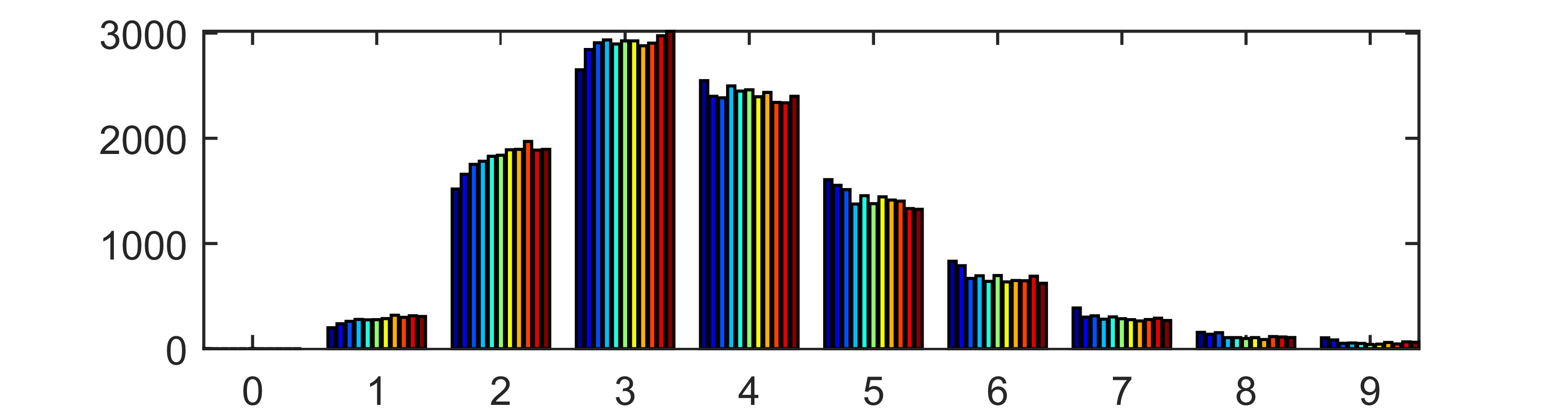
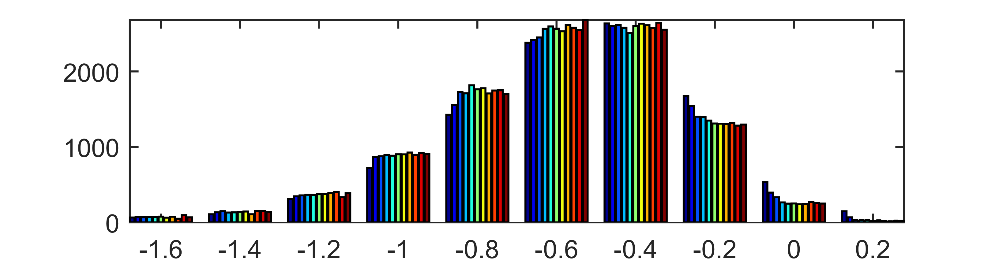
In the top left panel of Figure 8, the difference between the Frobenius errors obtained by the ESPRIT method and the dual ascent method are shown in bar plots. The differences between the errors are scaled with the noise level in order to illustrate them in the same plot, i.e., the bar plots illustrates
From Figure 8 there are very few events on the lowest bar group, i.e., when the errors between the two methods are of equal size. In fact, the error obtained by the ESPRIT is higher than the one obtained by the dual ascent in every single one of the 110000 simulations. Note though that this result holds with respect to error in the Frobenius norm and not in the regular -norm for the vectors. The lower left barplot of Figure 8 shows the difference in norm on the vectors that generate the Hankel matrices, i.e.,
where and are the vectors that generate the Hankel matrices and , respectively. Here, we can see that the ESPRIT method typically gives a better approximation than the dual ascent.
8 Acknowledgment
This research is partially supported by the Swedish Research Council, grants no. 2011-5589, 2012-4213 and 2015-03780; and the Crafoord Foundation.
References
- [1] Fredrik Andersson and Marcus Carlsson. On the structure of positive semi-definite general domain Hankel and Toeplitz operators in several variables. Complex Analysis and Operator Theory, to appear.
- [2] Fredrik Andersson, Marcus Carlsson, and Karl-Mikael Perfekt. Operator-lipschitz estimates for the singular value functional calculus. Proceedings of the American Mathematical Society, 2015.
- [3] Roland Angst, Christopher Zach, and Marc Pollefeys. The generalized trace-norm and its application to structure-from-motion problems. In International Conference on Computer Vision, 2011.
- [4] Francesca Arrigo, Michele Benzi, and Caterina Fenu. Computation of generalized matrix functions. arXiv preprint arXiv:1512.01446, 2015.
- [5] Heinz H Bauschke and Patrick L Combettes. Convex analysis and monotone operator theory in Hilbert spaces. Springer Science & Business Media, 2011.
- [6] Dimitri P Bertsekas. Convex optimization theory. Athena Scientific Belmont, 2009.
- [7] Dimitri P Bertsekas. Incremental gradient, subgradient, and proximal methods for convex optimization: A survey. Optimization for Machine Learning, 2010, 2011.
- [8] Dimitri P Bertsekas. Constrained optimization and Lagrange multiplier methods. Academic press, 2014.
- [9] Stephen Boyd and Almir Mutapcic. Subgradient methods. Lecture notes of EE364b, Stanford University, Winter Quarter, 2007, 2006.
- [10] Stephen Boyd, Neal Parikh, Eric Chu, Borja Peleato, and Jonathan Eckstein. Distributed optimization and statistical learning via the alternating direction method of multipliers. Found. Trends Mach. Learn., 3(1):1–122, 2011.
- [11] Stephen Boyd and Lieven Vandenberghe. Convex optimization. Cambridge university press, 2004.
- [12] A. M. Buchanan and A. W. Fitzgibbon. Damped newton algorithms for matrix factorization with missing data. In IEEE Conference on Computer Vision and Pattern Recognition, 2005.
- [13] Emmanuel J. Candès, Xiaodong Li, Yi Ma, and John Wright. Robust principal component analysis? J. ACM, 58(3):11:1–11:37, June 2011.
- [14] Eduardo Marques de Sá. Exposed faces and duality for symmetric and unitarily invariant norms. Linear Algebra and its Applications, 197:429–450, 1994.
- [15] C. Eckart and G. Young. The approximation of one matrix by another of lower rank. Psychometrika, 1(3):211–218, 1936.
- [16] Hugh Everett III. Generalized lagrange multiplier method for solving problems of optimum allocation of resources. Operations research, 11(3):399–417, 1963.
- [17] Maryam Fazel, Haitham Hindi, and Stephen P Boyd. A rank minimization heuristic with application to minimum order system approximation. In American Control Conference, 2001.
- [18] Jonathan Gillard and Anatoly Zhigljavsky. Optimization challenges in the structured low rank approximation problem. Journal of Global Optimization, pages 1–19, 2013.
- [19] Tom Goldstein, Brendan O’Donoghue, Simon Setzer, and Richard Baraniuk. Fast alternating direction optimization methods. SIAM Journal on Imaging Sciences, 7(3):1588–1623, 2014.
- [20] Magnus R Hestenes. Multiplier and gradient methods. Journal of optimization theory and applications, 4(5):303–320, 1969.
- [21] Je Hyeong Hong and Andrew Fitzgibbon. Secrets of matrix factorization: Approximations, numerics, manifold optimization and random restarts. In The IEEE International Conference on Computer Vision (ICCV), December 2015.
- [22] Leopold Kronecker. Leopold Kronecker’s Werke. Bände I–V. Chelsea Publishing Co., New York, 1968.
- [23] Viktor Larsson and Carl Olsson. Convex envelopes for low rank approximation. In Energy Minimization Methods in Computer Vision and Pattern Recognition, pages 1–14. Springer International Publishing, 2015.
- [24] Viktor Larsson and Carl Olsson. Convex low rank approximation. International Journal of Computer Vision, pages 1–21, 2016.
- [25] Viktor Larsson, Carl Olsson, Erik Bylow, and Fredrik Kahl. Rank minimization with structured data patterns. In Computer Vision–ECCV 2014, pages 250–265. Springer International Publishing, 2014.
- [26] Philippe Lemmerling and Sabine Van Huffel. Analysis of the structured total least squares problem for hankel/toeplitz matrices. Numerical Algorithms, 27(1):89–114, 2001.
- [27] Zhi-Quan Luo and Paul Tseng. On the convergence of the coordinate descent method for convex differentiable minimization. Journal of Optimization Theory and Applications, 72(1):7–35, 1992.
- [28] Zhi-Quan Luo and Paul Tseng. On the linear convergence of descent methods for convex essentially smooth minimization. SIAM Journal on Control and Optimization, 30(2):408–425, 1992.
- [29] Zhi-quan Luo and Paul Tseng. On the convergence rate of dual ascent methods for linearly constrained convex minimization. Mathematics of Operations Research, 18(4):846–867, 1993.
- [30] Ivan Markovsky. Structured low-rank approximation and its applications. Automatica, 44(4):891–909, 2008.
- [31] Carl Olsson and Magnus Oskarsson. A convex approach to low rank matrix approximation with missing data. In Scandinavian Conference on Image Analysis, 2009.
- [32] Benjamin Recht, Maryam Fazel, and Pablo A. Parrilo. Guaranteed minimum-rank solutions of linear matrix equations via nuclear norm minimization. SIAM Rev., 52(3):471–501, August 2010.
- [33] Richard Roy and Thomas Kailath. ESPRIT-estimation of signal parameters via rotational invariance techniques. IEEE Trans. Acoust. Speech Signal Process., 37(7):984–995, 1989.
- [34] Erhard Schmidt. Zur theorie der linearen und nichtlinearen integralgleichungen. iii. teil. Math. Ann., 65:370–399, 1908.
- [35] Ralph O. Schmidt. Multiple emitter location and signal parameter estimation. Antennas and Propagation, IEEE Transactions on, 34(3):276–280, 1986.
- [36] Paul Tseng. Dual ascent methods for problems with strictly convex costs and linear constraints: A unified approach. SIAM Journal on Control and Optimization, 28(1):214–242, 1990.
- [37] Paul Tseng. Convergence of a block coordinate descent method for nondifferentiable minimization. Journal of optimization theory and applications, 109(3):475–494, 2001.