The Complexity of the Numerical Semigroup Gap Counting ProblemThanks: matsubara@it.aoyama.ac.jp
Abstract
In this paper, we prove that the numerical-semigroup-gap counting problem is -complete as a main theorem. A numerical semigroup is an additive semigroup over the set of all nonnegative integers. A gap of a numerical semigroup is defined as a positive integer that does not belong to the numerical semigroup. The computation of gaps of numerical semigroups has been actively studied from the 19th century. However, little has been known on the computational complexity. In 2005, Ramírez-Alfonsín proposed a question whether or not the numerical-semigroup-gap counting problem is -complete. This work is an answer for his question. For proving the main theorem, we show the -completenesses of other two variants of the numerical-semigroup-gap counting problem.
1 Introduction
The numerical-semigroup-gap counting problem [25, 26, 32] has been actively researched since 19th century from the mathematical point of view. We denote this problem by #NS Gaps. This problem is defined as follows. Given a set of coprime positive integers , the task is counting the number of all integers that cannot be represented as nonnegative integer combinations of . The set of those integers consists of an additive semigroup called a numerical semigroup [26] and denoted . An integer not in is called a gap of and the set of all gaps of is denoted . An integer in is called a nongap of . For example, if are given, then consists of integers . For a given set of coprime positive integers, it is known that is finite [26, 25]. The maximum integer of is called the Frobenius number and denoted .
1.1 Computation of the numerical-semigroup-gap counting problem
In this paper, we assume that the reader has some acquaintance with the fundamentals of computational complexity theory. The reader is referred to textbooks; e.g., [2, 9, 23]. We denote the class of all polynomial-time computable function (search) problems by . In this paper, given an input, we assume its bit length to be the parameter. For example, given a finite set of positive integers as an input of a problem, the number is its input size.
Little research has been known from the complexity theoretical point of view for the problem #NS Gaps while many results have been known from others. Ramírez-Alfonsín proposed the following question ([25], Problem A.4.2). “Is computing -complete?” (In [25], Ramírez-Alfonsín uses the notation for describing two different concepts; the set of all gaps of and its cardinality, where is a finite set of coprime positive integers. From the context, it is clear to denote the latter in the above question.) This problem has remained open until the present work. This paper gives an answer, which is negative unless . is one of the best-known classes of counting problems [36] and the counting counterpart of . We formally review the class formally in Section 2.2.
On computation of #NS Gaps, more results are known. Sylvester [32] showed to be for two coprime positive integers and . ([25], Section 5) surveys results on equalities and inequalities for #NS Gaps. Barvinok [3] found a polynomial-time algorithm for counting the number of elements in under the assumption that the cardinality of is fixed. In more detail, Barvinok [3] showed a short rational function for a generating function that counts all the elements of . Unfortunately, this algorithm is doubly exponential in the cardinality of .
1.2 Variants of the numerical-semigroup-gap counting problem
This paper concerns counting all elements of for a given set of coprime positive integers. This problem is closely related to the problem finding the maximum element of , the Frobenius number , for a given set of coprime positive integers. This problem has been studied as actively as on #NS Gaps. In this paper, we call this decision problem the Frobenius problem and denote it by Frobenius although in general, the problem is often called by several different names; the linear Diophantine problem of Frobenius, the coin exchange problem of Frobenius, the money changing problem, and so on. Ramírez-Alfonsín [24] proved Frobenius to be -hard under Cook reductions. More recently, Matsubara [20] improved this lower bound. In more detail, he proved the -hardness of the Frobenius problem under Karp reductions. We formally review the class in Section 2.2. These results suggests that the problem #NS Gaps is at least as has as .
However, if we assume the number of input integers to be fixed, then Frobenius is known to be polynomial-time computable. Kannan [17] found a polynomial-time algorithm for solving the Frobenius problem under the assumption that the number of input integers is fixed. Barvinok [3] also found a polynomial-time algorithm under the same assumption.
1.3 Complexity classes and polynomial-time reductions
In this paper, we concern computational complexity of counting. In particular, we prove #NS Gaps and its variants to be complete for under two types of polynomial-time reductions, called parsimonious and relaxed subtractive reductions. The class can be considered to be the counting counterpart of . A relaxed subtractive reduction is a new type of reduction introduced in this paper.
Meyer and Stockmeyer [21] found a well-known hierarchy of decision problems, called the polynomial-time hierarchy and many results are known on this hierarchy [29, 30, 31, 39]. This hierarchy is contained in . We review this hierarchy formally in Section 2.
Valiant[36, 37] introduced and developed the theory of the complexity of counting. Many complete problems are found for [37]. In any problem , we count the number of witnesses for a given instance while in any problem , we check the existence of a witness for a given instance. The relationship between counting complexity classes and does not entirely correspond to the one of the decision complexity classes and , respectively. In more detail, there is a decision problem such that its counting counterpart is -complete. For example, the permanent problem [36] is -complete while its decision counterpart is the bipartite perfect matching problem, which is in . This phenomenon is often called “easy to decide but hard to count”.
The descriptive power of is known to be so strong. Toda proved the polynomial hierarchy to be Cook reducible to [34]. However, some natural counting problems appear to be not in [10, 16, 15]. Under such a background, several types of counting complexity classes were introduced. In this paper, we use classes in the following two types of counting classes [36] and [33], which are classes in counting variants of the polynomial hierarchy. As the complement of the latter hierarchy, we also use . We formally define these classes in Section 2.2.
A counting problem is a representative of counting problems in a class wider than , which is a counting variant of the -alternating quantified Boolean satisfiability problem. Moreover, is shown to be -complete [10]. Reductions of problems in and are sensitive for which type of reduction we adopt. Parsimonious reductions are weaker reductions for counting problems. and are closed under parsimonious reductions. If two counting problems have similar structures, then we can find a parsimonious reduction. Unfortunately, it is not easy to find a parsimonious reduction for given problems in many cases. We review parsimonious reductions in Section 2.3. On the other hand, Cook reductions are too strong to reduce counting problems in the following sense. Toda and Watanabe [35] showed that the hierarchy is not closed under Cook reductions even if we restrict the number of its oracle calls to at most once. Durand et al. [10] introduced subtractive reductions. Subtractive reductions are intermediates between parsimonious and Cook reductions. They found some complete counting problems for under subtractive reductions.
Schaefer [28] found a dichotomy theorem on the general satisfiability problems. By this theorem, we can classify all general satisfiability problems into one of and -complete problems by some properties. Creignou and Hermann [8] found the counting version of the dichotomy theorem for the general satisfiability problems. By this theorem, we can classify all the general satisfiability counting problems into one of and -complete problems. Moreover, Bauland et al. [4] found a trichotomy theorem for the class of counting problems. This theorem is a generalization of the dichotomy theorem in [8] to the classes and . They introduced another type of reduction, called a complementive reduction, and showed the trichotomy that classifies any -alternating quantified satisfiability counting problem into a problem, a -complete problem under Cook reductions, and a -complete problem under complementive reductions for some . Note that, as described by [4], the “-completeness under complementive reductions” does not have a more desirable property in structural complexity theory. In more detail, is not closed under complementive reductions, although is closed under complementive reductions.
Hermann and Pichler [16] proved some counting problems on propositional abduction to be complete for some classes that are at least as hard as . In that work, some of the completenesses are proved under subtractive reductions. Hermann and Pichler [15] also investigated some problems that count optimal solutions for given instances by using the counting complexity class . The class is an extension of the class introduced by Krentel [18]. Hemaspaandra and Vollmer [14] surveyed results on several counting classes wider than .
1.4 Contributions of this work
The main contribution of this work is the proof for the -completeness of #NS Gaps. This result is also an answer for the open problem proposed by Ramírez-Alfonsín, which is a negative answer unless . That completeness will be proved under a new type of reduction, which we call a relaxed subtractive reduction. For the proof of the main theorem, we will prove the -completenesses of two variants of #NS Gaps. One is a problem #NonRep. The task of #NonRep is counting the number of all positive integers that are in a given interval and cannot be represented as nonnegative integer combinations of a given set of positive integers. The other is #Bounded NS Gaps. The task of #Bounded NS Gaps is counting the number of all positive integers that are greater than or equal to a given bound and cannot be represented as nonnegative integer combinations of a given set of positive integers. We will show the -completenesses of those two variants under parsimonious reductions. Our proofs are self-contained for the readability. We prove almost all statements by using combinatorial methods and elementary properties on numerical semigroup. We do not use the existing notions and results in numerical semigroup if not necessary.
1.5 Organization of the paper
In Section 2, we define notions and notations for the proofs of the later sections. In Sections 2.1 and 2.2, we define the basic notions and notations on Boolean satisfiability and computational complexity, respectively. In Section 2.3, we introduce relaxed subtractive reductions. In Section 2.4, we list related computational problems. Section 2.5 describes the -completeness of , a counting problem on Boolean satisfiability, under parsimonious reductions. Then, the remaining sections, we prove the -completenesses of three variants of the numerical-semigroup-gap counting problem. In Section 4, we prove the -completeness of #NonRep under parsimonious reductions. In Section 5, we prove the -completeness of #Bounded NS Gaps under parsimonious reductions. In Section 6, we prove the -completeness of #NS Gaps under relaxed subtractive reductions. Section 7 concludes this paper with future work.
2 Preliminaries
We denote by and the sets of all nonnegative integers and all positive integers, respectively. For any two nonnegative integers and with , we denote the interval by . For any integer , we denote the set by . In this paper, for any integers , we consider a nonnegative integer combination to be the sum of integers , where for every and . For any , we denote the number of s in the binary representation of by .
Let denote a set of positive integers . In Section 1, when are coprime, we defined as the numerical semigroup, and defined as the set of all gaps of . We extend these notations to any set of positive integers as follow. For any , we denote the set by , and the set by . Needless to say, if are not coprime integers, then is not a numerical semigroup.
We identify any integer as its binary representation if no confusion arises. We denote a characteristic function on a predicate by ; i.e., is if , and otherwise. The notation was introduced by Kenneth E. Iverson, and often called “Iverson bracket” ([13], Section 2.1). This notations is concise and thus often convenient.
2.1 Notions, notations, and assumptions on Boolean formulae
In this subsection, we describe notations and assumptions on Boolean formulae and satisfiability. We assume the reader to be familiar with them. The reader is referred to Chapter 4 in [23] if necessary. Let be a set of Boolean variables. Let be a Boolean formula over . We denote by the set of all variables occurring in . We denote the set by . Let be a CNF formula over . We denote by the set of all clauses in . For any , we denote its literal by . For any variable set , we denote the set by . For any literal , we denote its complement by .
Given a Boolean formula , we assume that there is a bijection from to . That is, all variables occurring in have successive indices from . If for a given Boolean formula , then we denote a truth assignment by a binary representation such that for every . For any assignment , we denote by the set of all literals in such that . For any assignment , we say that a literal is true if ; and false otherwise. We define the size of as the number of occurrences of literals in .
Let be a Boolean formula over the union of pairwise disjoint sets , where . Following the above assumption, we assume every variable in to have an index in a suitable method such that all variables in have successive indices from . For example, for every , we may consider every variable in to have a positive integer in as its index. Thus, we can denote an assignment for all variables in by , where is a partial assignment for for every .
Let be a CNF formula. Throughout the paper, we assume and . Furthermore, for any variable , every clause includes at most one literal of . By these assumptions, we do not lose the generality.
2.2 Complexity classes and hierarchies
In this paper, we assume that the reader is familiar with basic notions and results on the computational complexity theory. The reader is referred to [2, 9, 23] if necessary. We assume the alphabet of a given problem or relation to be unless stated otherwise. Let be a class of decision problems. Let be a decision problem in . We denote by a binary relation such that a pair is in if and only if is a witness of in . We often call the underlying binary relation of . We assume to be polynomially balanced; i.e., for every pair , , where is a polynomial. For every instance of , we denote the set of all witnesses of by . Let be a function from to such that for a given . We call the counting problem for . We often denote by . For any binary relation , we assume that every pair of is encoded over . We denote by the class of all counting problems such that .
We denote by an oracle Turing machine with an oracle . We denote the problem that an oracle machine accepts by . We consider to be . Let be a problem such that for some oracle machine . If is a class of decision problems and is a decision problem, then we denote by the class of all problems such that . If is a class of decision problems, then we denote by the class of all counting problems such that for some . Note that for a given class of decision problems, if denotes the complement of , then by definition. If and are classes of decision problems, then we denote the class by .
We define the classes and , where , introduced by [21] inductively as follows. is the class . For any , is the class . For every , is the class of the complements of all problems in . We call the sequence of the classes the polynomial hierarchy. We denote the polynomial hierarchy by . By definition, the classes and coincide with and , respectively. The polynomial hierarchy has other characterizations. We can characterize by polynomially balanced binary relations [39]. Let . A decision problem is in if and only if its underlying binary relation is in . The other characterization of is by -alternating Turing machines [6]. In this paper, we use those three characterizations. Let . We adopt a notation for decision problems in and . Let be a decision problem. We define decision problems and inductively as follow. is . For every , is a decision problem such that its underlying binary relation is in . For every , is the complement of .
Given a decision problem in or , where , another type of counting problem were studied by Bauland et al. [4, 10]. Let be a decision problem. We denote by and the following counting problems and , respectively. Given , and , where and are decision problems such that and , respectively. Note that the decision counterpart of is while the decision counterpart of is . This asymmetry is inherent in counting problems and is from the task that counts the existing solutions for a given input.
By the definitions of the polynomial hierarchy and and for some decision problem class , we immediately obtain the following hierarchies of counting complexity classes. We denote by and the sequences of and of the counting complexity classes, respectively.
2.3 Relaxed subtractive reductions and its special cases
Durand et al. [10] introduced subtractive reductions and found some complete problems on counting under this reductions. We introduce a new type of reduction by generalizing subtractive reductions.
Definition 1.
Let and be decision problems, respectively. We define a strong relaxed subtractive reduction from to as a pair , where and are polynomial-time computable functions from to , which satisfy the following. There is a polynomially balanced binary relation such that and for any ,
- 1.
,
- 2.
,
- 3.
,
- 4.
.

Figure 1 illustrates an Euler diagram for three related sets in a strong relaxed subtractive reduction. Let and be problems. Let be a type of polynomial-time reduction. Then, we say that is reducible to if there is a reduction from to . We say that a relation is the reducibility if consists of all pairs such that is reducible to .
Definition 2.
We call the reflexive and transitive relation of strong relaxed subtractive reducibility the relaxed subtractive reducibility; i.e., we call a sequence , , a relaxed subtractive reduction if there is a sequence of problems such that is a strong relaxed subtractive reduction from to for every .
We define some special cases of (strong) relaxed subtractive reductions as follows. Let , , , and be defined as in 1. We call a strong subtractive reduction if for every . Similarly, we define subtractive reductions. We call a parsimonious reduction if for every . We usually denote a parsimonious reduction by simply . Parsimonious reductions have the following significant property for discussing the completenesses for classes and .
2.4 Related computational problems
For convenience, we summarize the computational problems that we describe in this paper.
2.4.1 Decision problems
Problem 4 (NS Gaps).
Input. A set of coprime positive integers such that and .
Question. Is there a gap of ?
Comment. This problem is trivial since the answer is always “Yes”.
Problem 5 (Bounded NS Gaps).
Input. A pair , where is a set of coprime positive integers such that and , and .
Question. Is there an integer in ?
Problem 6 (NonRep).
Input. A pair , where is a set of positive integers such that and , and .
Question. Is there an integer in ?
Comment. “ NonRep” is an abbreviation for “nonrepresentable”.
Note. may not necessarily be coprime.
2.4.2 Counting problems
Problem 7 (#NS Gaps).
Input. A set of coprime positive integers such that and .
Output. ; i.e., the number of gaps of .
Problem 8 (#Bounded NS Gaps).
Input. A pair , where is a set of coprime positive integers such that and , and .
Output. ; i.e., the number of gaps of , which is greater than or equal to .
Problem 9 (#NonRep).
Input. A pair , where is a set of positive integers such that and , and .
Output. ; i.e., the number of gaps of in .
Comment. “ NonRep” is an abbreviation for “nonrepresentable”.
Note. may not necessarily be coprime.
To formulate related counting problems on Boolean satisfiability, we define two sets and as follows.
Definition 10.
is the set of all triples , where is a positive integer, is a CNF-formula , and is a truth assignment, such that if and only if is even and for every or is odd and for some .
Definition 11.
is the set of all triples , where is a positive integer, is a CNF-formula , and is a truth assignment, such that if and only if is even and for every or is odd and for some .
Problem 12 (, ).
Input. A CNF formula over , where are pairwise disjoint.
Output. , where is a partial assignment for for every with .
Comment. It is known to be -complete under parsimonious reductions [10].
Note. We consider the problem to be #SAT.
Problem 13 (, ).
Input. A CNF formula over , where are pairwise disjoint.
Output. , where is a partial assignment for for every with .
Comment. It is known to be -complete under parsimonious reductions [10].
Problem 14 (, ).
Input. A -CNF formula over , where are pairwise disjoint.
Output. , where is a partial assignment for for every with .
Note. We consider the problem to be #1IN3SAT.
Problem 15 (, ).
Input. A -CNF formula over , where are pairwise disjoint.
Output. , where is a partial assignment for for every with .
Example 16.
Let be a -CNF formula over , where and are pairwise disjoint, , , , , and . We can check the values of every assignment in Table 1. In this table, every cell corresponds to an assignment for and contains the indices of all clauses such that . In the case where , if we let be , then exactly one literal is in every clause. Similarly, in the case where , if we let be , then exactly one literal is in every clause. However, if is one of the other -assignments, no -assignment exists such that exactly one literal is in every clause. Thus, by Table 1, we can observe that is ; and moreover, is an yes-instance of .
| — | ||||||||
| — | — | |||||||
| — | ||||||||
| — | — | |||||||
| — | ||||||||
| — | ||||||||
| — | — | |||||||
| — | ||||||||
| — | ||||||||
| — | — | — | ||||||
| — | ||||||||
We summarize the relations between decision problems and their counting problems and their complexity classes in Table 2.
| Counting | Upper | Decision |
| problems | bounds | problems |
| [reduction type] | ||
| #NonRep | -complete | |
| [parsimonious] (Section 4) | NonRep | |
| #Bounded NS Gaps | -complete | |
| [parsimonious] (Section 5) | Bounded NS Gaps | |
| #NS Gaps | -complete | |
| [relaxed subtractive] (Section 6) | NS Gaps | |
| #SAT | -complete | SAT |
| [parsimonious] [36] | ||
| -complete | ||
| [parsimonious] | ||
| [10] | ||
| -complete | ||
| [parsimonious] | ||
| [10] | ||
| -complete | ||
| [parsimonious] | ||
| [10] | ||
| -complete | 1IN3SAT | |
| [parsimonious] | ||
| -complete | ||
| [parsimonious] | ||
| -complete | ||
| [parsimonious] | ||
| -complete | ||
| [parsimonious] |
2.5 The complexities of and
In this section, we describe the -completeness of . This statement is equivalent to Lemma 5.5 in [4] and they proved it by using a theory for constraints satisfaction problems, which is a more general tool for investigating satisfiability problems than the one in this paper. For readability, we give a slightly weaker but more intuitive and elementary proof. The reduction in the following proof is a folklore, although any explicit literature has not been published, to the best of the author’s knowledge.
Theorem 17.
is -complete under parsimonious reductions for every .
Proof. By Theorem 2.1 in [10], is -complete under parsimonious reductions. Since is a special case of , the problem is in . Thus, it suffices to show that is parsimonious reducible to . Let be pairwise disjoint sets of variables. Let be the set . Let be a -CNF formula over . We will define a set of new variables and then construct a -CNF formula such that
where and denote partial assignments for for every with .
Let be a clause in , where , and are literals over . Let be new variables. Then we define a -CNF formula as the conjunction of clauses
Table 3 illustrates all satisfying assignments for . We define as the set
Finally, we define as the conjunction of for all clauses in .
We can check the following statement. For every assignments and , if then there is exactly one such that . Moreover, we can check the statement of the converse direction. We can construct in polynomial time since we construct variables and a formula of clauses for every clause in a given .
Durand et al.[10] describes the -completeness under parsimonious reductions explicitly without proofs. As they described in the paper [10], the proof for the statement is due to [39]. Although the proof in [39] is for the -completenesses of , the reduction is parsimonious. Theorem 3.13 in [9] also give a more concise proof for the same statement.
By the proof for Theorem 17, we immediately obtain the following corollary.
Corollary 18.
is -complete under parsimonious reductions for every .
3 Overview of three versions of the numerical-semigroup-gap counting problem
By definition, #NonRep is a generalization of #Bounded NS Gaps and #Bounded NS Gaps is a generalization of #NS Gaps. We can observe these relationships as follows. Given a set of coprime positive integers with and , the Frobenius number is known to be smaller than [38]. Since is the largest element of and consists of only positive integers, the cardinality of is less than . For example, if and , then , , and . Thus, we consider an instance of #Bounded NS Gaps to be an instance of #NonRep; and an instance of #NS Gaps to be an instance of #Bounded NS Gaps. Thus, the hardnesses of three problems are
#NS Gaps, #Bounded NS Gaps, #NonRep
in the order from the weakest one.
On the other hand, the difficulties of reductions from appear to be in the reverse order for the ones of the problems in themselves. #NonRep has a structure that is the most similar to among the three problems. #NS Gaps has a structure that is the farthest to . We remark the following elementary fact. We use 19 in Sections 5 and 6, implicitly.
Remark 19.
If and are sets of coprime positive integers such that , then .
To prove the -completenesses of three problems #NonRep, #Bounded NS Gaps, and #NS Gaps, we use a standard approach for problems on numbers; e.g., the proofs for Theorem 3.5 in [12] and Theorem 9.10 in [23]. In Section 4, we will describe almost all parts of the reduction. In Sections 5 and 6, we will extend the reductions of the previous sections.
4 Complexity of #NonRep
In this section, we investigate the complexity of #NonRep. In particular, we prove the following theorem.
Theorem 20.
#NonRep is -complete under parsimonious reductions.
4.1 Ideas of the proof
In this subsection, we describe the idea of the proof for Theorem 20. We can easily check the membership of #NonRep to . Thus, the main part of the proof is for the hardness of #NonRep. The proof is by constructing a relaxed subtractive reduction from to #NonRep in Section 4.2. We first describe the reduction intuitively and illustrate an example.
Let be a -CNF formula over , where and are pairwise disjoint. To simulate the behavior of , we define a positive integer for each pair of a truth assignment and a Boolean variable. Let us describe the binary representations for integers that we construct. Let be one of such binary representations. We consider to be partitioned into zones. Each of zones is classified into one of types with its role. We explain each of the types in the order from the smaller bits. The st type is for simulating an assignment for a variable in . The nd and rd types are for simulating which variable in and we assign a Boolean value to, respectively. The th type is for simulating which clause we assign to a literal in. The th type is introduced for a purpose not directly for simulating anything in an assignment for which we will describe below in more detail.
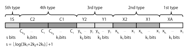
Each type of subrepresentation is allocated to a fixed range of positions, which depends on . Figure 2 illustrates the binary representation of a constructed integer. In Figure 2, each of the types of subrepresentations is distinguished by a kind of shading of gray. For a technical reason, the nd to th types of subrepresentations have copies of them. Such copies are not for the proof for Theorem 20 but for the ones for Theorems 25 and 30. We give each of zones a name as in Figure 2. That is, the names of zones are , , , , , , , and in the descending order from the highest bits.
We describe more details of integers that we construct. Let and be all variables in and , occurring in , respectively. Let be all clauses in . Every constructed integer is represented with bits, where , , and . Each of the , , and zones is of length . Each of the and zones is of length . Each of the and zones is of length . For example, we construct integers for in 16 as illustrated in Table 4. In Table 4, we denote the zone with its decimal representation and the other zones with their binary representations for reflecting the role of each zone.
| Variables | Values | Constructed integers | |||||||
|---|---|---|---|---|---|---|---|---|---|
We describe the detail of the role of each zone of a binary representation that we construct. A constructed integer corresponds to a pair of a Boolean variable and value. Let be a binary representation that we construct.
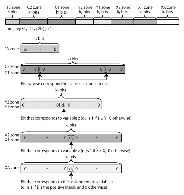
Let us first consider to be one for simulating assigned , where . In the zone, we set the -th bit to and the other bits to s. This means that is assigned and the other variables are assigned . In each of the and zones, we set the -th bit to and the other bits to s. This means that is assigned a Boolean value but the other variables are not assigned. In each of the and zones, we set every bit to . This means that is not for simulating the behavior of a variable in . Moreover, in each of the and zones, for every , we set the -th bit to if the clause includes the literal ; and the other bits to s otherwise. Let be the binary representation of the integer such that is the numbers of s, occurring in the zone. We allocate to the zone of .
Let us next consider to be one for simulating assigned . We set every bit of the zone to . This means that at least is assigned , but does not mean that each of the remaining variables is assigned . The , , , and zones are constructed in the same way as for the case where is assigned . In each of the and zones, for every , we set the -th bit to if the clause includes the literal ; and the other bits to s otherwise. Let be the binary representation of the integer such that is the numbers of s, occurring in the zone. We allocate to the zone of .
Then, let us consider to be one for simulating assigned , where . In each of the , , and zones, we set every bit to . This means that is not for simulating the behavior of a variable in . In each of the and zones, we set the -th bit to and the other bits to s. This means that is assigned a Boolean value but the other variables are not assigned. Note that, in more general, we do not construct the “” part since our concern is on the counting of partial assignments for variables in . In each of the and zones, for every , we set the -th bit to if the clause includes the literal ; and the other bits to s otherwise. Let be the binary representation of the integer such that is the numbers of s, occurring in the zone. We allocate to the zone of . Similarly, we can consider the construction in the case where is one for simulating assigned .
As described above, we simulate an assignment to a variable with an integer. Moreover, for every variable, we construct two integers that correspond to assigned values. Let be the set of integers such that for every variable in , exactly one of the two constructed integers is in . Let be the binary representation of . Then, we can simulate an assignment for with . Every bit in the , , , and zones of is . The zone represent the integer such that , , and are the , , and zones, respectively. The zone corresponds a partial assignment for . Moreover, if every clause contains exactly one true literal, then every bit in the and zones is . That is, for every -assignment , if there is a -assignment such that exactly one true literal exists in every clause, then the assignment is simulated as an integer in the interval , as illustrated in Figure 3.

The above description suggests that we can simulate all assignments for if we correctly select exactly one of the corresponding two integers for every variable in and . However, the reverse direction is more complicated. It is more difficult to verify whether for every variable, exactly one of the corresponding two integers is selected, since, in #NonRep, we can repeatedly select an input integer. Moreover, for a variable , the two integers constructed from the pair of and and the pair of and may be simultaneously selected. Another awkward phenomenon is carrying over in the additions of the integers that we select. Overcoming these difficulties motivates the introduction of the zone. Let be the sum of some integers constructed from and be the binary representation of . If is in and the zone of represents the integer such that , , and are the , , and zones, respectively, then we can consider that no carry occurs in the additions for obtaining .
4.2 Formal discussion for Theorem 20
In this subsection, we prove Theorem 20. As a preparation, we formally define the zones of the binary representation of a positive integer, as informally described in Section 4.1. Let be the binary representation of a positive integer. Then, we call the bit sequence from the st bit to the -th bit the zone of ; the sequence from the -th bit to the -th bit the zone of ; the sequence from the -th bit to the -th bit the zone of ; the sequence from the -th bit to the -th bit the zone of ; the sequence from the -th bit to the -th bit the zone of ; the sequence from the -th bit to the -th bit the zone of ; the sequence from the -th bit to the -th bit the zone of ; and the sequence from the -th bit to the -th bit the zone of .
Proof of Theorem 20. Since [33], we may prove that #NonRep is -complete. We first show that #NonRep is in . Let be an instance of #NonRep. Let be an oracle machine, where is the decision version of the integer knapsack problem ([22], Section 15.7). This problem was proved to be -complete ([22], Section 15.7). First guesses a gap of in the interval . Then, verifies to be in by using oracle . Consequently, #NonRep is in .
In the rest of the proof, we show that #NonRep is -hard under parsimonious reductions by reducing to #NonRep. In particular, we show a polynomial-time computable one-to-one mapping as a parsimonious reduction. We fix to be a -CNF formula over and define an instance of #NonRep, where .
Let and be the integers and , respectively. Let be all clauses of . By the assumption in Section 2.1, is larger than . We suppose that and . We will define as an instance of #NonRep below, where is a set of positive integers and is an interval of positive integers. Every integer in is of the form in Figure 4.
We define as the integer . For every , we define an integer as follows.
Similarly, for every , we define an integer as follows.
We define as . We define positive integers and as follows.
We define as .
Then, we check the time complexity of the reduction. 1 shows the whole of the reduction. In this algorithm, denotes for every where denotes if and ; if and ; if and ; and otherwise. By 1, the reduction can compute in polynomial time.
Claim 21.
can be constructed in polynomial time on the size of .
Proof of Claim 21. It suffices to check , , and all integers in to be computable in time polynomial in , , and . Let be a literal in . The integer consists of at most bits. We can construct each of the , , , , and zones of in time linear in , and . For every clause in , we can check whether is in in constant polynomial. Thus, we construct the and zones of in time polynomial in , , and . After all the zones except the zone are constructed, we can count s in all the zones except the zone in time linear in , , and . Thus, we can calculate the zone in time polynomial in , , and . It follows that is computed in time polynomial in , , and . The integer is calculated in time polynomial in , , and . The set has elements since an integer is defined as an element for every literal in . By the similar method in the above discussion, the integers and can be computed in time polynomial in , , and . Consequently, the claim holds. (Claim 21)
We will check the validity of the above reduction. We show that there is exactly one true literal in every clause in for a given assignment if and only if there is a set such that is in . The “only if” part is straightforward by definition. We show the “if” part here. In the rest of the proof for Theorem 20, we fix to be positive integers in , and to be the sum of , where . For every , we denote the number by .
Claim 22.
For every , exactly one of the following conditions holds.
- 1.
and .
- 2.
and .
To prove Claim 22, it show a more general statement in Claim 24. As preparation, we define some notions and notations for any nonnegative integer . For every , let be a set of integers in . Let be a subset of . We say that is consistent with if can be written as
Note that if is in , then is consistent with . For every , we denote the sum by . We may assume the addition of to do in the left associative manner; i.e., , without loss of generality. Claim 23 is essential although it can be immediately obtained from definitions.
Claim 23.
is consistent with for every if and only if no carry occurs at the , , , , , , and zones in the addition of and for every .
Proof of Claim 23. The “if ” part is trivial by the definitions of integers in . Thus, we prove the “only if” part below. The proof is by induction on . Suppose that is consistent with for every . By induction hypothesis, no carry occurs at the , , , , , , and zones in the addition for every . By definition, every element of is consistent with . Thus, is consistent with . To show that no carry occurs at the , , , , , , and zones in the addition , we separately describe the cases depending on whether a carry occurs at one of the , , , , , and zones in that addition. First, assume that a carry occurs at one of the the , , , , , and zones in that addition. Then,
.
Since is consistent with ,
.
However, in the addition , if a carry occurs at the zone, then at least two carries occur at the and zones since and by their consistencies. It contradicts to the assumption. Hence, no carry occurs at the zone. Next, assume that no carry occurs at the , , , , , and zones in the addition . Then, by the definitions of the , , and zones, no carry occurs at the zone. Consequently, no carry occurs at the , , , , , , and zones in the addition for every . The proof is complete. (Claim 23)
The following claim follows from Claim 23.
Claim 24.
If is consistent with , then the following statements hold.
- 1.
For every with ,
- •
if , then and ,
- •
if , then and ,
- •
otherwise .
- •
- 2.
For every with ,
- •
if , then and ,
- •
otherwise .
- •
Consequently, the theorem holds. (Theorem 25)
5 Complexity of #Bounded NS Gaps
In Section 4, we proved to be parsimonious reducible to #NonRep. In this section, we prove the following theorem by extending the reduction in the proof for Theorem 20 to one from to #Bounded NS Gaps.
Theorem 25.
#Bounded NS Gaps is -complete under parsimonious reductions.
5.1 Ideas of the proof
In this subsection, let be fixed to a -CNF formula over , as in the proof for Theorem 20, where and are disjoint. Similarly, let , and be defined as in the proof for Theorem 20. For extending the reduction in the proof for Theorem 20 to one from to #Bounded NS Gaps, we specify all gaps of in by using another set that contains as a subset. In more detail, we construct the mapping so that .
5.1.1 Observation
First, we describe how to specify every integer in as a gap of another numerical semigroup, which is larger than a bound. Let us first consider a toy example of #NonRep instead of an input constructed from a -CNF formula. Let be the set . We observe an example illustrated in Figure 5.

In Figure 5, all the circles on the three lines mean integers in . On every line, the grayed circles mean positive integers given as inputs. The black circles mean positive integers, each of which can be written as a nonnegative integer combination of the input positive integers but is not one of the input positive integers themselves. The white circles mean other integers in ; i.e., integers that cannot be written as nonnegative integer combinations of the corresponding input integers. The circles on the st line illustrate a part of . That is, we can observe an instance of #Bounded NS Gaps on the st line.
Let us next specify two gaps and of in with another numerical semigroup and only the lower bound but without the upper bound . For this purpose, we may find a numerical semigroup such that . A simple but naive approach to specify is by using as its generators. The nd line of Figure 5 illustrates . By definition, contains successive integers from to . The number of these successive integers is not smaller than the smallest element of . This fact guarantees that does not include any integer greater than . Unfortunately, the size of is of exponential order in the size of since we assume the size of an integer to be its bit length. This defect is caused by the cardinality of .
For making the number of generators of smaller, it suffices to specify every integer between and as a nonnegative integer combination of a smaller set of positive integers. More generally, it is not so difficult since we can specify every integer in an interval of positive integers as a nonnegative integer combination of positive integers for some . However, we have to be careful to preserve all gaps of between and . If is the set , then satisfies the above conditions. As illustrated on the rd line in Figure 5, all integers in greater than are included by , which are and , and does not contain any gap of in , which are and .
5.1.2 An example of our reduction
Next, we illustrate the reduction that we will formulate in Section 5.2 by using an example. Let be a -CNF formula , where and . Table 5 shows clauses, each of which contains exactly one true clause for every assignment for .
| — | ||||
| — | ||||
| — | — | |||
| — | — | |||
| Arguments of | Constructed integers | ||||||||
|---|---|---|---|---|---|---|---|---|---|
| Variables | Values | ||||||||
| Endpoints | Constructed integers | |||||||
|---|---|---|---|---|---|---|---|---|
Tables 6 and 7 show integers constructed from by using the reduction in the proof for Theorem 20. Tables 8 and 9 show integers that we will construct. Moreover, we define as the integer . This is defined from by the same method for in the reduction in the proof for Theorem 20.
The numerical semigroup generated by the integers in Tables 8 or 9 satisfies the conditions that we described in 5.1.1. For every integer , if is greater than , then can be represented as a nonnegative integer combination of and integers in Tables 8 or 9; and otherwise, cannot be represented by the same way. Intuitively speaking, every integer in Tables 8 or 9 is a kind of dummy. In Tables 8 and 9, every row is tagged with a variable or a clause in the st column, although any integer does not have a role for simulating a -CNF formula. If we select integers, one each for every variable and clause in Tables 8 and 9, then we can represent an integer greater than as their sum, and vice versa.
We describe the details of integers in Tables 8 or 9. Let be the binary representation of an integer between the st and th rows in Table 8. is tagged with a variable in . Let be if is tagged with ; and otherwise. In each of the , , and zones of , occurs at most once. Conversely, in at least one of the , , and zones, occurs. In each of the and zones, if occurs, then its position is the -th bit of the zone. In the zone, if occurs, then its position is the -th bit of the zone, where the modulus is from the cardinality of . As described above, every integer in Tables 8 or 9 is for representing all integers larger than but not for simulating a -CNF formula. Thus, for avoiding improperly simulating a -CNF formula, the position of the bit of is shifted in the zone.
Similarly, in Tables 8 or 9, every integer between the rd and th rows is tagged with a variable in . Moreover, every integer between the th and th rows is tagged with a clause in .
For every , let be a binary representation in Table 8, which is tagged with . In , the integer represented by its zone is equal to , where is the maximum number of occurrences of s in its remaining zones among all integers tagged with in Table 8. On the other hand, in Table 9, the integer represented in its zone is equal to , where is the maximum number of occurrences of s in its remaining zones. The difference of the zones in integers in Tables 8 and 9 is for representing every integer greater than as a sum of and integers that we select one each for every variable and clause in .
| Variables | Values | Constructed integers | |||||||
|---|---|---|---|---|---|---|---|---|---|
| or clauses | |||||||||
| Variables | Values | Constructed integers | |||||||
|---|---|---|---|---|---|---|---|---|---|
| or clauses | |||||||||
5.2 Formal discussion for Theorem 25
Proof of Theorem 25. First, we prove that #Bounded NS Gaps is in , i.e., . By Theorem 20, it suffices to show that #Bounded NS Gaps is a special case of #NonRep as follows. Let be an instance of #Bounded NS Gaps. Let be the maxmum element of . By definition, all integers in are coprime. Thus, there is the maximum element in . By an upper bound for [38], is equal to . Thus, #Bounded NS Gaps is an special case of #NonRep. Consequently, #Bounded NS Gaps is in .
Next, we prove that #Bounded NS Gaps is -hard under parsimonious reductions. For this purpose, we reduce to #Bounded NS Gaps. Let , , , , , and be given as in the proof for Theorem 20. is a -CNF formula over . , , and are , , and , respectively. Let and be defined as in the proof for Theorem 20. is a polynomial-time computable function from -CNF-formulae to positive integers. is a set of positive integers. is an interval of positive integers. and is a positive integer. By the proof for Theorem 20, we can construct and in polynomial time.
For , we will define a function such that
is equal to , where is the set defined in Section 2.4. Then, we will define dummy integers described in Section 5.1. For every , , we define an integer as
Figure 6 illustrates the binary representation of .

Similarly, for every , , we define an integer as
Figure 7 illustrates the binary representation of .

For every clause with and , we define an integer as
Figure 8 illustrates the binary representation of .

For every , we denote the set by . For every , we denote the set by .
For every and , we define as ; i.e., is the integer obtained from by incrementing its zone. We denote the set by . Moreover, we denote the set
by . We define as the set
By 2, the reduction can compute in polynomial time.
Then, we show the validity of the reduction. In the rest of the proof for Theorem 25, let be integers in and let be the sum of . For every , let be . That is, and . For any nonnegative integer , we say that is consistent with if satisfies the same condition as in the proof for Theorem 20. Note that this notion is well-defined for any nonnegative integer. Moreover, by definition, if is in , then is consistent with . We can prove the following claim by the similar discussion as in the proof for Claim 23.
Claim 26.
is consistent with for every if and only if no carry occurs at the , , , , , , and zones in the addition for every .
Claim 27.
If and there is no such that , then .
Proof of Claim 27. Let be in . Let be a subset of and be a subset of such that . By assumption, if , then and , which is a contradiction. Thus, is nonempty. Assume that and is in . Then, by the definitions of integers in or , at least one carry occurs in one of the zones. This contradicts to Claim 26. (Claim 27)
Claim 28.
If , then we can find a set such that .
Proof of Claim 28. By the definitions of integers in , we can represent every integer in as a nonnegative integer combination of . Thus, the claim holds. (Claim 28)
Claim 29.
All integers in are coprime.
6 Complexity of #NS Gaps
In this section, we prove Theorem 30 by extending the reduction in the proof for Theorem 25 to a reduction from to #NS Gaps. Theorem 30 is a main theorem in this paper.
Theorem 30.
#NS Gaps is -complete under relaxed subtractive reductions.
6.1 Closure property of under relaxed subtractive reductions
In Section 2.3, we introduced a new type of polynomial-time reduction that we call a relaxed subtractive reduction. In this subsection, we prove that is closed under relaxed subtractive reductions. The proof takes the same approach as the proofs for the closure property of under subtractive reductions in [10] and complementive reductions in [4].
Theorem 31.
For every , the class is closed under relaxed subtractive reductions.
Proof of Theorem 31. Let and be counting problems. Suppose that . Let a pair of polynomial-time computable functions be a relaxed subtractive reduction from to and be a decision problem such that , which satisfy the following conditions. For every ,
- 1.
- 2.
- 3.
- 4.
.
These conditions are from the definition of a strong relaxed subtractive reduction. For proving the theorem, it suffices to show that
- (S1)
there is a decision problem such that ,
- (S2)
for every .
By the equality [33], the statement (S1) implies that . The statements (S1) and (S2) imply that .
Let be a deterministic oracle machine that recognizes , where is an oracle in . By the equality , is in . Let consist of all pairs such that , , and , where is a new symbol. We show that is a witness of by using a deterministic oracle machine . simulates as a subroutine with overhead bounded by a polynomial in the size of .
Let be . We can extract from in polynomial time. Moreover, we can check whether is obtained from in polynomial time, since is a polynomial-time computable function. We can do the same process for in . After doing these processes, we extract from . We can do this process in polynomial time. Then, we check that is in . By using as a subroutine, we can check that is in in polynomial time. Similarly, we can execute the following steps in polynomial time. We extract from and check that are not in . Finally, we check to be not in . We can execute this step in polynomial time since we assume to be in . Thus, is in . By definition, is equal to .
By assumption, is . Thus, is equal to . This implies that . Consequently, is in . The proof is complete.
6.2 Ideas and examples of the reduction
In this subsection, we describe main ideas of our reduction from to #NS Gaps. In Section 5, we proved that is parsimonious reducible to #Bounded NS Gaps. This implies that is also relaxed subtractive reducible to #Bounded NS Gaps. By extending the reduction in the proof for Theorem 25, we will construct a strong relaxed subtractive reduction from to #NS Gaps.
Let , and be as in the proof for Theorem 25. Our goal is obtaining a function and a problem , which satisfy the following conditions.
- (C1)
Every integer in is in .
- (C2)
coincides .
As a result, we want to construct a (strong) relaxed subtractive reduction such that
Let us informally describe the relaxed subtractive reduction by using examples. For observing essential properties of numerical semigroups for our reduction, we first consider a simple example such that a pair of a set of positive integers and an interval are given but may not be constructed from a -CNF formula. Let be given, where . We simulate every integer in as an integer in as in Figure 9, where and . coincides with . In Figure 9, every circle means an integer. The st two lines correspond to the numerical semigroups generated by and , respectively. On these two lines, every black circle means a nongap of or . Every gray circle means an element of or . Every white circle means a gap of or . The rd line corresponds to . On this line, every white circle means an element of .

We can specify all integers of by its two partitions. This partitions are defined by depending on whether an integer is in . In Figure 9, coincides with . coincides with .
Let us next consider an instance of #NS Gaps, which is defined for an instance of . Let be the -CNF formula as in 5.1.2. Let be a set consisting of and all integers in Tables 6, 8 or 10. Let be a set consisting of and all integers in Tables 6, 8, 9, or 10. Then, we specify all integers in as follows. Since is a subset of , contains as a subset; i.e., any integer that cannot be represented as a nonnegative integer combination of cannot be done as of . Thus, the task that is left is a specification of . Let be . Moreover, we can observe that does not include any integer of by checking each bit in the binary representation of each integer in and the integer .
| Variables | Values | Constructed integers | |||||||
|---|---|---|---|---|---|---|---|---|---|
| or clauses | |||||||||
6.3 Formal discussion for Theorem 30
Proof of Theorem 30. By definition #NS Gaps is a special case of #Bounded NS Gaps. Thus, by Theorem 25, #NS Gaps is in . All that is left is to prove #NS Gaps to be -hard under relaxed subtractive reductions.

Let be given as in the proof for Theorem 25. Let , , , , and be defined as in the proof for Theorem 25. We will define a function and find a decision problem such that
- (C1)
,
- (C2)
,
- (C3)
,
- (C4)
There is a such that for every if and only if there is an integer in .
Figure 10 illustrates relationships of , , and . Let be the set . coincides with . We define as
We can check that can be constructed in polynomial time by the same discussion as for in the proof of Theorem 25.
Next, we define as a decision problem. We define the polynomially balanced binary relation as follows. A pair is in if and only if is a -CNF formula and is the sum of all positive integers in a set . satisfies the following conditions.
- •
Exactly one of and is in .
- •
For every , at most one element in is in .
- •
For every , at most one element in is in .
Then, an instance of is a -CNF over , the question of is whether there is an integer such that . By definition, is in . Moreover, is ; i.e., , which is computable in time polynomial in , and . Thus, the counting problem is in .
In the rest of the proof for Theorem 30, we will show the validity of the above construction. Let be integers in and let be the sum of . For every , let be . For any nonnegative integer , we say that is consistent with if satisfies the same condition as in the proof for Theorem 25. We can prove the following claim by the similar discussion in the proof for Theorems Theorem 20 and Theorem 25.
Claim 32.
is consistent with for every if and only if no carry occurs at the , , , , , , and parts in the addition for every .
Claim 33.
If , then we can find a set such that .
Claim 34.
If and there is no such that , then .
Claim 35.
Let be less than . if and only if there is an such that and there is no such that
We can observe the validities of the statements of Claims 33, 34, and 35 by using examples of Figure 9. Let , , and be as in Section 6.2. and correspond to , , and , respectively. Claim 33 corresponds to the fact that every integer greater than or equal to the lower endpoint can be represented as a nonnegative integer combination of . Claim 34 corresponds to the fact that cannot be represented as a nonnegative integer combination of . Claim 35 corresponds to the fact that and are in and can be represented as nonnegative integer combinations of but cannot of . The following claim follows from Claim 29.
Claim 36.
All integers in are coprime.
7 Future work
In this paper, we proved the -completeness of #NS Gaps under relaxed subtractive reductions as a main result. A relaxed subtractive reduction is new type of polynomial-time reduction. Moreover, we proved the -completenesses of #NonRep and #Bounded NS Gaps, which are variants of #NS Gaps, under parsimonious reductions. This section describes future work.
7.1 -hardness of #NS Gaps under parsimonious reductions
We showed the -completeness of #NS Gaps under relaxed subtractive reductions. It is natural to ask whether #NS Gaps is -complete under parsimonious reductions. Unfortunately, it appears to be quite difficult to answer this question.
In this paper, we mainly use combinatorial and logical approaches for constructing reductions, but use little result in number theory. Thus, it may be possible to prove #NS Gaps to be -complete under parsimonious reductions by using some tools developed in number theory. Cook [7] said that the primality testing problem requires a deep insight on number theory. Indeed, over thirty years later, [1] found a polynomial-time algorithm by an approach from number theory.
7.2 Proof methods for the -hardness of #Bounded NS Gaps
To prove the hardness of #Bounded NS Gaps, we reduced to #Bounded NS Gaps. However, a reduction from #NonRep to #Bounded NS Gaps is another natural reduction. Since the latter reduction is a self-reduction, it appears to be more natural than our reduction. Nevertheless, we could not adopt this approach by the following obstacle.
A parsimonious reduction from #NonRep to #Bounded NS Gaps requires a deep insight into number theoretical aspects of numerical semigroups. Given an instance of #NonRep, no polynomial-time algorithm is known for finding an instance of #Bounded NS Gaps such that
- (C1)
and
- (C2)
the size of is of polynomial order in the size of .
To the best of the author’s knowledge, little relationship is known for an instance of #Bounded NS Gaps and an instance of #NonRep. Our reduction in Section 5 makes use of properties originated from an instance of .
7.3 Completeness for under more general reductions
We introduced relaxed subtractive reductions as a generalization of subtractive reductions. Moreover, relaxed subtractive reductions are also special case of polynomial-time bounded truth-table reductions [19]. As a property of this type of reduction, relaxed subtractive reductions have nonadaptivity; i.e., all oracle queries must be decided before starting the other processes. Moreover, in every relaxed subtractive reduction, its normal processes are also independent of its two oracle queries. We can consider that a -complete problem exists under relaxed subtractive reductions due to this property. However, we do not know whether there is a more general type of nonadaptive reduction under which is closed. This is an interesting subject since is not closed under polynomial-time Turing reductions [35].
References
- [1] Manindra Agrawal, Neeraj Kayal, and Nitin Saxena. PRIMES is in P. Annals of Mathematics, 160(2):781–793, 2004.
- [2] Sanjeev Arora and Boaz Barak. Computational Complexity: a Modern Approach. Cambridge University Press, New York, NY, 2009.
- [3] Alexander Barvinok and Kevin Woods. Short rational generating functions for lattice point problems. Journal of the American Mathematical Society, 16(4):957–979, 2003.
- [4] Michael Bauland, Elmar Böhler, Nadia Creignou, Steffen Reith, Henning Schnoor, and Heribert Vollmer. The complexity of problems for quantified constraints. Theory of Computing Systems, 47(2):454–490, 2010.
- [5] Dale Beihoffer, Jemimah Hendry, Albert Nijenhuis, and Stan Wagon. Faster algorithms for Frobenius numbers. The Electronic Journal of Combinatorics, 12(#R27), 2005.
- [6] Ashok K. Chandra, Dexter C. Kozen, and Larry J. Stockmeyer. Alternation. J. ACM, 28:114–133, January 1981.
- [7] Stephen A. Cook. The complexity of theorem-proving procedures. In Proceedings of the third annual ACM symposium on Theory of computing, STOC ’71, pages 151–158, New York, NY, USA, 1971. ACM.
- [8] Nadia Creignou and Miki Hermann. Complexity of generalized satisfiability counting problems. Information and Computation, 125(1):1–12, 1996.
- [9] Ding-Zhu Du and Ker-I Ko. Theory of Computational Complexity. John Wiley & Sons, 2000.
- [10] Arnaud Durand, Miki Hermann, and Phokion G. Kolaitis. Subtractive reductions and complete problems for counting complexity classes. Theoretical Computer Science, 340(3):496–513, 2005.
- [11] David Einstein, Daniel Lichtblau, Adam Strzebonski, and Stan Wagon. Frobenius numbers by lattice point enumeration. Integers, 7(1):A15, 2007.
- [12] Michael R Garey and David S Johnson. Computers and Intractability: a Guide to NP-Completeness. WH Freeman, New York, NY, 1979.
- [13] Ronald L. Graham, Donald E. Knuth, and Oren Patashnik. Concrete Mathematics: a Foundation for Computer Science. Addison-Wesley Longman Publishing Co., Inc., Boston, MA, 2nd edition, 1994.
- [14] Lane A. Hemaspaandra and Heribert Vollmer. The satanic notations: Counting classes beyond and other definitional adventures. SIGACT News, 26(1):2–13, March 1995.
- [15] Miki Hermann and Reinhard Pichler. Complexity of counting the optimal solutions. Theoretical Computer Science, 410(38-40):3814–3825, 2009.
- [16] Miki Hermann and Reinhard Pichler. Counting complexity of propositional abduction. Journal of Computer and System Sciences, 76(7):634–649, 2010.
- [17] Ravi Kannan. Lattice translates of a polytope and the Frobenius problem. Combinatorica, 12(2):161–177, 1992.
- [18] Mark W. Krentel. Generalizations of opt p to the polynomial hierarchy. Theoretical Computer Science, 97(2):183–198, 1992.
- [19] R.E. Ladner, N.A. Lynch, and A.L. Selman. A comparison of polynomial time reducibilities. Theoretical Computer Science, 1(2):103–123, 1975.
- [20] Shunichi Matsubara. The computational complexity of the Frobenius problem. CoRR, abs/1602.05657, 2016.
- [21] A. R. Meyer and L. J. Stockmeyer. The equivalence problem for regular expressions with squaring requires exponential space. In Proceedings of the 13th Annual Symposium on Switching and Automata Theory, SWAT ’72, pages 125–129, Washington, DC, USA, 1972. IEEE Computer Society.
- [22] Christos H. Papadimitriou and Kenneth Steiglitz. Combinatorial Optimization: Algorithms and Complexity. Prentice-Hall, Inc., Upper Saddle River, NJ, 1982.
- [23] Cristos H. Papadimitriou. Computational Complexity. Addison-Wesley Publishing, 1994.
- [24] Jorge L Ramírez Alfonsín. Complexity of the Frobenius problem. Combinatorica, 16(1):143–147, 1996.
- [25] Jorge L Ramírez Alfonsín. The Diophantine Frobenius Problem. Oxford University Press, Oxford, 2005.
- [26] José C Rosales and Pedro A García-Sánchez. Numerical Semigroups, volume 20. Springer Science & Business Media, 2009.
- [27] Bjarke Hammersholt Roune. Solving thousand-digit Frobenius problems using Gröbner bases. Journal of Symbolic Computation, 43(1):1–7, 2008.
- [28] Thomas J. Schaefer. The complexity of satisfiability problems. In Proceedings of the Tenth Annual ACM Symposium on Theory of Computing, STOC ’78, pages 216–226, New York, NY, USA, 1978. ACM.
- [29] Marcus Schäfer and Christopher Umans. Completeness in the polynomial-time hierarchy: Part I: a compendium. SIGACT News, 33(4):22–36, December 2002.
- [30] Marcus Schäfer and Christopher Umans. Guest column: Completeness in the polynomial-time hierarchy: Part II. SIGACT News, 33(3):32–49, 2002.
- [31] Larry J. Stockmeyer. The polynomial-time hierarchy. Theoretical Computer Science, 3(1):1–22, 1976.
- [32] J. J. Sylvester. On subvariants, i.e. semi-invariants to binary quantics of an unlimited order. American Journal of Mathematics, 5(1):79–136, 1882.
- [33] Seinosuke Toda. Computational Complexity of Counting Complexity Classes. Ph.D. dissertation, Tokyo Institute of Technology, 1991.
- [34] Seinosuke Toda. PP is as hard as the polynomial-time hierarchy. SIAM Journal on Computing, 20(5):865–877, October 1991.
- [35] Seinosuke Toda and Osamu Watanabe. Polynomial-time 1-Turing reductions from to . Theoretical Computer Science, 100(1):205–221, 1992.
- [36] Leslie G. Valiant. The complexity of computing the permanent. Theoretical Computer Science, 8(2):189–201, 1979.
- [37] Leslie G. Valiant. The complexity of enumeration and reliability problems. SIAM Journal on Computing, 8(3):410–412, August 1979.
- [38] Herbert S. Wilf. A circle-of-lights algorithm for the “money-changing problem”. The American Mathematical Monthly, 85(7):562–565, 1978.
- [39] Celia Wrathall. Complete sets and the polynomial-time hierarchy. Theoretical Computer Science, 3(1):23–33, 1976.