跳到论文正文
W Papers独立论文阅读器 arXiv:1609.06347 论文正文 计算阅读时间 · 0%
引用这篇论文根据当前论文元数据生成,正式投稿前建议核对。


License: arXiv.org perpetual non-exclusive license
arXiv:1609.06347v2 [nlin.CD] 10 Aug 2017

Stabilizing Embedology: Geometry-Preserving
Delay-Coordinate Maps

Armin Eftekhari    Han Lun Yap    Michael B. Wakin    Christopher J. Rozell Note: The first two authors contributed equally, as did the last two authors. AE is with the Alan Turing Institute. HLY is with DSO National Laboratories of Singapore. MBW is with the Department of Electrical Engineering and Computer Science at the Colorado School of Mines. CJR is with the School of Electrical and Computer Engineering at the Georgia Institute of Technology. Email: crozell@gatech.edu. This work was partially supported by NSF grants CCF-0830320, CCF-0830456, CCF-1409258, and CCF-1409422; NSF CAREER grant CCF-1350954; and James S. McDonnell Foundation grant number 220020399.
Abstract

Delay-coordinate mapping is an effective and widely used technique for reconstructing and analyzing the dynamics of a nonlinear system based on time-series outputs. The efficacy of delay-coordinate mapping has long been supported by Takens’ embedding theorem, which guarantees that delay-coordinate maps use the time-series output to provide a reconstruction of the hidden state space that is a one-to-one embedding of the system’s attractor. While this topological guarantee ensures that distinct points in the reconstruction correspond to distinct points in the original state space, it does not characterize the quality of this embedding or illuminate how the specific parameters affect the reconstruction. In this paper, we extend Takens’ result by establishing conditions under which delay-coordinate mapping is guaranteed to provide a stable embedding of a system’s attractor. Beyond only preserving the attractor topology, a stable embedding preserves the attractor geometry by ensuring that distances between points in the state space are approximately preserved. In particular, we find that delay-coordinate mapping stably embeds an attractor of a dynamical system if the stable rank of the system is large enough to be proportional to the dimension of the attractor. The stable rank reflects the relation between the sampling interval and the number of delays in delay-coordinate mapping. Our theoretical findings give guidance to choosing system parameters, echoing the trade-off between irrelevancy and redundancy that has been heuristically investigated in the literature. Our initial result is stated for attractors that are smooth submanifolds of Euclidean space, with extensions provided for the case of strange attractors.

Keywords— Nonlinear time-series analysis, Delay-coordinate mapping, Takens’ embedding theorem, Method of delays, State space, Attractor, Smooth manifold, Stable rank

1 Introduction

1.1 Motivation and Contribution

Modern science is ingrained with the premise that repeated observations of a dynamic phenomenon can help us understand its underlying mechanisms and predict its future behavior. While this idea dates back to ancient times with the observation of sunspots [68], today we model the behavior of a wide variety of measured phenomena from the life, physical, and social sciences [10, 7, 39, 58, 50, 28, 48, 69, 64, 32] as observations arising from complex dynamical systems. Understanding and predicting a time series is often approached by postulating a structured model for a hidden dynamical system that drives the data generation. Linear statistical models were used in early work [72] and are now reflected in standard tools such as the autoregressive-moving-average model and the Kalman filter (e.g., [4]). More recently, the field of nonlinear time-series analysis models time-series data as observations of the state of a (possibly high-dimensional) deterministic nonlinear dynamical system [32]. While the underlying dynamical system may exhibit chaotic behavior, it is often postulated as being governed by an attractor that is a low-dimensional geometric subset of the state space.

Due to the low-dimensional behavior in the underlying state space, it is reasonable to postulate that temporal dependencies in time-series observations can provide some insight into the structure of the hidden dynamical system. This leads to a fundamental question: How much information about a hidden dynamical system is available in time-series measurements of the system state? The seminal Takens’ embedding theorem [59, 51] asserts that (under very general conditions) it is possible to use the time-series data to reconstruct a state-space that is a topologically-equivalent image of the attractor through a simple procedure known as the delay-coordinate map. Indeed, many algorithms for tasks such as time-series prediction and dimensionality estimation take inspiration and justification from this fundamental guarantee [17, 26, 33, 65, 36, 67, 3, 6, 29]. While the topological guarantee of Takens’ theorem provides that the delay-coordinate map is one-to-one (i.e., distinct points in the reconstruction correspond to distinct points in the original state space), it does not speak to the overall quality of the reconstruction or how this quality is affected by specific details such as the algorithm parameters, the measurement function, or the system characteristics.

Many fields of data science also rely on capturing low-dimensional structure from high-dimensional data, and recent advances have shown the value of guaranteeing geometric stability of an embedding as a measure of quality for subsequent inference. In such a stable embedding, the embedding approximately preserves the distance between any two points in the data set of interest, which has proven to be valuable for robustness to imperfections in many forms (i.e., noise, numerical imprecision, etc.). In computer science, the Johnson-Lindenstrauss lemma constructs stable embeddings for finite point clouds using random linear projections [19]. In compressive sensing [22, 13], the Restricted Isometry Property (RIP) condition captures the notion of a stable embedding for sparse signal families, ensuring that signal reconstruction from random linear measurements is robust to noise and stable with respect to model nonidealities [14]. For dimensionality reduction with signal families belonging to low-dimensional manifolds and more general sets, various types of stable embeddings have been constructed using adaptive nonlinear techniques such as ISOMAP [61], adaptive linear techniques [11, 30], and nonadaptive linear techniques that again employ randomness [46, 23, 18, 71].

The main contribution of this paper is to extend the notion of Takens’ embedding theorem to stable embeddings, providing insight into the conditions for when time-series data can (and cannot) be used to reconstruct a geometry-preserving image of the attractor. In addition to providing the formal foundations to justify the numerical algorithms based on delay-coordinate mapping, these results also give guidance to practitioners about how algorithm and observation design choices affect the overall quality of the representation. In particular, examination of our main theoretical findings gives guidance to choosing these system parameters, echoing the trade-off between irrelevancy and redundancy that has been heuristically investigated in the literature. For clarity and to gain as much insight as possible, our main result is first described for attractors that are smooth submanifolds of the Euclidean space (similar to Takens’ original result) and then extended to the case of strange attractors. The remainder of the Introduction will provide a simplified version of the main result to give the flavor of the contribution from this paper, with the full technical results given in Sections 3.3 (smooth manifolds) and 3.5 (strange attractors). To streamline readability as much as possible, the proofs and additional technical details are contained in appendices for the interested reader.

1.2 Delay-Coordinate Maps and Takens’ Embedding Theorem

We consider x⁡(⋅)x(\cdot) as the trajectory of a dynamical system in the state space ℝN\mathbb{R}^{N} such that x⁡(t)∈ℝNx(t)\in\mathbb{R}^{N} for t∈[0,∞)t\in[0,\infty). While the system has continuous underlying dynamics, we observe this system at a regular sampling interval T>0T>0. Given this sampling interval, one may define the discrete dynamics in terms of the flow ϕT:ℝN→ℝN\phi_{T}:\mathbb{R}^{N}\rightarrow\mathbb{R}^{N} such that x⁡(t+T)=ϕT​(x⁡(t))x(t+T)=\phi_{T}(x(t)). In words, ϕT​(⋅)\phi_{T}(\cdot) moves the system state into the future by TT. We assume that during the times of interest the state trajectory is contained within a low-dimensional attractor [32] 𝔸\mathbb{A} such that x⁡(t)∈𝔸⊂ℝNx(t)\in\mathbb{A}\subset\mathbb{R}^{N} for t≥0t\geq 0. The attractor 𝔸\mathbb{A} is assumed to be a bounded, boundary-less, and smooth submanifold of ℝN\mathbb{R}^{N} with dim⁡(𝔸)<N\operatorname{dim}(\mathbb{A)}<N. The flow operator restricted to this attractor is a diffeomorphism on 𝔸\mathbb{A} so that there exists a smooth inverse ϕT−1​(x⁡(t))=x⁡(t−T)\phi_{T}^{-1}(x(t))=x(t-T).

In applications of interest we often cannot directly observe this system state but rather receive indirect measurements via a scalar measurement function h:𝔸→ℝh:\mathbb{A}\rightarrow\mathbb{R}. This function generates a single scalar measurement at a regular sampling interval T>0T>0, producing the resulting discrete time series {si}i∈ℕ={h⁡(x⁡(i⋅T))}i\{s_{i}\}_{i\in\mathbb{N}}=\{h(x(i\cdot T))\}_{i}, where each si∈ℝs_{i}\in\mathbb{R}. The goal is to “reconstruct” the hidden state trajectory x⁡(⋅)x(\cdot) given only {si}i\{s_{i}\}_{i}. To approach this task, consider the delay-coordinate map Fh,T,M:𝔸→ℝMF_{h,T,M}:\mathbb{A}\rightarrow\mathbb{R}^{M}, defined for an integer number of delays MM through the relation

Fh,T,M​(x⁡(i⋅T))=[sisi−1⋮si−M+1]=[h⁡(x⁡(i⋅T))h⁡(x⁡((i−1)⋅T))⋮h⁡(x⁡((i−M+1)⋅T))]=[h⁡(x⁡(i⋅T))h⁡(ϕT−1​(x⁡(i⋅T)))⋮h⁡(ϕT−M+1​(x⁡(i⋅T)))].F_{h,T,M}\left(x(i\cdot T)\right)=\left[\begin{array}[]{c}s_{i}\\ s_{i-1}\\ \vdots\\ s_{i-M+1}\end{array}\right]=\left[\begin{array}[]{c}h(x(i\cdot T))\\ h\left(x((i-1)\cdot T)\right)\\ \vdots\\ h\left(x((i-M+1)\cdot T)\right)\end{array}\right]=\left[\begin{array}[]{c}h(x(i\cdot T))\\ h\left(\phi_{T}^{-1}(x(i\cdot T))\right)\\ \vdots\\ h\left(\phi_{T}^{-M+1}(x(i\cdot T))\right)\end{array}\right]. (1)

Note that the delay-coordinate map is simply formed at a given time by stacking the last MM observed time-series values into a vector. Commonly, ℝM\mathbb{R}^{M} is referred to as the reconstruction space.

Takens’ embedding theorem [59, 51] asserts that it is indeed possible to reconstruct the state space from the time-series data. With this setup, Takens’ result roughly states that if M>2⋅dim⁡(𝔸)M>2\cdot\operatorname{dim}(\mathbb{A)}, then the delay-coordinate map Fh,T,M​(⋅)F_{h,T,M}(\cdot) resulting from almost every smooth measurement function h⁡(⋅)h(\cdot) embeds the attractor 𝔸\mathbb{A} into the reconstruction space ℝM\mathbb{R}^{M} (i.e., the delay-coordinate map forms a diffeomorphism for 𝔸\mathbb{A}). In other words, the topology of the attractor 𝔸\mathbb{A} is preserved in the reconstruction space ℝM\mathbb{R}^{M} under the delay-coordinate map, and therefore the trajectory in the reconstruction space Fh,T,M​(x​(⋅))F_{h,T,M}(x(\cdot)) is (in principle) equivalent to the trajectory in the state space x⁡(⋅)x(\cdot). Figure 1 illustrates the concept of a delay-coordinate map in the case of the widely-known Lorenz attractor. Despite this embedding guarantee ensuring that no two points from the attractor map onto each other in the reconstruction, the mapping could be unstable in the sense that close points may map to points that are far away (and vice versa). While the simplified main result of this paper is presented for the case of attractors that are smooth submanifolds, the extensions presented in Section 3.5 include strange attractors such as the Lorenz attractor.

(a) State space
(b) Time series
(c) Reconstruction space
Figure 1: (a) The state space trajectory of the Lorenz attractor in ℝ3\mathbb{R}^{3}, demonstrating the characteristic butterfly pattern. (b) The time series obtained by a measurement function that only keeps the x1x_{1}-coordinate of the trajectory. (c) The delay-coordinate map points with M=2M=2, recreating the butterfly pattern using only the time series.

1.3 Simplified Main Result

To quantify the quality of the embedding in the reconstruction space, we seek the stronger guarantee that the delay-coordinate map Fh,T,M​(⋅)F_{h,T,M}(\cdot) is a stable embedding of the attractor 𝔸\mathbb{A}. By stable embedding, we mean that Fh,T,M​(⋅)F_{h,T,M}(\cdot) must act as a near-isometry on 𝔸\mathbb{A}, in the sense that

ϵl≤‖Fh,T,M​(x)−Fh,T,M​(y)‖22M⋅‖x−y‖22≤ϵu,∀x,y∈𝔸,x≠y\epsilon_{l}\leq\frac{\left\|F_{h,T,M}(x)-F_{h,T,M}(y)\right\|_{2}^{2}}{M\cdot\|x-y\|^{2}_{2}}\leq\epsilon_{u},\qquad\forall x,y\in\mathbb{A},\penalty\ x\neq y (2)

for some isometry constants 0<ϵl≤ϵu<∞0<\epsilon_{l}\leq\epsilon_{u}<\infty. Said another way, if ϵl≈ϵu\epsilon_{l}\approx\epsilon_{u}, the stable embedding condition of (2) guarantees that the delay-coordinate map preserves the geometry of the attractor (rather than merely its topology) by ensuring that pairwise distances between points on the attractor are approximately preserved in the reconstruction space. Since x⁡(⋅)⊂𝔸x(\cdot)\subset\mathbb{A}, the same would hold for the trajectory and its image, thereby guaranteeing the quality of the trajectory embedding in the reconstruction space ℝM\mathbb{R}^{M}.

The main result of this paper is to determine the conditions on the attractor 𝔸\mathbb{A}, measurement function h⁡(⋅)h(\cdot), number of delays MM, and sampling interval TT such that Fh,T,M​(⋅)F_{h,T,M}(\cdot) is a stable embedding of 𝔸\mathbb{A}. This is a more ambitious objective than Takens’ embedding theorem (leading naturally to more restrictive conditions), but with the benefit of quantifying the quality of the embedding and relating that quality to the problem-specific parameters. Roughly speaking, our main result shows that Fh,T,M​(⋅)F_{h,T,M}(\cdot) stably embeds 𝔸\mathbb{A} (in the sense of (2)) for most measurement functions hh, provided that the following condition is satisfied:

RH,T,M⁡(𝔸)≳dim⁡(𝔸)⋅log⁡(vol⁡(𝔸)1dim⁡(𝔸)rch⁡(𝔸)).\operatorname{R}_{H,T,M}(\mathbb{A})\gtrsim\operatorname{dim}(\mathbb{A})\cdot\log\left(\frac{\operatorname{vol}(\mathbb{A})^{\frac{1}{\operatorname{dim}(\mathbb{A})}}}{\operatorname{rch}(\mathbb{A})}\right). (3)

Here, dim⁡(𝔸)\operatorname{dim}(\mathbb{A}) and vol⁡(𝔸)\operatorname{vol}(\mathbb{A}) are the dimension and volume of the attractor 𝔸⊂ℝN\mathbb{A}\subset\mathbb{R}^{N}, and rch⁡(𝔸)\operatorname{rch}(\mathbb{A}) is an attribute of 𝔸\mathbb{A} that captures its geometric regularity. To quantify the notion of “most” measurement functions, our result is probabilistic and holds with high probability over measurement functions drawn from a rich probability model HH. The stable rank RH,T,M⁡(𝔸)\operatorname{R}_{H,T,M}(\mathbb{A}) of 𝔸\mathbb{A} quantifies the ability of the random measurement functions to observe the system attractor. Both reach and stable rank are well-studied concepts, and will be discussed (along with the detailed probability model HH) in full technical detail later.

Typically, if a dynamical system is fairly “predictable”, then RH,T,M⁡(𝔸)\operatorname{R}_{H,T,M}(\mathbb{A}) grows proportionally with MM as the number of delays grows. In this case, the delay-coordinate map stably embeds 𝔸\mathbb{A} when the number of delays scales linearly with the dimension of the attractor as in Takens’ original theorem. On the other hand, if the dynamical system is highly unpredictable, then it is likely that RH,T,M⁡(𝔸)\operatorname{R}_{H,T,M}(\mathbb{A}) plateaus rapidly with increasing MM and it will be more difficult to stably embed this system through delay-coordinate mapping even with very long delay vectors. In Section 3, the main contribution of this paper precisely quantifies these conditions governing the quality of the embedding from the delay-coordinate map. As we also discuss, these conditions have a natural interpretation in the context of classical empirical methods for choosing TT and MM.

2 Background and Related Work

2.1 Takens’ Embedding Theorem

To expound on the overview in Section 1.2, we turn our attention to a detailed technical statement of Takens’ theorem [59] showing that the delay-coordinate map Fh,T,M​(⋅)F_{h,T,M}(\cdot) embeds the attractor 𝔸\mathbb{A} (and, of course, the trajectory x⁡(⋅)⊂𝔸x(\cdot)\subset\mathbb{A}).

Theorem 2.1.

(Takens’ embedding theorem [59]) Let 𝔸⊂ℝN\mathbb{A}\subset\mathbb{R}^{N} be a smooth, bounded, and boundary-less submanifold of ℝN\mathbb{R}^{N}, and let M>2⋅dim⁡(𝔸)M>2\cdot\operatorname{dim}(\mathbb{A}) be an integer. For pairs (ϕT,h)(\phi_{T},h) where the flow ϕT:𝔸→𝔸\phi_{T}:\mathbb{A}\rightarrow\mathbb{A} is a diffeomorphism on 𝔸\mathbb{A} and where h:ℝN→ℝh:\mathbb{R}^{N}\rightarrow\mathbb{R} is a smooth measurement function, it is a generic property that the delay-coordinate map Fh,T,M​(⋅)F_{h,T,M}(\cdot) is an embedding (i.e., diffeomorphism) of 𝔸⊂ℝN\mathbb{A}\subset\mathbb{R}^{N} into the reconstruction space ℝM\mathbb{R}^{M}.

In this theorem, “generic” means that the set of pairs (ϕT,h)(\phi_{T},h) for which Fh,T,M​(⋅)F_{h,T,M}(\cdot) yields an embedding is open and dense in the set of all mappings. This topological notion of genericity was later extended to an “almost every” probabilistic argument by Sauer et al. [51]. In fact, the probe space framework developed in [51] was the inspiration for our analysis which involves drawing hh randomly from a subspace of measurement functions (see Section 3.1). We also note that by relaxing the manifold assumption, Takens’ theorem has also been generalized to cover embedding of fractal sets such as strange attractors [51] (formed by chaotic dynamical systems [32]) and embeddings of forced systems [56].

Note that, under Takens’ theorem, Fh,T,M​(𝔸)⊂ℝMF_{h,T,M}(\mathbb{A})\subset\mathbb{R}^{M} is diffeomorphic to 𝔸⊂ℝN\mathbb{A}\subset\mathbb{R}^{N}, so that the topology of the attractor 𝔸\mathbb{A} and the flow on this attractor are preserved under delay-coordinate mapping. In particular, we may trace Fh,T,M​(x​(⋅))F_{h,T,M}(x(\cdot)) with its samples and “reconstruct” the trajectory in the (often inaccessible) state space using only the time-series data. In fact, several important characterizations of dynamical systems are preserved under delay-coordinate mapping and can be computed directly in the reconstruction space, including the number/types of fixed points/orbits, the dimension of attractor (i.e., dim⁡(Fh,T,M​(𝔸))=dim⁡(𝔸)\operatorname{dim}(F_{h,T,M}(\mathbb{A}))=\operatorname{dim}(\mathbb{A})), and the Lyapunov exponents [20, 32]. Justified by these properties, the reconstruction space representation formed by the delay-coordinate map has been used for many practical time-series processing algorithms [1], including tasks such as prediction [32, 2], noise reduction [53], chaos synchronization and control [42, 44, 54], system identification [21], and detection of causality in complex networks [57].

While Takens’ original theorem proves that the delay-coordinate map is theoretically equivalent to the attractor in the hidden state space, it may map close points far apart and far points close together. This warping, though topologically equivalent, means that even small changes in the reconstruction space representation (e.g., due to noise, etc.) can amount to arbitrarily large changes in the corresponding points in the state-space. One might ask: Are there any conditions where the delay-coordinate map is guaranteed to bound the errors due to noise? Will changes to the delay-coordinate map parameters (e.g., increasing the number of delays, decreasing the sampling interval), the system, or the measurement function affect the quality of the reconstruction or its tolerance to noise? Takens’ original theorem does not address these issues, motivating our study of geometrically stable embeddings.

2.2 Related Work

Prior work by Casdagli et al. [17] begins to methodically address the issue of noise in delay embeddings by studying the effects of the sampling interval TT and number of delays MM on asymptotic quantities defined to capture the effects of noise on the delay-coordinate map. We note that, when the image of an attractor is warped or folded (and thus, not a stable embedding), noise sensitivity can be a problem as the conditional probability of the state given a noisy observation of the delay vector may be poorly localized. In addition, the conditional variance of h⁡(x⁡((i+1)​T))h(x((i+1)T)) (the next value in the time series) may increase, which reduces the ability to predict the time series.

While some approaches have been developed to perform noise reduction in the reconstruction space [52], more generally, one finds a rich literature on methods of choosing the optimal TT and/or MM that account for noise by examining quantities that can typically be interpreted as having some dependence on the distortion of the attractor. To illustrate the concept (without claiming to be an exhaustive review), methods have been proposed to choose parameters by examining how they change the neighborhood relationships between points (e.g., the introduction of “false nearest neighbors”) [38, 34, 15], geometric quantities (e.g., space filling) intended to separate trajectories [12, 49], test statistics proposed for determining whether the result is a valid embedding of the input [45], and statistics related to the predictive power of the time series (e.g., mutual information) [26, 65]. The work in [36] recommends the mean orbital period (approximated from the oscillations of the time series) as a reliable choice for the window length (i.e., T​MTM), noting that most methods for choosing embedding parameters are based on empirical arguments, use arbitrary criteria, and ultimately do not guarantee good reconstructions. While not primarily introducing a method to choose parameters per se, our results are some of the first to provide a theoretical basis for proposed methods by explicitly illustrating the impact of parameter choices (and other problem-specific details) on a natural measure for assessing reconstruction quality: geometric stability.

Our approach to guaranteeing the stability of delay-coordinate mapping relies heavily on recent advances in the fields of compressive sensing and geometric functional analysis. As mentioned previously, a central condition in compressive sensing is the RIP, which requires a linear measurement operator to provide a stable embedding of the sparse signal family. Of particular interest in compressive sensing are randomized linear measurement operators. In particular, when the measurement operators are constructed randomly (e.g., as a random matrix populated with independent and identically distributed Gaussian entries), the RIP can be satisfied with high probability [5]. The basic compressed sensing results have been extended to various classes of structured randomized measurement functions [47, 35, 24, 46] as well as other low-dimensional models [8] such as smooth manifolds [23, 18, 71]. The present work is especially indebted to recent developments in geometric functional analysis which appeared first in [35] to establish the RIP for a class of structured random matrices. It is also worth noting the recent work [62], in which sparse recovery tools are used to help identify a dynamical system in spite of large erasures in the available data.

A study of stable delay-coordinate mapping for linear dynamical systems and with measurement functions that are deterministic and linear has previously appeared in [70]. The current result is a significant extension of this previous work by allowing general nonlinear systems and measurement functions that are both randomized and nonlinear. However, the main result in the present work has a similar flavor to [70], as both papers highlight cases where the embedding quality plateaus and cannot be improved by increasing the number of delays MM.

2.3 Differential Geometry

Because we will consider attractors 𝔸\mathbb{A} that are submanifolds of ℝN\mathbb{R}^{N}, it is helpful to review the differential geometry concepts that characterize 𝔸\mathbb{A} and play a major role in the present results. The reader may also refer to [55] for a more comprehensive introduction.

To any point x∈𝔸x\in\mathbb{A} we can assign a tangent subspace 𝕋x​𝔸⊂ℝN\mathbb{T}_{x}\mathbb{A}\subset\mathbb{R}^{N} comprised of the directions of all curves on 𝔸\mathbb{A} that are tangent to xx. The linear subspace 𝕋x​𝔸\mathbb{T}_{x}\mathbb{A} has dimension dim⁡(𝔸)\operatorname{dim}(\mathbb{A}) in ℝN\mathbb{R}^{N}, and the union of all tangent subspaces is called the tangent bundle of 𝔸\mathbb{A}:

𝕋​𝔸:=⋃x∈𝔸{x}×𝕋x​𝔸.\mathbb{T}\mathbb{A}:=\bigcup_{x\in\mathbb{A}}\{x\}\times\mathbb{T}_{x}\mathbb{A}.

Consider a smooth map ψ:𝔸→𝔸\psi:\mathbb{A}\rightarrow\mathbb{A}. The derivative of this map at x∈𝔸x\in\mathbb{A} is the linear operator D​ψ​(x):𝕋x→𝕋ψ⁡(x)D\psi(x):\mathbb{T}_{x}\rightarrow\mathbb{T}_{\psi(x)} that satisfies

limτ→0‖ψ⁡(x+γ⁡(τ))−ψ⁡(x)−[D​ψ​(x)]​(γ⁡(τ))‖2=0,\lim_{\tau\rightarrow 0}\left\|\psi\left(x+\gamma(\tau)\right)-\psi\left(x\right)-\left[D\psi(x)\right](\gamma(\tau))\right\|_{2}=0, (4)

for every smooth curve γ:[−1,1]→𝔸\gamma:[-1,1]\rightarrow\mathbb{A} that passes through xx with γ⁡(0)=x\gamma(0)=x. The normal subspace ℕx​𝔸\mathbb{N}_{x}\mathbb{A} is the (N−dim⁡(𝔸))(N-\operatorname{dim}(\mathbb{A}))-dimensional orthogonal complement of 𝕋x​𝔸\mathbb{T}_{x}\mathbb{A} with respect to ℝN\mathbb{R}^{N}. The normal bundle of 𝔸\mathbb{A} is the union of all normal subspaces:

ℕ​𝔸:=⋃x∈𝔸{x}×ℕx​𝔸.\mathbb{N}\mathbb{A}:=\bigcup_{x\in\mathbb{A}}\{x\}\times\mathbb{N}_{x}\mathbb{A}.

For r>0r>0, we also let ℕr​𝔸\mathbb{N}^{r}\mathbb{A} denote the open normal bundle of 𝔸\mathbb{A} of radius rr comprised of all normal vectors of length less than rr. For example, when 𝔸\mathbb{A} is the unit circle in ℝ2\mathbb{R}^{2} and r∈(0,1)r\in(0,1), ℕr​𝔸\mathbb{N}^{r}\mathbb{A} may be identified with an annulus of width 2​r2r (around the circle).

A geodesic curve on 𝔸\mathbb{A} is a smooth curve that minimizes the ℓ2\ell_{2} distance between every pair of nearby points that it connects [55]. The geodesic distance between a pair of points on 𝔸\mathbb{A} is the length of the shortest geodesic curve that connects them. The ℓ2\ell_{2} distance between points never exceeds their geodesic distance. Throughout, we assume that 𝔸\mathbb{A} is regular in the sense that, for some geodesic regularity geo⁡(𝔸)∈[1,∞)\operatorname{geo}(\mathbb{A})\in[1,\infty), we have

‖x−y‖2≤d𝔸​(x,y)≤geo⁡(𝔸)⋅‖x−y‖2,∀x,y∈𝔸,\|x-y\|_{2}\leq d_{\mathbb{A}}(x,y)\leq\operatorname{geo}(\mathbb{A})\cdot\|x-y\|_{2},\qquad\forall x,y\in\mathbb{A}, (5)

where d𝔸​(x,y)d_{\mathbb{A}}(x,y) stands for the geodesic distance between x,y∈𝔸x,y\in\mathbb{A}. For a circle, geo⁡(𝔸)=π2\operatorname{geo}(\mathbb{A})=\frac{\pi}{2}.

The reach measures the regularity of a manifold and is closely related to its condition number [40, 5, 23].

Definition 2.1.

(Reach of a manifold [25]) Let 𝔸\mathbb{A} be a bounded and smooth submanifold of ℝN\mathbb{R}^{N}. The reach of 𝔸\mathbb{A} (denoted with rch​(𝔸)\mbox{rch}(\mathbb{A})) is the largest number r≥0r\geq 0 having the following property: The open normal bundle about 𝔸\mathbb{A} of radius rr is embedded in ℝN\mathbb{R}^{N} for all r<rch​(𝔸)r<\mbox{rch}(\mathbb{A}).

In perhaps the simplest example, the reach of a circle with radius ρ\rho is simply ρ\rho. Reach controls both local and global properties of a manifold. Its role is summarized in two key relationships. First, the curvature of any unit-speed geodesic curve on 𝔸\mathbb{A} is bounded by 1/rch​(𝔸)1/\mbox{rch}(\mathbb{A}). Second, at long geodesic distances, reach controls how close the manifold may curve back upon itself. For example, supposing x,y∈𝔸x,y\in\mathbb{A} with d𝔸​(x,y)>rch​(𝔸)d_{\mathbb{A}}(x,y)>\mbox{rch}(\mathbb{A}), it must hold that ‖x−y‖2>rch​(𝔸)/2\|x-y\|_{2}>\mbox{rch}(\mathbb{A})/2. See [23] for more details.

3 Main result

We are now prepared to give a precise setup and statement of the result that was summarized in Section 1.3, along with additional interpretation and discussion.

3.1 Measurement Apparatus

We first set up our framework for choosing a measurement function h⁡(⋅)h(\cdot) that is used to observe the trajectory x⁡(⋅)x(\cdot). In general we seek a result in which the choice of measurement function is not specific and arbitrary measurement functions chosen according to some probability measure will work with overwhelming probability. To do this, inspired by an approach developed in [51], we limit the measurement function to some subset ℋ\mathcal{H} of the space of all smooth functions. To establish this subset, we fix a finite collection of PP measurement basis functions hp:𝔸→ℝh_{p}:\mathbb{A}\rightarrow\mathbb{R}, p∈{1,2,…,P}p\in\{1,2,\dots,P\}. For any coefficient vector α∈ℝP\alpha\in\mathbb{R}^{P}, we define a measurement function hα:𝔸→ℝh_{\alpha}:\mathbb{A}\rightarrow\mathbb{R} that is a corresponding linear combination of the measurement basis functions:

hα​(⋅)=∑p=1Pα⁡[p]⋅hp​(⋅).h_{\alpha}(\cdot)=\sum_{p=1}^{P}\alpha[p]\cdot h_{p}(\cdot). (6)

We limit our attention to the class ℋ\mathcal{H} of measurement functions formed by arbitrary linear combinations of this set of basis functions:

ℋ:={hα​(⋅):α∈ℝP}=span​[{hp​(⋅)}p=1P].\mathcal{H}:=\left\{h_{\alpha}(\cdot)\,:\,\alpha\in\mathbb{R}^{P}\right\}=\mbox{span}\left[\left\{h_{p}(\cdot)\right\}_{p=1}^{P}\right]. (7)

Note that while the sum in (6) is linear, each basis function can be nonlinear, resulting in a rich and flexible set of potential measurement functions. For two concrete examples,

  • •

    ℋ\mathcal{H} is the class of all linear functions on ℝN\mathbb{R}^{N} when hp​(⋅)=⟨⋅,ep⟩h_{p}(\cdot)=\langle\cdot,e_{p}\rangle for p∈{1,2,…,P}p\in\{1,2,\dots,P\} with P=NP=N. Here, ep∈ℝNe_{p}\in\mathbb{R}^{N} is the pp-th canonical vector in ℝN\mathbb{R}^{N} (i.e., ep​[p]=1e_{p}[p]=1 and ep​[n]=0e_{p}[n]=0 when n≠pn\neq p).

  • •

    ℋ\mathcal{H} is the set of all NN-variate polynomials of degree KK if {hp​(⋅)}p=1P\{h_{p}(\cdot)\}_{p=1}^{P} is the set of all monomials of degree KK with P=(K+NN)P={K+N\choose N}.

Our main theorem will depend on certain properties of the measurement basis functions that are revealed by defining the map H:𝔸→ℝPH:\mathbb{A}\rightarrow\mathbb{R}^{P}, where

H⁡(x):=[h1​(x)h2​(x)⋯hP​(x)]∗∈ℝP,∀x∈𝔸.H(x):=\left[\begin{array}[]{cccc}h_{1}(x)&h_{2}(x)&\cdots&h_{P}(x)\end{array}\right]^{*}\in\mathbb{R}^{P},\qquad\forall x\in\mathbb{A}. (8)

The superscript ∗ indicates the transpose of a matrix or vector. We will require that the measurement basis functions are sufficiently well behaved in that the following three assumptions on HH are met:

  1. A1.

    H⁡(⋅)H(\cdot) is a bi-Lipschitz map on 𝔸\mathbb{A}, in the sense that lH⋅‖x−y‖2≤‖H⁡(x)−H⁡(y)‖2≤uH⋅‖x−y‖2l_{H}\cdot\|x-y\|_{2}\leq\|H(x)-H(y)\|_{2}\leq u_{H}\cdot\|x-y\|_{2} for every pair x,y∈𝔸x,y\in\mathbb{A}, and for some lH,uH∈(0,∞)l_{H},u_{H}\in(0,\infty);

  2. A2.

    H⁡(⋅)H(\cdot) is a diffeomorphism between 𝔸\mathbb{A} and H⁡(𝔸)H(\mathbb{A}), resulting in H⁡(𝔸)⊂ℝPH(\mathbb{A})\subset\mathbb{R}^{P} being a bounded, boundary-less, and smooth submanifold of ℝP\mathbb{R}^{P} with dim⁡(H⁡(𝔸))=dim⁡(𝔸)\operatorname{dim}(H(\mathbb{A}))=\operatorname{dim}(\mathbb{A}); and

  3. A3.

    the nonzero singular values of D​H​(x)DH(x) belong to some interval [ηmin,ηmax]⊂(0,∞)[\eta_{\min},\eta_{\max}]\subset(0,\infty), where D​H​(⋅)DH(\cdot) is the derivative of HH (see Section 2.3).

Under the above assumptions on the basis functions, the flow ϕT:𝔸→𝔸\phi_{T}:\mathbb{A}\rightarrow\mathbb{A} in the state space naturally induces a flow ϕH,T:H⁡(𝔸)→H⁡(𝔸)\phi_{H,T}:H(\mathbb{A})\rightarrow H(\mathbb{A}) (in ℝP\mathbb{R}^{P}) specified as

H⁡(x)​→ϕH,T​(⋅)​ϕH,T​(H⁡(x)):=H⁡(ϕT​(x)),∀x∈𝔸.H(x)\overset{\phi_{H,T}(\cdot)}{\rightarrow}\phi_{H,T}(H(x)):=H(\phi_{T}(x)),\qquad\forall x\in\mathbb{A}. (9)

As with the flow ϕT​(⋅)\phi_{T}(\cdot), the induced flow ϕH,T​(⋅)\phi_{H,T}(\cdot) is a diffeomorphism (but on H⁡(𝔸)H(\mathbb{A}) rather than 𝔸\mathbb{A}).

Let Fhα,T,M​(⋅)F_{h_{\alpha},T,M}(\cdot) denote the delay-coordinate map formed with a measurement function hα​(⋅)∈ℋh_{\alpha}(\cdot)\in\mathcal{H}, and let Fhp,T,M​(⋅)F_{h_{p},T,M}(\cdot) denote the delay-coordinate map associated with the pp-th basis function hp​(⋅)h_{p}(\cdot). For x∈𝔸x\in\mathbb{A}, we will find it useful to collect the components of the delay-coordinate map due to the different measurement basis functions and write them as columns of a matrix such that:

XH,T,M\displaystyle X_{H,T,M} :=[Fh1,T,M​(x)Fh2,T,M​(x)⋯FhP,T,M​(x)]∈ℝM×P.\displaystyle:=\left[\begin{array}[]{cccc}F_{h_{1},T,M}(x)&F_{h_{2},T,M}(x)&\cdots&F_{h_{P},T,M}(x)\end{array}\right]\in\mathbb{R}^{M\times P}.

Using (6), we can confirm the following useful identity:

Fhα,T,M​(x)=XH,T,M⋅α,∀x∈𝔸,α∈ℝP.F_{h_{\alpha},T,M}(x)=X_{H,T,M}\cdot\alpha,\qquad\forall x\in\mathbb{A},\,\alpha\in\mathbb{R}^{P}. (11)

The introduction of ϕH,T​(⋅)\phi_{H,T}(\cdot) above allows us to rewrite XH,T,M∈ℝM×PX_{H,T,M}\in\mathbb{R}^{M\times P} (see (3.1)) as

XH,T,M\displaystyle X_{H,T,M} =[H⁡(x)H⁡(ϕT−1​(x))⋯H⁡(ϕT−M+1​(x))]∗(see (8))\displaystyle=\left[\begin{array}[]{cccc}H(x)&H\left(\phi_{T}^{-1}(x)\right)&\cdots&H\left(\phi_{T}^{-M+1}(x)\right)\end{array}\right]^{*}\qquad\mbox{(see \eqref{eq:def of h})}
=[H⁡(x)ϕH,T−1​(H⁡(x))⋯ϕH,T−M+1​(H⁡(x))]∗.(see (9))\displaystyle=\left[\begin{array}[]{cccc}H(x)&\phi_{H,T}^{-1}(H(x))&\cdots&\phi_{H,T}^{-M+1}(H(x))\end{array}\right]^{*}.\qquad\mbox{(see \eqref{eq:flow in H})}

We also define the “trajectory attractor” as

𝔸H,T,M:={[H⁡(x)ϕH,T−1​(H⁡(x))⋮ϕH,T−M+1​(H⁡(x))]:x∈𝔸}⊂ℝM​P.\mathbb{A}_{H,T,M}:=\left\{\left[\begin{array}[]{c}H(x)\\ \phi_{H,T}^{-1}\left(H(x)\right)\\ \vdots\\ \phi_{H,T}^{-M+1}\left(H(x)\right)\end{array}\right]\,:\,x\in\mathbb{A}\right\}\subset\mathbb{R}^{MP}. (14)

Taken together, (11) and (3.1) show that the reconstruction vectors produced by the delay-coordinate map Fhα,T,M​(⋅)F_{h_{\alpha},T,M}(\cdot) can be viewed as linear operator (which depends on α\alpha) acting on points in the trajectory attractor. The reach of the trajectory attractor will play a role in our main result.

3.2 Stable Rank

Lastly, our main result depends on a certain quantity that summarizes the quality of the measurement apparatus for a given dynamical system. To that end, drawing from the scientific computing literature [63], we first define the stable rank of a matrix A∈ℝM×PA\in\mathbb{R}^{M\times P} as

R⁡(A):=‖A‖F2‖A‖2,\operatorname{R}(A):=\frac{\|A\|_{F}^{2}}{\|A\|^{2}}, (15)

where ‖A‖F\|A\|_{F} and ‖A‖\|A\| are the Frobenius and spectral norms of AA, respectively. It is straightforward to confirm that

1≤R⁡(A)=∑iσi​(A)2σ1​(A)2≤rank​(A),1\leq\operatorname{R}(A)=\frac{\sum_{i}\sigma_{i}(A)^{2}}{\sigma_{1}(A)^{2}}\leq\mbox{rank}(A), (16)

where σ1​(A)≥σ2​(A)≥⋯≥0\sigma_{1}(A)\geq\sigma_{2}(A)\geq\cdots\geq 0 are the singular values of AA. In a sense, stable rank R⁡(⋅)\operatorname{R}(\cdot) is a more robust alternative to the standard rank in that it is less sensitive to small changes in the spectrum. Supposing that P≥MP\geq M, two extreme cases are worth noting here. First, if the rows of AA are orthonormal, then R⁡(A)=M\operatorname{R}(A)=M. In this case, the rows of AA are equal in length and have “diverse” directions. Second, if the rows of AA are identical, then R⁡(A)=1\operatorname{R}(A)=1.

The star of this show will in fact be the stable rank of the attractor 𝔸\mathbb{A}, which we define to be

RH,T,M⁡(𝔸):=infx,y∈𝔸,x≠yR⁡(XH,T,M−YH,T,M),\operatorname{R}_{H,T,M}(\mathbb{A}):=\inf_{x,y\in\mathbb{A},\;x\neq y}\operatorname{R}\left(X_{H,T,M}-Y_{H,T,M}\right), (17)

where XH,T,M∈ℝM×PX_{H,T,M}\in\mathbb{R}^{M\times P} is defined in (11) (see also (3.1)), and YH,T,MY_{H,T,M} is defined analogously with yy in place of xx. If P≥MP\geq M, then (16) dictates that

RH,T,M⁡(𝔸)∈[1,M].\operatorname{R}_{H,T,M}(\mathbb{A})\in[1,M]. (18)

For example, when H⁡(𝔸)H(\mathbb{A}) is a subset of an rr-dimensional subspace (say with r≪Mr\ll M), then (17) dictates that RH,T,M⁡(𝔸)≤r≪M\operatorname{R}_{H,T,M}(\mathbb{A})\leq r\ll M. On the other hand, if the rows of XH,T,M−YH,T,MX_{H,T,M}-Y_{H,T,M} have similar lengths and diverse directions (for every x,y∈𝔸x,y\in\mathbb{A}), then RH,T,M⁡(𝔸)\operatorname{R}_{H,T,M}(\mathbb{A}) might be close to MM. As we see next, the larger RH,T,M⁡(𝔸)\operatorname{R}_{H,T,M}(\mathbb{A}), the better.

3.3 Main Result

We are now in position to state the main result of this work.

Theorem 3.1.

(Stable Takens’ embedding theorem) Let 𝔸⊂ℝN\mathbb{A}\subset\mathbb{R}^{N} be a smooth, bounded, and boundary-less submanifold of ℝN\mathbb{R}^{N}. For a fixed sampling interval T>0T>0, assume that ϕT​(⋅)\phi_{T}(\cdot) is a diffeomorphism on 𝔸\mathbb{A} and that the singular values of the derivative of ϕT​(⋅)\phi_{T}(\cdot) belong to the interval [σmin,σmax]⊂(0,∞)[\sigma_{\min},\sigma_{\max}]\subset(0,\infty). For an integer PP, fix the measurement basis functions hp:𝔸→ℝh_{p}:\mathbb{A}\rightarrow\mathbb{R} for p∈{1,2,…,P}p\in\{1,2,\dots,P\} and let ℋ\mathcal{H} be the linear span of {hp​(⋅)}p\{h_{p}(\cdot)\}_{p}. The random coefficient vector α∈ℝP\alpha\in\mathbb{R}^{P} is assumed to have entries that are i.i.d. zero-mean and unit-variance subgaussian random variables with subgaussian norm θ\theta.11 1 A random variable ZZ is subgaussian if its subgaussian norm ‖Z‖ψ2\|Z\|_{\psi_{2}} is finite, where ‖Z‖ψ2:=supp≥1(𝔼​|Z|p)1p\|Z\|_{\psi_{2}}:=\sup_{p\geq 1}\left(\mathbb{E}|Z|^{p}\right)^{\frac{1}{p}}. Qualitatively speaking, the tail of (the distribution of) a subgaussian random variable is similar to that of a Gaussian random variable, hence the name [66]. In particular, Gaussian random variables are subgaussian.

Consider the map H:𝔸→ℝPH:\mathbb{A}\rightarrow\mathbb{R}^{P} constructed in (8), and suppose that H⁡(⋅)H(\cdot) satisfies the assumptions A1–A3 listed in Section 3.1. Let RH,T,M⁡(𝔸)\operatorname{R}_{H,T,M}(\mathbb{A}) denote the stable-rank of 𝔸\mathbb{A} as defined in (17). For arbitrary isometry constant δ∈(0,1)\delta\in(0,1) and failure probability ρ∈(0,1)\rho\in(0,1), suppose that

RH,T,M(𝔸)≥Cθ⋅max[δ−2⋅dim(𝔸)⋅log(ηmaxdim⁡(𝔸)(σmin−2M⋅dim(𝔸)−1σmin−2⋅dim(𝔸)−1)12⋅dim⁡(𝔸)vol⁡(𝔸)1dim⁡(𝔸)rch⁡(𝔸H,T,M))\displaystyle\operatorname{R}_{H,T,M}\left(\mathbb{A}\right)\geq C_{\theta}\cdot\max\Bigg[\delta^{-2}\cdot\operatorname{dim}(\mathbb{A})\cdot\log\left(\eta_{\max}\sqrt{\operatorname{dim}(\mathbb{A})}\left(\frac{\sigma_{\min}^{-2M\cdot\operatorname{dim}\left(\mathbb{A}\right)}-1}{\sigma_{\min}^{-2\cdot\operatorname{dim}(\mathbb{A})}-1}\right)^{\frac{1}{2\cdot\operatorname{dim}(\mathbb{A})}}\frac{\operatorname{vol}\left(\mathbb{A}\right)^{\frac{1}{\operatorname{dim}(\mathbb{A})}}}{\operatorname{rch}(\mathbb{A}_{H,T,M})}\right)
,e−min⁡W⁡(−δ2dim⁡(𝔸)),δ−2log(1ρ)]\displaystyle\qquad\qquad\qquad\qquad\qquad\qquad,e^{-\min W\left(\frac{-\delta^{2}}{\operatorname{dim}(\mathbb{A})}\right)},\delta^{-2}\log\left(\frac{1}{\rho}\right)\Bigg] (19)

where CθC_{\theta} is a constant that depends only on θ\theta, and make the mild assumption22 2 This assumption requires the volume of 𝔸\mathbb{A} not to be too small. Similar assumptions have appeared in earlier works, e.g., [23]. that

vol⁡(𝔸)1dim⁡(𝔸)rch⁡(𝔸H,T,M)≳1ηmin​dim⁡(𝔸)⋅(σmax−2M⋅dim(𝔸)−1σmax−2⋅dim(𝔸)−1)−12⋅dim⁡(𝔸),\frac{\operatorname{vol}\left(\mathbb{A}\right)^{\frac{1}{\operatorname{dim}(\mathbb{A})}}}{\operatorname{rch}\left(\mathbb{A}_{H,T,M}\right)}\gtrsim\frac{1}{\eta_{\min}\sqrt{\operatorname{dim}(\mathbb{A})}}\cdot\left(\frac{\sigma_{\max}^{-2M\cdot\operatorname{dim}(\mathbb{A})}-1}{\sigma_{\max}^{-2\cdot\operatorname{dim}(\mathbb{A})}-1}\right)^{-\frac{1}{2\cdot\operatorname{dim}(\mathbb{A})}}, (20)

with 𝔸H,T,M⊂ℝM​P\mathbb{A}_{H,T,M}\subset\mathbb{R}^{MP} defined in (14) and W⁡(⋅)W(\cdot) denoting the Lambert W-function.33 3 See Appendix A or [41, §4.13] for the exact definition. Very roughly, the exponential term involving the Lambert W-function in (19) scales like dim⁡(𝔸)⋅log⁡(dim⁡(𝔸))\operatorname{dim}(\mathbb{A})\cdot\log(\operatorname{dim}(\mathbb{A})).

Then, except with a probability of at most ρ\rho (over the choice of α\alpha), the delay-coordinate map Fhα,T,M​(⋅)F_{h_{\alpha},T,M}(\cdot) stably embeds 𝔸\mathbb{A} in the sense that

(1−δ)⋅lH2⋅geo⁡(𝔸)−2⋅σmax−2​M−1M⁡(σmax−2−1)≤‖Fhα,T,M​(x)−Fhα,T,M​(y)‖22M⋅‖x−y‖22≤(1+δ)⋅uH2⋅geo⁡(𝔸)2⋅σmin−2​M−1M⁡(σmin−2−1),(1-\delta)\cdot l_{H}^{2}\cdot\operatorname{geo}(\mathbb{A})^{-2}\cdot\frac{\sigma_{\max}^{-2M}-1}{M(\sigma_{\max}^{-2}-1)}\leq\frac{\left\|F_{h_{\alpha},T,M}(x)-F_{h_{\alpha},T,M}(y)\right\|_{2}^{2}}{M\cdot\|x-y\|_{2}^{2}}\leq(1+\delta)\cdot u_{H}^{2}\cdot\operatorname{geo}(\mathbb{A})^{2}\cdot\frac{\sigma_{\min}^{-2M}-1}{M(\sigma_{\min}^{-2}-1)}, (21)

for every pair x,y∈𝔸x,y\in\mathbb{A} with x≠yx\neq y.

The proof of this result is found in Appendix A. In (21), regarding the behavior of the terms involving σmax\sigma_{\max} and σmin\sigma_{\min} (the largest and smallest singular values of the derivative of ϕT​(⋅)\phi_{T}(\cdot)), we note that these terms are close to 11 if the singular values cluster near 11. In particular,

limσ→1σ−2​M−1M⁡(σ−2−1)=1.\lim_{\sigma\rightarrow 1}\frac{\sigma^{-2M}-1}{M(\sigma^{-2}-1)}=1.

3.4 Observations and Interpretation

Several remarks are in order to help shape our understanding of Theorem 3.1.

Remark 3.1.

(Comparison with Takens’ theorem) Let us fix the measurement basis functions {hp​(⋅)}\{h_{p}(\cdot)\}. Note that the distribution of the random coefficient vector α∈ℝP\alpha\in\mathbb{R}^{P} in Theorem 3.1 induces a distribution on the space of measurement functions, ℋ=span​[{hp​(⋅)}]\mathcal{H}=\mbox{span}[\{h_{p}(\cdot)\}]. Qualitatively speaking, Theorem 3.1 establishes that, except on a subset with an exponentially small measure, every function in ℋ\mathcal{H} forms a delay-coordinate map that stably embeds 𝔸\mathbb{A}, if RH,T,M⁡(𝔸)\operatorname{R}_{H,T,M}(\mathbb{A}) is proportional to dim⁡(𝔸)\operatorname{dim}(\mathbb{A}) with a proportionality constant that depends chiefly on the geometry of 𝔸\mathbb{A} and the flow ϕT​(⋅)\phi_{T}(\cdot).

In contrast, Takens’ original theorem (Theorem 2.1) established that generic choices of the flow ϕT\phi_{T} and measurement function hh will yield an embedding so long as that M>2⋅dim⁡(𝔸)M>2\cdot\operatorname{dim}(\mathbb{A}). The refinement of Takens’ theorem by Sauer et al. [51] established that, for a fixed flow ϕT\phi_{T} and a random choice of hh from a certain probe space, one will obtain an embedding with probability one. This result also required that M>2⋅dim⁡(𝔸)M>2\cdot\operatorname{dim}(\mathbb{A}) but placed certain restrictions on the periodicities of the orbits of ϕT\phi_{T} on 𝔸\mathbb{A}.

Thus, Theorem 3.1 provides a stronger embedding guarantee than the topological and probabilistic Takens’ theorems, but it does so with a nonzero failure probability and it is contingent on a condition involving the stable rank RH,T,M⁡(𝔸)\operatorname{R}_{H,T,M}(\mathbb{A}). If this condition can be satisfied for a given attractor 𝔸\mathbb{A}, flow ϕT\phi_{T}, and space of measurement functions ℋ\mathcal{H}, it may require choosing the number of delays MM larger than 2⋅dim⁡(𝔸)2\cdot\operatorname{dim}(\mathbb{A}).

Remark 3.2.

(Stable rank) The requirement on the stable rank of 𝔸\mathbb{A} in (19) merits special attention. Let us fix the measurement basis functions (and consequently the map H⁡(⋅)H(\cdot)). The condition in (19) must be satisfied to stably embed 𝔸\mathbb{A}, which may require the user to sufficiently increase RH,T,M⁡(𝔸)\operatorname{R}_{H,T,M}(\mathbb{A}) by adjusting the sampling interval TT and the number of delays MM. In fact, (19) helps justify certain design rules that are commonly employed in constructing delay-coordinate mappings.

Suppose for the moment that an oracle could inform the user of RH,T,M⁡(𝔸)\operatorname{R}_{H,T,M}(\mathbb{A}) for a given pair (T,M)(T,M) and let us examine the behavior of the stable rank under these variables. If P<MP<M, then RH,T,M⁡(𝔸)\operatorname{R}_{H,T,M}(\mathbb{A}) is upper bounded by PP. However, if P≥MP\geq M, recall from (18) that RH,T,M⁡(𝔸)∈[1,M]\operatorname{R}_{H,T,M}(\mathbb{A})\in[1,M]. If RH,T,M⁡(𝔸)≈M\operatorname{R}_{H,T,M}(\mathbb{A})\approx M, the user could eventually enforce (19) by increasing MM (thereby stably embedding 𝔸\mathbb{A}). But how can the user enforce RH,T,M⁡(𝔸)≈M\operatorname{R}_{H,T,M}(\mathbb{A})\approx M by adjusting TT? From (17), RH,T,M⁡(𝔸)≈M\operatorname{R}_{H,T,M}(\mathbb{A})\approx M means that the rows of XH,T,M−YH,T,M∈ℝM×PX_{H,T,M}-Y_{H,T,M}\in\mathbb{R}^{M\times P} are nearly orthonormal for every pair x,y∈𝔸x,y\in\mathbb{A} (see the discussion in Section 3.2). Roughly speaking, the following considerations are relevant:

  • •

    For the rows of XH,T,M−YH,T,MX_{H,T,M}-Y_{H,T,M} (see (3.1)) to have nearly the same length, TT must be substantially smaller (in magnitude) than the Lyapunov exponents of the flow ϕT​(⋅)\phi_{T}(\cdot) on 𝔸\mathbb{A} so that

    ‖ϕH,T−m​(H⁡(x))−ϕH,T−m​(H⁡(y))‖2≈‖H⁡(x)−H⁡(y)‖2,∀x,y∈𝔸,m∈{0,1,…,M−1},\|\phi_{H,T}^{-m}(H(x))-\phi_{H,T}^{-m}(H(y))\|_{2}\approx\|H(x)-H(y)\|_{2},\qquad\forall x,y\in\mathbb{A},\,m\in\{0,1,\dots,M-1\}, (22)

    by the invariance of Lyapunov exponents under the diffeomorphism H⁡(⋅)H(\cdot) [32, Section 11.2]. Note that when TT is comparable to the Lyapunov exponents (in magnitude), then the rows of XH,T,M−YH,T,MX_{H,T,M}-Y_{H,T,M} might differ considerably in length, and RH,T,M⁡(𝔸)\operatorname{R}_{H,T,M}(\mathbb{A}) is likely to be small (leading to a poor embedding of 𝔸\mathbb{A}).

    This aspect of our theoretical result mirrors the well-recognized phenomenon of irrelevancy [17, 65, 36]. Indeed, when TT is comparable to the Lyapunov exponents (in magnitude), entries of the delay vector Fhα,T,M​(x⁡(t))∈ℝMF_{h_{\alpha},T,M}(x(t))\in\mathbb{R}^{M} are likely to be “causally independent.” In this case, the trajectory Fhα,T,M​(x⁡(⋅))⊂ℝMF_{h_{\alpha},T,M}(x(\cdot))\subset\mathbb{R}^{M} in the reconstruction space will be unnecessarily more complex than the original trajectory x⁡(⋅)⊂ℝNx(\cdot)\subset\mathbb{R}^{N} in the state space.

  • •

    For the rows of XH,T,M−YH,T,MX_{H,T,M}-Y_{H,T,M} to be nearly orthogonal for every x,y∈𝔸x,y\in\mathbb{A}, the trajectories of the flow ϕH,T​(⋅)\phi_{H,T}(\cdot) on H⁡(𝔸)H(\mathbb{A}) should be “diverse” in that they should “visit” different dimensions as time progresses. Adjusting TT here might help push the rows of XH,T,M−YH,T,MX_{H,T,M}-Y_{H,T,M} to become nearly orthogonal. However, when TT is very small, the rows of XH,T,M−YH,T,MX_{H,T,M}-Y_{H,T,M} (for a pair x,y∈𝔸x,y\in\mathbb{A}) are similar in direction and length, and consequently RH,T,M⁡(𝔸)\operatorname{R}_{H,T,M}(\mathbb{A}) is likely to be small (resulting in a poor embedding).

    Similarly, this aspect of our theoretical result mirrors a known phenomenon called redundancy [17, 65, 36]. Indeed, when TT is very small, the adjacent entries of a delay vector Fhα,T,M​(x⁡(t))∈ℝMF_{h_{\alpha},T,M}(x(t))\in\mathbb{R}^{M} are likely to be highly similar (or “correlated”) and the information contained in Fhα,T,M​(x​(t))F_{h_{\alpha},T,M}(x(t)) is largely redundant. In this case, the trajectory Fhα,T,M​(x⁡(⋅))⊂ℝMF_{h_{\alpha},T,M}(x(\cdot))\subset\mathbb{R}^{M} in the reconstruction space will be stretched out along the identity line (regardless of the geometry of the attractor 𝔸⊂ℝN\mathbb{A}\subset\mathbb{R}^{N}).

To summarize the main points, if TT is chosen too large or too small, then RH,T,M⁡(𝔸)\operatorname{R}_{H,T,M}(\mathbb{A}) will rapidly plateau when the user increases MM. Thus, our theoretical findings echo the (mainly heuristically-investigated) trade-off between irrelevancy and redundancy in the literature, suggesting the user may improve the embedding quality if a sampling interval in this ideal intermediate range can be found.

Remark 3.3.

(Choice of TT and MM) The discussion in Remark 3.2 raises the following question:

  • •

    Can the user experimentally find the right range for TT and MM without prior knowledge of the quantities involved in (19)?

To answer this question, we first point out that a similar issue has arisen in the past with choosing the number of delays MM for Takens’ original theorem. As a practical method for setting this parameter [32], the community has observed that dim⁡(𝔸)\operatorname{dim}({\mathbb{A}}) is preserved under delay-coordinate mapping effectively as long as M>2⋅dim⁡(𝔸)M>2\cdot\operatorname{dim}(\mathbb{A}) and there is no noise. This observation suggests the following procedure for estimating dim⁡(𝔸)\operatorname{dim}(\mathbb{A}) and consequently estimating the required number of delays MM in Takens’ theorem. For fixed TT and every MM within a fixed range {M1,…,M2}\{M_{1},\dots,M_{2}\}, the user constructs a sequence of delay-coordinate maps for many example test observations from the system. For each MM, the user applies the Grassberger-Procaccia algorithm [27] to estimate dim​(Fh,T,M​(𝔸))\mbox{dim}(F_{h,T,M}(\mathbb{A})) and searches for a range of values of MM where the graph of dim​(Fh,T,M​(𝔸))\mbox{dim}(F_{h,T,M}(\mathbb{A})) (versus MM) plateaus. This plateau is an estimate for dim⁡(𝔸)\operatorname{dim}(\mathbb{A}), and a reasonable choice of MM immediately follows. When noise is present, this plateau may disappear at large values of MM as well, resulting in a “sweet spot” in the graph where M=O⁡(2⋅dim⁡(𝔸))M=O(2\cdot\operatorname{dim}(\mathbb{A})) and dim​(Fh,T,M​(𝔸))=dim​(𝔸)\mbox{dim}(F_{h,T,M}(\mathbb{A}))=\mbox{dim}(\mathbb{A}).

Returning to the present problem, a similar approach can be used. If (19) indeed holds, then (with high probability) the delay-coordinate map with parameters TT and MM stably embeds 𝔸\mathbb{A} into the reconstruction space ℝM\mathbb{R}^{M} and the volume of 𝔸\mathbb{A} is preserved. In general, (2) implies that44 4 This claim is proved similar to those in Appendix B.

(ϵl⋅M)dim⁡(𝔸)2⋅vol⁡(𝔸)≤vol⁡(Fhα,T,M​(𝔸))≤(ϵu⋅M)dim⁡(𝔸)2⋅vol⁡(𝔸).(\epsilon_{l}\cdot M)^{\frac{\operatorname{dim}(\mathbb{A})}{2}}\cdot\operatorname{vol}(\mathbb{A})\leq\operatorname{vol}\left(F_{h_{\alpha},T,M}(\mathbb{A})\right)\leq(\epsilon_{u}\cdot M)^{\frac{\operatorname{dim}(\mathbb{A})}{2}}\cdot\operatorname{vol}(\mathbb{A}). (23)

This observation implies a variant of the algorithm described above where volume is used in place of dimension to find the correct range of TT and MM, which we detail in Table 1.

Table 1: Prescription to find the proper range of the sampling interval TT and the number of delays MM in delay-coordinate mapping.

How to choose TT and MM in delay-coordinate mapping 1. Given a time-series {si}i\{s_{i}\}_{i} and a scalar measurement function h⁡(⋅)h(\cdot), compute the delay vectors {Fh,T,M​(x⁡(i⋅T))}i⊂ℝM\{F_{h,T,M}(x(i\cdot T))\}_{i}\subset\mathbb{R}^{M} for every pair (T,M)(T,M) in the window [Tmin,Tmax]×[Mmin:Mmax][T_{\min},T_{\max}]\times[M_{\min}:M_{\max}]. 2. For each pair (T,M)(T,M), empirically compute the dimension dT,Md_{T,M} and volume VT,MV_{T,M} of the surface formed by the delay vectors {Fh,T,M​(x⁡(i⋅T))}i\{F_{h,T,M}(x(i\cdot T))\}_{i}, and plot VT,MMdT,M\frac{V_{T,M}}{\sqrt{M^{d_{T,M}}}} for various pairs (T,M)(T,M) in the above window. 3. Find the range of (T,M)(T,M) for which the graph is nearly constant. This provides the recommended range for TT and MM in delay-coordinate mapping of the system under study.

Remark 3.4.

(Quality of embedding) Let us again fix the basis functions (and thus H⁡(⋅)H(\cdot)), and suppose that (19) holds for a given isometry constant δ∈(0,1)\delta\in(0,1) and failure probability ρ∈(0,1)\rho\in(0,1). Then the quality of embedding in (21) clearly depends on

  • •

    the bi-Lipschitz constants of H⁡(⋅)H(\cdot) (i.e., lH,uHl_{H},u_{H});

  • •

    the spectrum of the derivative of the flow ϕT​(⋅)\phi_{T}(\cdot) (through σmin,σmax\sigma_{\min},\sigma_{\max}); and

  • •

    the geodesic regularity of the attractor 𝔸\mathbb{A} (i.e., geo⁡(𝔸)\operatorname{geo}(\mathbb{A})).

Large values of uHlH\frac{u_{H}}{l_{H}}, σmaxσmin\frac{\sigma_{\max}}{\sigma_{\min}}, and geo⁡(𝔸)\operatorname{geo}(\mathbb{A}) in (21) all result in a poor embedding guarantee for 𝔸\mathbb{A} (i.e., a large disparity between the upper and lower bounds in (21)). In particular, when the dynamical system is highly unpredictable (e.g., has a large Lyapunov exponent), then σmaxσmin\frac{\sigma_{\max}}{\sigma_{\min}} is likely to be very large and the embedding guarantee (and, indeed, the embedding itself) is likely to be poor. In a nutshell, stably embedding unpredictable systems (e.g., chaotic systems) is often difficult.

Remark 3.5.

(Orbits and other pathologies) The flow ϕT​(⋅)\phi_{T}(\cdot) has an orbit with period nn if ϕTn​(x)=ϕn​T​(x)=x\phi^{n}_{T}(x)=\phi_{nT}(x)=x for some x∈𝔸x\in\mathbb{A}. As noted in Remark 3.1, the probabilistic statement of Takens’ theorem by Sauer et al. [51] placed certain restrictions on the periodicities of the orbits of ϕT\phi_{T}. Indeed, the existence of orbits also typically deteriorates the stable rank of a system. As an extreme example, consider an orbit of period one, otherwise known as a fixed point: ϕT​(x)=x\phi_{T}(x)=x for some x∈𝔸x\in\mathbb{A}. Using (17), we may easily verify that RH,T,M⁡(𝔸)=1\operatorname{R}_{H,T,M}(\mathbb{A})=1 for any choice of basis functions and any number of delays MM. That is, the stable rank of 𝔸\mathbb{A} does not increase at all when the user increases MM. In view of (19), this leads to a very poor embedding of the attractor 𝔸\mathbb{A}. We note that orbits of period one are explicitly forbidden by Sauer et al. [51] and implicitly forbidden in Theorem 2.1 through the genericity of ϕT\phi_{T}.

3.5 Extensions to Strange Attractors

While our discussion thus far has focused on attractors that comprise smooth submanifolds of ℝn\mathbb{R}^{n}, many dissipative dynamical systems (e.g., chaotic systems) converge onto attractors that are not smooth submanifolds of the Euclidean space. In this section, we discuss what changes when considering the stable embedding of more general (e.g., strange) attractors. In what follows, we continue to assume that the state lies on the attractor 𝔸\mathbb{A} so that for every time tt, x⁡(t)∈𝔸x(t)\in\mathbb{A}.

3.5.1 Global enveloping manifolds

The easiest scenario arises when there exists a global enveloping manifold 𝕄\mathbb{M} that subsumes the attractor 𝔸\mathbb{A}. Roughly speaking, we say that 𝕄⊂ℝn\mathbb{M}\subset\mathbb{R}^{n} is a global enveloping manifold of an attractor 𝔸⊂ℝn\mathbb{A}\subset\mathbb{R}^{n} if 𝔸⊂𝕄\mathbb{A}\subset\mathbb{M} and at every point x∈𝔸x\in\mathbb{A}, 𝕋x​𝔸=𝕋x​𝕄\mathbb{T}_{x}\mathbb{A}=\mathbb{T}_{x}\mathbb{M} (see [43, 9] for a more precise definition). Here, 𝕋x​𝕄\mathbb{T}_{x}\mathbb{M} denotes the conventional tangent space of 𝕄\mathbb{M} at xx (recall Section 2.3), and 𝕋x​𝔸\mathbb{T}_{x}\mathbb{A} denotes a generalized tangent space of 𝔸\mathbb{A} at xx, defined as follows.

Definition 3.1.

(Generalized tangent space [9]) Consider an attractor 𝔸⊂ℝN\mathbb{A}\subset\mathbb{R}^{N} and a point x∈𝔸x\in\mathbb{A}. The generalized tangent space of 𝔸\mathbb{A} at xx, denoted 𝕋x​𝔸\mathbb{T}_{x}\mathbb{A}, is the smallest linear space containing all unit vectors of the form (zi−yi)/‖zi−yi‖2(z_{i}-y_{i})/\|z_{i}-y_{i}\|_{2} generated by sequences {yi}\{y_{i}\} and {zi}\{z_{i}\} in 𝔸\mathbb{A} with yi→xy_{i}\rightarrow x and zi→xz_{i}\rightarrow x.

In scenarios where there does exist a global enveloping manifold 𝕄\mathbb{M} for 𝔸\mathbb{A}, Theorem 3.1 can be naturally extended to provide conditions for the stable embedding of 𝕄\mathbb{M} (and thus 𝔸\mathbb{A}). In order to prove this result, one merely replaces 𝔸\mathbb{A} with 𝕄\mathbb{M} throughout the statement and the proof of Theorem 3.1; consequently, all of the geometric quantities that appear in the resulting bound—dimension, volume, reach, and so on—will refer to 𝕄\mathbb{M} instead of 𝔸\mathbb{A}.55 5 As noted in Remark 3.4, when the dynamical system is highly unpredictable (e.g., has a large Lyapunov exponent), then σmaxσmin\frac{\sigma_{\max}}{\sigma_{\min}} is likely to be very large and the embedding guarantee (and, indeed, the embedding itself) is likely to be poor. In such a case, Remark A.1 may have some value. However, because it may be unreasonable to assume that the enveloping manifold is invariant under the flow (i.e., that ϕT​(𝕄)=𝕄\phi_{T}(\mathbb{M})=\mathbb{M}), one may relax this assumption in the statement and proof of the theorem; all that is needed is that ϕT\phi_{T} acts as a diffeomorphism between 𝕄\mathbb{M} and ϕT​(𝕄)\phi_{T}(\mathbb{M}) (or, more precisely, between 𝕄\mathbb{M} and each of ϕT−1​(𝕄),…,ϕT−M+1​(𝕄)\phi_{T}^{-1}(\mathbb{M}),\dots,\phi_{T}^{-M+1}(\mathbb{M})), and that the assumptions on HH listed in Section 3.1 hold not only on 𝕄\mathbb{M} but also on each of ϕT−1​(𝕄),…,ϕT−M+1​(𝕄)\phi_{T}^{-1}(\mathbb{M}),\dots,\phi_{T}^{-M+1}(\mathbb{M}).

3.5.2 More general attractors

Alas, a counter-example in [9] shows that not all subsets of Euclidean space, and thus potentially not all attractors of dynamical systems, can have a global enveloping manifold. When the attractor 𝔸\mathbb{A} does not have a global enveloping manifold, we require a few additional definitions that will endow the attractor with certain geometric properties that make it amenable for our analysis. We first describe these properties in terms of a general subset 𝔹⊂ℝN\mathbb{B}\subset\mathbb{R}^{N}.

Definition 3.2.

(Box-counting dimension [51]) Consider a set 𝔹⊂ℝN\mathbb{B}\subset\mathbb{R}^{N}. Suppose ℝN\mathbb{R}^{N} is divided into cubes of size ζ\zeta by a grid based at points whose coordinates are ζ\zeta-multiples of the integers. Let 𝒩⁡(ζ)\mathcal{N}(\zeta) be the number of boxes or cubes of size ζ\zeta that intersect 𝔹\mathbb{B}. Then the box-counting dimension of 𝔹\mathbb{B}, denoted by boxdim⁡(𝔹)\operatorname{boxdim}(\mathbb{B}), is defined as

boxdim(𝔹):=limζ→0−log⁡𝒩⁡(ζ)log⁡(ζ).\operatorname{boxdim}(\mathbb{B}):=\lim_{\zeta\rightarrow 0}-\frac{\log\mathcal{N}(\zeta)}{\log(\zeta)}.
Definition 3.3.

(Covering regularity) We say that the set 𝔹\mathbb{B} has covering regularity cov⁡(𝔹)\operatorname{cov}(\mathbb{B}) (depending on some maximum size ζ0\zeta_{0}) if for every ζ≤ζ0\zeta\leq\zeta_{0},

𝒩⁡(ζ)≤cov⁡(𝔹)​ζ−boxdim⁡(𝔹),\displaystyle\mathcal{N}(\zeta)\leq\operatorname{cov}(\mathbb{B})\zeta^{-\operatorname{boxdim}(\mathbb{B})},

where 𝒩⁡(ζ)\mathcal{N}(\zeta) is the number of boxes or cubes of size ζ\zeta that intersect 𝔹\mathbb{B} (see Definition 3.2).

One can think of the covering regularity cov⁡(𝔹)\operatorname{cov}(\mathbb{B}) as a proxy for the volume of 𝔹\mathbb{B} because volume is proportional to 𝒩⁡(ζ)​ζboxdim⁡(𝔹)\mathcal{N}(\zeta)\zeta^{\operatorname{boxdim}(\mathbb{B})} in the limit of small ζ\zeta when 𝔹\mathbb{B} is a submanifold.

Definition 3.4.

(Tangent covering regularity) We say that the set 𝔹\mathbb{B} has tangent covering regularity tancov⁡(𝔹)\operatorname{tancov}(\mathbb{B}) (depending on some maximum size ζ0\zeta_{0}) if for every a∈𝔹a\in\mathbb{B}, whenever ‖x−a‖2,‖y−a‖2≤ζ≤ζ0\|x-a\|_{2},\|y-a\|_{2}\leq\zeta\leq\zeta_{0} for some x,y∈𝔹x,y\in\mathbb{B}, we can find a v∈𝕋a​𝔹v\in\mathbb{T}_{a}\mathbb{B} such that

‖v−x−y‖x−y‖2‖2≤tancov⁡(𝔹)​ζ.\displaystyle\left\|v-\frac{x-y}{\|x-y\|_{2}}\right\|_{2}\leq\operatorname{tancov}(\mathbb{B})\zeta.

Here tancov⁡(𝔹)\operatorname{tancov}(\mathbb{B}) can be thought of as a measure the curvature of 𝔹\mathbb{B}.

Definition 3.5.

(Tangent dimension) We define the tangent dimension tandim⁡(𝔹)\operatorname{tandim}(\mathbb{B}) of the set 𝔹\mathbb{B} as

tandim⁡(𝔹):=supx∈𝔹dim(𝕋x​𝔹),\displaystyle\operatorname{tandim}(\mathbb{B}):=\sup_{x\in\mathbb{B}}\dim\left(\mathbb{T}_{x}\mathbb{B}\right),

where 𝕋x​𝔹\mathbb{T}_{x}\mathbb{B} refers to the generalized tangent space of 𝔹\mathbb{B} at xx (see Definition 3.1).

As noted in [9], the tangent dimension bounds the box-counting dimension from above: for any set 𝔹\mathbb{B}, tandim⁡(𝔹)≥boxdim⁡(𝔹)\operatorname{tandim}(\mathbb{B})\geq\operatorname{boxdim}(\mathbb{B}). In what follows, we shall ignore the dependence of the regularity quantities on their maximal resolution ζ0\zeta_{0}.

With these properties thus defined, we present our result for the stable embedding of a general (including strange) attractor. The following theorem makes a series of assumptions not on the attractor 𝔸\mathbb{A} itself, but rather on the trajectory attractor 𝔸H,T,M⊂ℝM​P\mathbb{A}_{H,T,M}\subset\mathbb{R}^{MP} defined in (14). We discuss these conditions further after presenting the main result, which is proved in Appendix C.

Theorem 3.2.

(Stable Takens’ embedding theorem for strange attractors) Let 𝔸⊂ℝN\mathbb{A}\subset\mathbb{R}^{N} be an attractor. For a fixed sampling interval T>0T>0, assume that ϕT​(⋅)\phi_{T}(\cdot) is a flow on 𝔸\mathbb{A}. For an integer PP, fix the measurement basis functions hp:𝔸→ℝh_{p}:\mathbb{A}\rightarrow\mathbb{R} for p∈{1,2,…,P}p\in\{1,2,\dots,P\} and let ℋ\mathcal{H} be the linear span of {hp​(⋅)}p\{h_{p}(\cdot)\}_{p}. The random coefficient vector α∈ℝP\alpha\in\mathbb{R}^{P} is assumed to have entries that are i.i.d. zero-mean and unit-variance subgaussian random variables with subgaussian norm θ\theta.

Consider the map H:𝔸→ℝPH:\mathbb{A}\rightarrow\mathbb{R}^{P} constructed in (8), and suppose that H⁡(⋅)H(\cdot) satisfies assumption A1 listed in Section 3.1. Let 𝔸H,T,M⊂ℝM​P\mathbb{A}_{H,T,M}\subset\mathbb{R}^{MP} be the associated trajectory attractor defined in (14). Suppose 𝔸H,T,M\mathbb{A}_{H,T,M} has box-counting dimension boxdim⁡(𝔸H,T,M)\operatorname{boxdim}(\mathbb{A}_{H,T,M}), tangent dimension tandim⁡(𝔸H,T,M)\operatorname{tandim}(\mathbb{A}_{H,T,M}), covering regularity cov⁡(𝔸H,T,M)>1\operatorname{cov}(\mathbb{A}_{H,T,M})>1, and tangent covering regularity tancov⁡(𝔸H,T,M)>3M​P\operatorname{tancov}(\mathbb{A}_{H,T,M})>\frac{3}{\sqrt{MP}}. Finally, let RH,T,M⁡(𝔸)\operatorname{R}_{H,T,M}(\mathbb{A}) denote the stable-rank of 𝔸\mathbb{A} as defined in (17).

For arbitrary isometry constant δ∈(0,1)\delta\in(0,1) and failure probability ρ∈(0,1)\rho\in(0,1), suppose that

RH,T,M⁡(𝔸)≥\displaystyle\operatorname{R}_{H,T,M}\left(\mathbb{A}\right)\geq
Cθ′⋅max[δ−2tandim(𝔸H,T,M)log(M​Ptancov(𝔸H,T,M)(cov(𝔸H,T,M))1/boxdim⁡(𝔸H,T,M)),\displaystyle\quad\quad C^{\prime}_{\theta}\cdot\max\Bigg[\delta^{-2}\operatorname{tandim}(\mathbb{A}_{H,T,M})\log\left(\sqrt{MP}\operatorname{tancov}(\mathbb{A}_{H,T,M})\left(\operatorname{cov}(\mathbb{A}_{H,T,M})\right)^{1/\operatorname{boxdim}(\mathbb{A}_{H,T,M})}\right),
OPENe−min⁡W⁡(−δ2tandim⁡(𝔸H,T,M)),δ−2⋅log⁡(1ρ)]\displaystyle\quad\quad\quad\quad\quad\quad\quad\quad\quad e^{-\min W\left(\frac{-\delta^{2}}{\operatorname{tandim}(\mathbb{A}_{H,T,M})}\right)},\delta^{-2}\cdot\log\left(\frac{1}{\rho}\right)\Bigg] (24)

where Cθ′C^{\prime}_{\theta} is a constant that depends only on θ\theta. Then except with a probability of at most ρ\rho (over the choice of α\alpha),

1−δ≤‖Fhα,T,M​(x)−Fhα,T,M​(y)‖F2∑m=0M−1‖H⁡(ϕT−m​(x))−H⁡(ϕT−m​(y))‖22≤1+δ\displaystyle 1-\delta\leq\frac{\left\|F_{h_{\alpha},T,M}(x)-F_{h_{\alpha},T,M}(y)\right\|_{F}^{2}}{\sum_{m=0}^{M-1}\left\|H\left(\phi^{-m}_{T}(x)\right)-H\left(\phi^{-m}_{T}(y)\right)\right\|_{2}^{2}}\leq 1+\delta (25)

holds for all x,y∈𝔸x,y\in\mathbb{A} with x≠yx\neq y.

Moreover, if (25) holds for all x,y∈𝔸x,y\in\mathbb{A} with x≠yx\neq y and if there exist quantities geo⁡(𝔸)\operatorname{geo}(\mathbb{A}), σmin\sigma_{\min}, σmax\sigma_{\max} such that for all x,y∈𝔸x,y\in\mathbb{A} and m=1,2,…,M−1m=1,2,\dots,M-1,

geo⁡(𝔸)−1⋅σmax−m⋅‖x−y‖2≤‖ϕT−m​(x)−ϕT−m​(y)‖2≤geo⁡(𝔸)⋅σmin−m⋅‖x−y‖2,\operatorname{geo}(\mathbb{A})^{-1}\cdot\sigma_{\max}^{-m}\cdot\left\|x-y\right\|_{2}\leq\left\|\phi_{T}^{-m}(x)-\phi_{T}^{-m}(y)\right\|_{2}\leq\operatorname{geo}(\mathbb{A})\cdot\sigma_{\min}^{-m}\cdot\left\|x-y\right\|_{2}, (26)

it follows that

(1−δ)⋅lH2⋅geo⁡(𝔸)−2⋅σmax−2​M−1σmax−2−1≤‖Fhα,T,M​(x)−Fhα,T,M​(y)‖22‖x−y‖22≤(1+δ)⋅uH2⋅geo⁡(𝔸)2⋅σmin−2​M−1σmin−2−1(1-\delta)\cdot l_{H}^{2}\cdot\operatorname{geo}(\mathbb{A})^{-2}\cdot\frac{\sigma_{\max}^{-2M}-1}{\sigma_{\max}^{-2}-1}\leq\frac{\left\|F_{h_{\alpha},T,M}(x)-F_{h_{\alpha},T,M}(y)\right\|_{2}^{2}}{\|x-y\|_{2}^{2}}\leq(1+\delta)\cdot u_{H}^{2}\cdot\operatorname{geo}(\mathbb{A})^{2}\cdot\frac{\sigma_{\min}^{-2M}-1}{\sigma_{\min}^{-2}-1} (27)

holds for all x,y∈𝔸x,y\in\mathbb{A} with x≠yx\neq y.

Much like our original Theorem 3.1, Theorem 3.2 guarantees a stable embedding of an attractor with high probability, under the condition that the stable rank RH,T,M⁡(𝔸)\operatorname{R}_{H,T,M}\left(\mathbb{A}\right) is sufficiently large. However, whereas the right hand side of (19) involves mostly properties of the attractor 𝔸\mathbb{A} itself, the right hand side of (24) references properties of the trajectory attractor 𝔸H,T,M\mathbb{A}_{H,T,M} instead. Indeed, a key step in the proof is bounding the covering number of the set of all normalized secants of the trajectory attractor. In the proof of Theorem 3.1, we used Lemma A.1 to relate properties of 𝔸H,T,M\mathbb{A}_{H,T,M} to those of 𝔸\mathbb{A}. In the case of strange attractors, we leave this connection as an open question.

Perhaps interestingly, Theorem 3.2 does not require any assumptions regarding ϕT\phi_{T} or HH being a diffeomorphism, nor any assumptions on the singular values of their derivatives. Such properties do likely affect the quality of the embedding. In the proof of Theorem 3.1, we used these properties both in Lemma A.1 (to relate properties of 𝔸H,T,M\mathbb{A}_{H,T,M} to those of 𝔸\mathbb{A}) and to guarantee that a condition equivalent to (26) holds. However, the original proof of the condition equivalent to (26) required an argument involving geodesic distance, which is not appropriate for a strange attractor. Here, we pull out (26) as its own assumption, which could conceivably hold even for a strange attractor. Thus, in (26), the quantities geo⁡(𝔸)\operatorname{geo}(\mathbb{A}), σmin\sigma_{\min}, σmax\sigma_{\max} do not necessarily refer to the geodesic regularity of the attractor 𝔸\mathbb{A} or the singular values of the derivative of ϕT​(⋅)\phi_{T}(\cdot). However, for (26) to hold, these parameters would likely play similar roles to those that they played in Theorem 3.1.

4 Examples

In this section, we present two examples that support the theoretical findings in Section 3.3, emphasizing the relationship between the stable rank of a system and the number of delays in delay-coordinate mapping.

4.1 Moment Curve

We begin with an example where we can analytically calculate (or bound) the quantities of interest. For an integer NN, let 𝔸\mathbb{A} be the moment curve in ℂN\mathbb{C}^{N}.66 6 Strictly speaking, Theorem 3.1 applies to subsets of ℝN\mathbb{R}^{N} and not to 𝔸⊂ℂN\mathbb{A}\subset\mathbb{C}^{N} as in this example. However, study of the “real” moment curve (formed from the real part of γ⁡(⋅)\gamma(\cdot)) is far more tedious, and is therefore not pursued here for the sake of the clarity. In fact, we strongly suspect that Lemma 15 in [23] and consequently Theorem 3.1 can be extended (with minor changes) to account for complex attractors. That is,

𝔸={γ⁡(t):t≥0}⊂ℂN,γ⁡(t)=[1ei​2​π​t⋮ei​2​π​(N−1)​t].\mathbb{A}=\left\{\gamma(t)\,:\,t\geq 0\right\}\subset\mathbb{C}^{N},\quad\gamma(t)=\left[\begin{array}[]{c}1\\ e^{\mbox{i}2\pi t}\\ \vdots\\ e^{\mbox{i}2\pi(N-1)t}\end{array}\right]. (28)

Note that 𝔸\mathbb{A} is a closed curve because γ⁡(n)=γ⁡(0)\gamma(n)=\gamma(0), for every integer nn. For a fixed T>0T>0, we endow 𝔸\mathbb{A} with a linear dynamical system with flow ϕT​(⋅)\phi_{T}(\cdot). This linear flow, which we identify with an N×NN\times N matrix, is specified as

ϕT=diag​[γ⁡(T)]∈ℂN×N,\phi_{T}=\mbox{diag}\left[\gamma(T)\right]\in\mathbb{C}^{N\times N}, (29)

where diag​[a]\mbox{diag}[a] returns the diagonal matrix formed from the entries of vector aa. For any t≥0t\geq 0, observe that ϕT​(γ⁡(t))=ϕT⋅γ⁡(t)=γ⁡(t+T)\phi_{T}(\gamma(t))=\phi_{T}\cdot\gamma(t)=\gamma(t+T); that is 𝔸=γ⁡(⋅)\mathbb{A}=\gamma(\cdot) is parametrized by time.

Let ℋ\mathcal{H} be the space of all linear functionals on ℂN\mathbb{C}^{N}, so that every scalar measurement function may be characterized as hα​(⋅)=⟨⋅,α⟩h_{\alpha}(\cdot)=\langle\cdot,\alpha\rangle for some α∈ℂN\alpha\in\mathbb{C}^{N}. In the language of Theorem 3.1, we set P=NP=N and take H⁡(⋅)H(\cdot) to be the identity operator (and, in particular, H⁡(𝔸)=𝔸H(\mathbb{A})=\mathbb{A}). Assume also that the entries of α\alpha are independent Gaussian random variables with zero mean and unit variance.77 7 The variance of a complex random variable is the sum of the variances of its real and imaginary parts.

We next compute the relevant geometric quantities. Since 𝔸\mathbb{A} is a curve, dim⁡(𝔸)=1\operatorname{dim}(\mathbb{A})=1, and vol⁡(𝔸)\operatorname{vol}(\mathbb{A}) is simply its length:

vol⁡(𝔸)=length​(γ​(⋅))\displaystyle\operatorname{vol}(\mathbb{A})=\mbox{length}(\gamma(\cdot)) =∫01‖d​γ​(t)d​t‖2​𝑑t\displaystyle=\int_{0}^{1}\left\|\frac{d\gamma(t)}{dt}\right\|_{2}\,dt
=2π∑n=0N−1n2⋅∫01dt(see (28))\displaystyle=2\pi\sqrt{\sum_{n=0}^{N-1}n^{2}}\cdot\int_{0}^{1}\,dt\qquad\mbox{(see \eqref{eq:moment curve})}
=π​23⋅(N−1)​N​(2​N−1).\displaystyle=\pi\sqrt{\frac{2}{3}\cdot(N-1)N(2N-1)}. (30)

Next, we turn to the geodesic regularity of the moment curve which involves comparing geodesic and Euclidean distances between an arbitrary pair of points on 𝔸\mathbb{A}. Using (30) (and the implicit observation therein that γ⁡(⋅)\gamma(\cdot) has constant “speed”), we deduce that the geodesic distance between γ⁡(t1),γ⁡(t2)∈𝔸\gamma(t_{1}),\gamma(t_{2})\in\mathbb{A} is given by

d𝔸​(γ⁡(t1),γ⁡(t2))\displaystyle d_{\mathbb{A}}\left(\gamma(t_{1}),\gamma(t_{2})\right) =|t1−t2|⋅length​(γ⁡(⋅))\displaystyle=\left|t_{1}-t_{2}\right|\cdot\mbox{length}\left(\gamma(\cdot)\right)
=|t1−t2|⋅π​23⋅(N−1)​N​(2​N−1),∀t1,t2∈[0,1).\displaystyle=\left|t_{1}-t_{2}\right|\cdot\pi\sqrt{\frac{2}{3}\cdot(N-1)N(2N-1)},\qquad\forall t_{1},t_{2}\in[0,1). (31)

In Appendix E, we calculate the Euclidean distance ‖γ⁡(t1)−γ⁡(t2)‖2\|\gamma(t_{1})-\gamma(t_{2})\|_{2} and estimate the geodesic regularity of the moment curve by comparing the two metrics.

Lemma 4.1.

(Geodesic regularity) For an integer NN, let 𝔸\mathbb{A} be the moment curve in ℂN\mathbb{C}^{N} (see (28)). Then, the geodesic regularity of 𝔸\mathbb{A} (see 5) is bounded as

geo⁡(𝔸)≤2​π23​(1−)⋅N⁡(N−1),∀N>Nm.\operatorname{geo}(\mathbb{A})\leq\frac{2\pi^{2}}{3(1-)}\cdot N(N-1),\qquad\forall N>N_{m}. (32)

Above, \Cr​f​a​r>0\Cr{far}>0 is a (small) absolute constant, and NmN_{m} is a sufficiently large integer (which is subject to change in every appearance).

In other words, the geodesic regularity of 𝔸\mathbb{A} is poor, geo⁡(𝔸)=O⁡(N2)\operatorname{geo}(\mathbb{A})=O(N^{2}) which, in light of (21), suggests that delay-coordinate mapping might poorly embed this system (when the dimension of the state space NN is large). The guarantees in Theorem 3.1 appear to be conservative here as our simulations indicate later in this section.

Next, to compute the reach, we borrow from Lemma 1 in [23]:

N≤rch⁡(𝔸)≤N,∀N>Nm.\sqrt{N}\leq\operatorname{rch}(\mathbb{A})\leq\sqrt{N},\qquad\forall N>N_{m}. (33)

Here, \Cr​r​c​h<1\Cr{rch}<1 is independent of NN, and NmN_{m} is a sufficiently large integer.88 8 The discrepancy in the definition of moment curve here and in [23] is inconsequential. That is, fortuitously, the reach of the moment curve is relatively large. Next, we turn to the stable rank of this system. The estimate below is obtained in Appendix F.

Lemma 4.2.

For an integer NN, let 𝔸\mathbb{A} be the moment curve in ℂN\mathbb{C}^{N} (see (28)). For T∈(0,1M]T\in(0,\frac{1}{M}], equip 𝔸\mathbb{A} with the linear flow ϕT​(⋅)\phi_{T}(\cdot) specified in (29). Then, the stable rank of 𝔸\mathbb{A} (as defined in (17)) satisfies

M20+40N​sin⁡(π​T)⋅log⁡(e/tan⁡(π​T2))≤RH,T,M⁡(𝔸)≤M,∀N>Nm,\frac{M}{20+\frac{40}{N\sin(\pi T)}\cdot\log\left(e/\tan\left(\frac{\pi T}{2}\right)\right)}\leq\operatorname{R}_{H,T,M}(\mathbb{A})\leq M,\qquad\forall N>N_{m}, (34)

where NmN_{m} is a sufficiently large integer.

Roughly speaking, as long as 1N≲T≤1M\frac{1}{N}\lesssim T\leq\frac{1}{M}, the stable rank of our system is large (RH,T,M⁡(𝔸)≈M\operatorname{R}_{H,T,M}(\mathbb{A})\approx M). (Note that M≲NM\lesssim N is necessary for this claim to hold.) Since the stable rank of any system is bounded by the number of delays MM (see (18)), this result is nearly ideal.

Let us now empirically compute the stable rank of this system (see (17)) for variable number of delays MM and with N=250N=250 and T=1/(N+ξ)T=1/(N+\xi), where ξ\xi is chosen randomly from a standard normal distribution. The outcome appears in Figure 2(a). To see the connection between the stable rank and the quality of embedding, we plot in Figure 2(b) the isometry constants ϵl≤ϵu\epsilon_{l}\leq\epsilon_{u} (recall (2)) versus the number of delays MM. To produce the plot, we generated 100100 independent copies of hα​(⋅)h_{\alpha}(\cdot) and computed the isometry constants according to (2). The curve shows the mean isometry constants (over 100100 repetitions). As MM increases, the stable rank increases (improves) and the isometry constants tighten (the quality of embedding improves); this matches Theorem 3.1.

(a) (b)

Figure 2: Stable rank and quality of delay-coordinate mapping for the linear system described in Section 4.1. (a) Stable rank versus MM (number of delays) with sampling interval T≈1/250T\approx 1/250. Note that the stable rank of the system gradually improves with increasing MM. (b) Quality of embedding through delay-coordinate mapping as measured by the isometry constants ϵl≤ϵu\epsilon_{l}\leq\epsilon_{u} versus MM with T≈1/250T\approx 1/250 (see (2)). Note that, like the stable rank, the quality of embedding gradually improves with increasing MM.

4.2 Nonlinear Schrödinger System

As a case study involving a nonlinear system, we consider a sequence of points on a trajectory generated by a certain partial differential equation, the Nonlinear Schrödinger (NLS) equation:

i​ut​(z,t)+12​uz​z​(z,t)+|u⁡(z,t)|2​u​(z,t)=0.\mbox{i}u_{t}(z,t)+\frac{1}{2}u_{zz}(z,t)+|u(z,t)|^{2}u(z,t)=0.

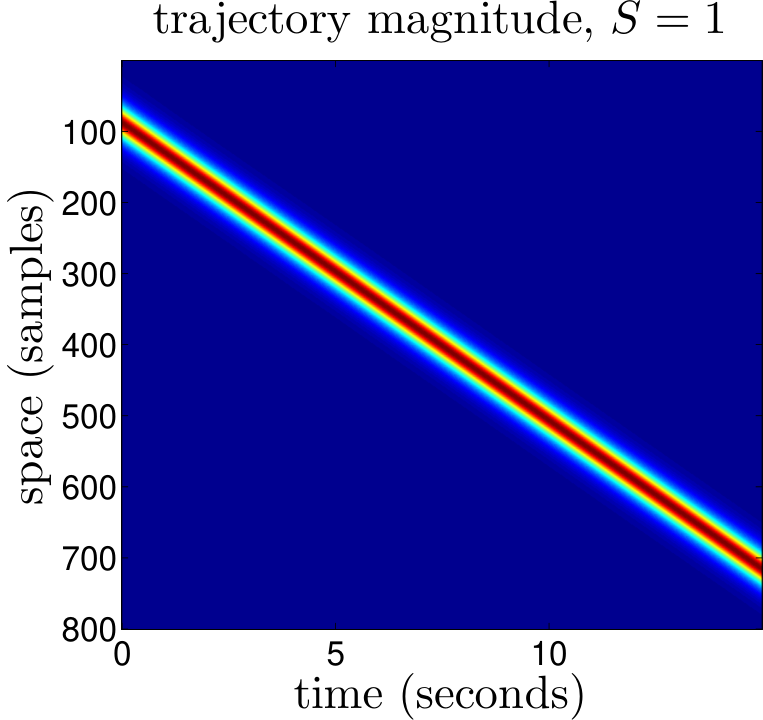
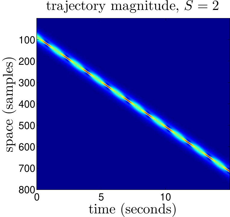
Here, tt denotes the continuous time variable and zz denotes the continuous space variable; utu_{t} denotes the partial derivative of uu with respect to tt and uz​zu_{zz} denotes the second order partial derivative of uu with respect to zz; and we adopt the boundary conditions u→0u\rightarrow 0 as z→±∞z\rightarrow\pm\infty. Adapting the construction provided in [37, Chapter 19], we sample N=800N=800 points between z=−30z=-30 and z=30z=30 at each time to generate data in ℂN\mathbb{C}^{N}. Data is generated with a time step of 0.020.02 seconds. The evolution of the trajectory over time is shown in Figure 3, which plots the magnitude of the entries of each data vector. The three different plots correspond to three different integer values of a parameter SS which is used in the initial conditions

u⁡(z,0)=S⋅sech​(z+z0)⋅ei​Ω​t.u(z,0)=S\cdot\text{sech}(z+z_{0})\cdot e^{\mbox{i}\Omega t}.

The resulting solutions are known as the SS-soliton solutions (with S=1,2,3S=1,2,3) and have an initial center position z0=23.5z_{0}=23.5 and a drift over time due to the group velocity parameter Ω=π\Omega=\pi.

Refer to caption

Refer to caption Refer to caption

Figure 3: Magnitude of trajectory vectors for the Nonlinear Schrödinger system, with S=1S=1, S=2S=2, and S=3S=3-soliton solutions displayed.

We begin by presenting a specific example involving the S=2S=2-soliton solution. Figure 4(a) plots a random projection99 9 This projection, which is useful for obtaining a generic visualization of the trajectory, is computed by constructing a real-valued 3×N3\times N matrix Ξ\Xi populated with independent zero-mean and unit-variance Gaussian random variables. For each data vector x∈ℂNx\in\mathbb{C}^{N}, we compute Ξ​x\Xi x and preserve the real part of the resulting vector. of the data vectors from ℂN\mathbb{C}^{N} to ℝ3\mathbb{R}^{3}, and Figure 4(b) shows the pairwise distances ‖x−y‖22\|x-y\|^{2}_{2} between all pairs x,y∈ℂNx,y\in\mathbb{C}^{N} on the trajectory. Here, we consider only the final ∼5\sim 5 seconds of the data; the initial ∼10\sim 10 seconds are used for populating delay coordinate vectors when needed.

(a) (b) Refer to caption

(c) (d) Refer to caption

Figure 4: Embedding demonstration for the Nonlinear Schrödinger system, S=2S=2-soliton solution with nonlinear RBF measurement functions. (a) Visualization of data vectors x∈ℂNx\in\mathbb{C}^{N} on the trajectory, projected via a random linear map to ℝ3\mathbb{R}^{3}. Color is used to indicate the time (in seconds) corresponding to each data vector xx. (b) Pairwise distances between all pairs x,y∈ℂNx,y\in\mathbb{C}^{N} on the trajectory. (c) Visualization of the resulting delay coordinate vectors Fhα,T,M​(x)F_{h_{\alpha},T,M}(x), projected via a random linear map to ℝ3\mathbb{R}^{3}. Again, color is used to indicate the time (in seconds) corresponding to each original data vector xx. (d) Pairwise distances ‖Fhα,T,M​(x)−Fhα,T,M​(y)‖22\|F_{h_{\alpha},T,M}(x)-F_{h_{\alpha},T,M}(y)\|^{2}_{2} between all points in the reconstruction space.

In this example, we set T=0.06T=0.06 seconds and M=160M=160. To construct the class ℋ\mathcal{H} of measurement functions, we consider a set of P=50P=50 nonlinear radial basis functions (RBFs), each defined by a center vp∈ℂNv_{p}\in\mathbb{C}^{N} randomly chosen from a ball with radius comparable to the data set. The resulting measurement basis functions take the form hp(x)=e−∥x−vp∥2/2σ2h_{p}(x)=e^{-\|x-v_{p}\|^{2}/2\sigma^{2}}, where σ\sigma is a scaling parameter chosen to be comparable to the norm of a typical data vector.

Figure 4(c) shows a random projection of the resulting delay coordinate vectors Fhα,T,M​(x)F_{h_{\alpha},T,M}(x), where the entries of α\alpha are independent Gaussian random variables with zero mean and unit variance. Figure 4(d) shows the pairwise distances ‖Fhα,T,M​(x)−Fhα,T,M​(y)‖22\|F_{h_{\alpha},T,M}(x)-F_{h_{\alpha},T,M}(y)\|^{2}_{2} between all points in the reconstruction space. Figure 5(a) shows a scatter plot comparing the original distances ‖x−y‖22\|x-y\|_{2}^{2} between points on the trajectory to the corresponding distances ‖Fhα,T,M​(x)−Fhα,T,M​(y)‖22\|F_{h_{\alpha},T,M}(x)-F_{h_{\alpha},T,M}(y)\|_{2}^{2} in the reconstruction space ℝM\mathbb{R}^{M}. The dashed lines have slopes equal to the minimum and maximum observed values of the ratio ‖Fhα,T,M​(x)−Fhα,T,M​(y)‖22/‖x−y‖22\|F_{h_{\alpha},T,M}(x)-F_{h_{\alpha},T,M}(y)\|_{2}^{2}/\|x-y\|_{2}^{2} over all pairs x,y∈ℂNx,y\in\mathbb{C}^{N} on the trajectory. Under a highly stable embedding (and in particular if the left and right hand sides of (21) were comparable to one another), the two lines in Figure 5(a) would have slopes comparable to one another. In this experiment, the ratio of the larger slope to the smaller slope is approximately 8.808.80. Up to some degree of approximation, small pairwise distances remain small, and large pairwise distances remain large.

(a) Refer to caption (b) Refer to caption

(c) Refer to caption (d) Refer to caption

Figure 5: Pairwise distance preservation in the various stages of a delay coordinate embedding, S=2S=2-soliton solution with nonlinear RBF measurement functions.

We can unpack the factors that affect the degree of tightness in this embedding. The careful reader of Appendix A and especially (63) will note that the variability of the ratio ‖Fhα,T,M​(x)−Fhα,T,M​(y)‖22/‖x−y‖22\|F_{h_{\alpha},T,M}(x)-F_{h_{\alpha},T,M}(y)\|_{2}^{2}/\|x-y\|_{2}^{2} is affected, in turn, by the variability of the ratios ‖H⁡(x)−H⁡(y)‖22/‖x−y‖22\|H(x)-H(y)\|_{2}^{2}/\|x-y\|_{2}^{2} (see assumption A.1 in Section 3.1 as well as (61)), ‖XH,T,M−YH,T,M‖F2/‖x−y‖22\|X_{H,T,M}-Y_{H,T,M}\|_{F}^{2}/\|x-y\|_{2}^{2} (see (62)), and ‖Fhα,T,M​(x)−Fhα,T,M​(y)‖22/‖XH,T,M−YH,T,M‖F2\|F_{h_{\alpha},T,M}(x)-F_{h_{\alpha},T,M}(y)\|_{2}^{2}/\|X_{H,T,M}-Y_{H,T,M}\|_{F}^{2} (see (57)). Figures 5(b), (c), and (d) show scatter plots corresponding to these three sets of pairwise distances, respectively. Variability in ‖H⁡(x)−H⁡(y)‖22/‖x−y‖22\|H(x)-H(y)\|_{2}^{2}/\|x-y\|_{2}^{2} can be caused by a large ratio between uHu_{H} and lHl_{H}; the ratio of the slopes in Figure 5(b) is approximately 6.356.35. Variability in ‖XH,T,M−YH,T,M‖F2/‖x−y‖22\|X_{H,T,M}-Y_{H,T,M}\|_{F}^{2}/\|x-y\|_{2}^{2} is affected not only by uHu_{H} and lHl_{H}, but also by σmin\sigma_{\min}, σmax\sigma_{\max}, and geo⁡(𝔸)\operatorname{geo}(\mathbb{A}). The ratio of the slopes in Figure 5(c) is approximately 8.058.05. Variability in ‖Fhα,T,M​(x)−Fhα,T,M​(y)‖22/‖XH,T,M−YH,T,M‖F2\|F_{h_{\alpha},T,M}(x)-F_{h_{\alpha},T,M}(y)\|_{2}^{2}/\|X_{H,T,M}-Y_{H,T,M}\|_{F}^{2} is affected by the stable rank RH,T,M⁡(𝔸)\operatorname{R}_{H,T,M}(\mathbb{A}), which in this example is approximately 5.665.66. The ratio of the slopes in Figure 5(d) is approximately 2.142.14. The tests below further reveal the causes and effects of changing the parameters we have discussed here.

To further our study, we also experiment with the S=1S=1-soliton and S=3S=3-soliton solutions, and we test additional classes ℋ\mathcal{H} of measurement functions. In addition to the RBF kernel already considered, we also take ℋ\mathcal{H} to be the space of all linear functionals on ℂN\mathbb{C}^{N}, as in Section 4.1. We also consider a set of nonlinear monomials of maximum degree KK in NN variables. Any such monomial can be written as hp(x)=x[1]β1×x[2]β2×⋯×x[N]βNh_{p}(x)=x[1]^{\beta_{1}}\times x[2]^{\beta_{2}}\times\cdots\times x[N]^{\beta_{N}} for some {βn}n\{\beta_{n}\}_{n} with ∑nβn≤K\sum_{n}\beta_{n}\leq K. We use a set of P=200P=200 randomly-picked monomials with maximum degree K=3K=3.

With a fixed value of T=0.06T=0.06 seconds, Figure 6(a) plots, as a function of MM, the ratio of the largest and smallest isometry constants corresponding to ‖XH,T,M−YH,T,M‖F2/‖x−y‖22\|X_{H,T,M}-Y_{H,T,M}\|_{F}^{2}/\|x-y\|_{2}^{2}. (In the previous example, this corresponded to the ratio of the slopes in Figure 5(c), which was approximately 8.058.05.) Figure 6(b) shows the corresponding plot for ‖Fhα,T,M​(x)−Fhα,T,M​(y)‖22/‖XH,T,M−YH,T,M‖F2\|F_{h_{\alpha},T,M}(x)-F_{h_{\alpha},T,M}(y)\|_{2}^{2}/\|X_{H,T,M}-Y_{H,T,M}\|_{F}^{2}, and Figure 6(c) shows the corresponding plot for ‖Fhα,T,M​(x)−Fhα,T,M​(y)‖22/‖x−y‖22\|F_{h_{\alpha},T,M}(x)-F_{h_{\alpha},T,M}(y)\|_{2}^{2}/\|x-y\|_{2}^{2}, reflecting the tightness of the overall embedding. Figure 6(d) shows the stable rank RH,T,M⁡(𝔸)\operatorname{R}_{H,T,M}(\mathbb{A}) as a function of MM. In these plots, we see several general trends:

  • •

    The overall embedding is generally tightest for the S=1S=1-soliton solution and weakest for the S=3S=3-soliton solution. As illustrated in Figure 3, the complexity of the trajectories generally increases for larger values of SS. For example, the trajectory for S=1S=1 has constant speed, while the instantaneous speed of the trajectory when S=3S=3 varies over a dynamic range of approximately 6.956.95. This variability affects factors such as σmin\sigma_{\min} and σmax\sigma_{\max}, leading to more variability in ‖XH,T,M−YH,T,M‖F2/‖x−y‖22\|X_{H,T,M}-Y_{H,T,M}\|_{F}^{2}/\|x-y\|_{2}^{2} as shown in Figure 6(a). There is relatively little effect of SS on ‖Fhα,T,M​(x)−Fhα,T,M​(y)‖22/‖XH,T,M−YH,T,M‖F2\|F_{h_{\alpha},T,M}(x)-F_{h_{\alpha},T,M}(y)\|_{2}^{2}/\|X_{H,T,M}-Y_{H,T,M}\|_{F}^{2} as shown in Figure 6(b).

  • •

    The linear measurement functions generally result in the tightest embeddings; partly this is due to the fact that lH=uH=1l_{H}=u_{H}=1 in the linear case. The nonlinear monomial functions produce the loosest embeddings. However, the nonlinear RBF functions perform nearly as well as the linear functions.

  • •

    In general, as MM increases, the stable rank increases RH,T,M⁡(𝔸)\operatorname{R}_{H,T,M}(\mathbb{A}), which reduces the variability of ‖Fhα,T,M​(x)−Fhα,T,M​(y)‖22/‖XH,T,M−YH,T,M‖F2\|F_{h_{\alpha},T,M}(x)-F_{h_{\alpha},T,M}(y)\|_{2}^{2}/\|X_{H,T,M}-Y_{H,T,M}\|_{F}^{2} and thus of the overall embedding ‖Fhα,T,M​(x)−Fhα,T,M​(y)‖22/‖x−y‖22\|F_{h_{\alpha},T,M}(x)-F_{h_{\alpha},T,M}(y)\|_{2}^{2}/\|x-y\|_{2}^{2}. This is as expected in light of Theorem 3.1.

(a) (b)

(c) (d)

(e) (f)

Figure 6: Embedding demonstration for the Nonlinear Schrödinger system, including the S=1S=1, S=2S=2, and S=3S=3-soliton solutions and various linear and nonlinear measurement functions. (a)–(d) TT fixed to 0.060.06 seconds. (e)–(f) M​TMT fixed to 9.69.6 seconds.

Finally, over a fixed total delay of 9.69.6 seconds, we experiment with a range of MM values. In each case, we choose T=9.6/MT=9.6/M. Results are shown in Figure 6(e),(f). These results show that, over this total amount of time it is not necessary to sample densely in time; moderately small values of MM (around 4040), corresponding to moderately large values of TT (around 0.240.24 seconds) lead to delay coordinate embeddings with a reasonable degree of tightness.

5 Conclusions and Open Problems

The main result of this paper extends Takens’ celebrated embedding theorem to provide conditions when a delay-coordinate map can provide a stable embedding of a dynamical system attractor. Given the prevalence of these techniques in nonlinear time-series analysis, this result provides a much needed theoretical justification of their numerical performance in the presence of real-world imperfections such as noise and quantization. While the conditions of this result are restrictive and it may not always be possible to meet them in practice, there is significant value in knowing for which scenarios one can guarantee a given quality level of the embedding. In fact, researchers have informally conjectured that instability issues may limit the performance of numerical techniques based on delay-coordinate mapping without the theoretical foundations to examine this issue formally (e.g., see the discussion regarding Takens’ theorem in the Supporting Online Material of [31]). The examination of our results has also led to new and insightful interpretations of classical (generally heuristic) techniques for selecting parameters such as the sampling time and number of delays.

Building on these results, there appears to be no shortage of interesting directions for future work. For example:

  • •

    Remark 3.3 and Table 1 provide a recipe for choosing the sampling interval TT and the number of delays MM in delay-coordinate mapping. It is of interest to experimentally validate this procedure and perhaps find alternatives with lower computational complexity.

  • •

    An open question is whether it is possible to improve (increase) the stable rank of a dynamical system (and hence improve the quality of delay-coordinate mapping) by optimizing over the choice of scalar measurement functions. While we suspect that answer is negative, a rigorous study of this topic does not currently exist.

  • •

    A remaining technical challenge is the role of rch​(𝔸H,T,M)\mbox{rch}(\mathbb{A}_{H,T,M}) (reach of the “trajectory attractor”) in Theorem 3.1 (also see (14)). We suspect that rch​(𝔸H,T,M)\mbox{rch}(\mathbb{A}_{H,T,M}) can be expressed entirely in terms of rch​(𝔸)\mbox{rch}(\mathbb{A}) (and TT, MM, and basis functions {hp}\{h_{p}\}). Such an expression will substantially simplify and clarify Theorem 3.1 but has remained elusive despite our efforts.

  • •

    While multivariate time-series have been occasionally discussed in the literature (e.g., [16]), as with our work, most treatments of delay-coordinate maps are restricted to a single scalar measurement function. An open question is how the presence of multiple measurement functions (producing diverse observations at each sampling time step) would affect the stability of the attractor embedding.

Acknowledgments

AE and MBW acknowledge Liz Bradley at CU Boulder for helpful discussions. AE also thanks Joshua Garland. Part of this research was conducted when AE was a graduate fellow at the Statistical and Applied Mathematical Sciences Institute (SAMSI) and later a visitor at the Institute for Computational and Experimental Research in Mathematics (ICERM). AE is grateful for their hospitality and kindness.

Appendix A Proof of Theorem 3.1 (Stable Takens’ Theorem)

We reserve the letters C,C1,C2,⋯C,C_{1},C_{2},\cdots to represent universal positive constants. We adopt the following (semi-)order: a≲ba\lesssim b means that there is an absolute constant such that a≤\Cr​n​o​t​a​t​i​o​n​1​ba\leq\Cr{notation1}b. If, instead of being an absolute constant, \Cr​n​o​t​a​t​i​o​n​1=\Cr​n​o​t​a​t​i​o​n​1​(θ)\Cr{notation1}=\Cr{notation1}(\theta) depends on some parameter θ\theta, we write a≲θba\lesssim_{\theta}b. Of course, a≳ba\gtrsim b and a≳θba\gtrsim_{\theta}b are defined similarly. Occasionally, we will use the convention that [a:b]=a,a+1,⋯,b[a:b]={a,a+1,\cdots,b} for integers a≤ba\leq b.

Throughout the proof, the dependence on different quantities might be suppressed if there is no ambiguity. Consider x∈𝔸x\in\mathbb{A} and scalar measurement function hα​(⋅)=∑pα⁡[p]⋅hp​(⋅)h_{\alpha}(\cdot)=\sum_{p}\alpha[p]\cdot h_{p}(\cdot) as a linear combination of basis functions. Recall from (11) and (3.1) that the corresponding delay vector can be written as

Fhα,T,M​(x)=XH,T,M⋅α,F_{h_{\alpha},T,M}(x)=X_{H,T,M}\cdot\alpha,
XH,T,M=[H⁡(x)H⁡(ϕT−1​(x))⋯H⁡(ϕT−M+1​(x))]∗∈ℝM×P,X_{H,T,M}=\left[\begin{array}[]{cccc}H(x)&H\left(\phi_{T}^{-1}(x)\right)&\cdots&H\left(\phi_{T}^{-M+1}(x)\right)\end{array}\right]^{*}\in\mathbb{R}^{M\times P}, (35)

and where ϕT:𝔸→𝔸\phi_{T}:\mathbb{A}\rightarrow\mathbb{A} is the flow on the attractor. For a fixed pair of points x,y∈𝔸x,y\in\mathbb{A}, consider the random variable

‖Fhα,T,M​(x)−Fhα,T,M​(y)‖22‖XH,T,M−YH,T,M‖F2=‖XH,T,M⋅α−YH,T,M⋅α‖22‖XH,T,M−YH,T,M‖F2,\frac{\left\|F_{h_{\alpha},T,M}(x)-F_{h_{\alpha},T,M}(y)\right\|_{2}^{2}}{\left\|X_{H,T,M}-Y_{H,T,M}\right\|_{F}^{2}}=\frac{\left\|X_{H,T,M}\cdot\alpha-Y_{H,T,M}\cdot\alpha\right\|_{2}^{2}}{\left\|X_{H,T,M}-Y_{H,T,M}\right\|_{F}^{2}}, (36)

and note that

𝔼⁡[‖Fhα,T,M​(x)−Fhα,T,M​(y)‖22‖XH,T,M−YH,T,M‖F2]=𝔼⁡[‖(XH,T,M−YH,T,M)⋅α‖22]‖XH,T,M−YH,T,M‖F2=1,\mathbb{E}\left[\frac{\left\|F_{h_{\alpha},T,M}(x)-F_{h_{\alpha},T,M}(y)\right\|_{2}^{2}}{\left\|X_{H,T,M}-Y_{H,T,M}\right\|_{F}^{2}}\right]=\frac{\mathbb{E}\left[\left\|\left(X_{H,T,M}-Y_{H,T,M}\right)\cdot\alpha\right\|_{2}^{2}\right]}{\left\|X_{H,T,M}-Y_{H,T,M}\right\|_{F}^{2}}=1,

where the second identity holds because the entries of α∈ℝP\alpha\in\mathbb{R}^{P} are independent and have unit-variance. This suggests that for all pairs of points in 𝔸\mathbb{A}, the ratio in (36) might be close to one. That is, we hope that the following quantity is small with overwhelming probability:

supx,y∈𝔸|‖Fhα,T,M​(x)−Fhα,T,M​(y)‖22‖XH,T,M−YH,T,M‖F2−1|=supZ∈ℨ|‖Z​α‖22−𝔼⁡[‖Z​α‖22]|.\sup_{x,y\in\mathbb{A}}\left|\frac{\left\|F_{h_{\alpha},T,M}(x)-F_{h_{\alpha},T,M}(y)\right\|_{2}^{2}}{\left\|X_{H,T,M}-Y_{H,T,M}\right\|_{F}^{2}}-1\right|=\sup_{Z\in\mathfrak{Z}}\left|\left\|Z\alpha\right\|_{2}^{2}-\mathbb{E}\left[\left\|Z\alpha\right\|_{2}^{2}\right]\right|. (37)

Above, we conveniently set

ℨ:={XH,T,M−YH,T,M‖XH,T,M−YH,T,M‖F:x,y∈𝔸}⊂ℝM×P.\mathfrak{Z}:=\left\{\frac{X_{H,T,M}-Y_{H,T,M}}{\left\|X_{H,T,M}-Y_{H,T,M}\right\|_{F}}\,:\,x,y\in\mathbb{A}\right\}\subset\mathbb{R}^{M\times P}. (38)

To control the supremum in (37), we invoke a recent result by Krahmer et al.

Proposition A.1.

[35, Theorem 3.1] For integers MM and PP, let ℨ⊂ℝM×P\mathfrak{Z}\subset\mathbb{R}^{M\times P} be a collection of matrices. Moreover, let α∈ℝP\alpha\in\mathbb{R}^{P} be a random vector whose entries are independent zero-mean, unit-variance random variables with subgaussian norm of θ\theta. Set

dF​(ℨ)=supZ∈ℨ‖Z‖F,d2​(ℨ)=supZ∈ℨ‖Z‖,d_{F}(\mathfrak{Z})=\sup_{Z\in\mathfrak{Z}}\|Z\|_{F},\qquad d_{2}(\mathfrak{Z})=\sup_{Z\in\mathfrak{Z}}\|Z\|,

where ∥⋅∥F\|\cdot\|_{F} and ∥⋅∥\|\cdot\| stand for the Frobenius and spectral norms, respectively. Also let γ2(ℨ,∥⋅∥)\gamma_{2}(\mathfrak{Z},\|\cdot\|) be the Gaussian width of ℨ\mathfrak{Z} with respect to the spectral metric, and define

E1:=γ2(ℨ,∥⋅∥)⋅(γ2(ℨ,∥⋅∥)+dF(ℨ))+dF(ℨ)⋅d2(ℨ),E_{1}:=\gamma_{2}\left(\mathfrak{Z},\|\cdot\|\right)\cdot\left(\gamma_{2}\left(\mathfrak{Z},\|\cdot\|\right)+d_{F}(\mathfrak{Z})\right)+d_{F}(\mathfrak{Z})\cdot d_{2}(\mathfrak{Z}),
E2:=d22​(ℨ),E_{2}:=d_{2}^{2}(\mathfrak{Z}),
E3:=d2(ℨ)⋅(γ2(ℨ,∥⋅∥)+dF(ℨ)).E_{3}:=d_{2}(\mathfrak{Z})\cdot\left(\gamma_{2}\left(\mathfrak{Z},\|\cdot\|\right)+d_{F}(\mathfrak{Z})\right).

Then, for arbitrary v>0v>0, it holds that

ℙ[supZ∈ℨ|‖Zα‖22−𝔼[‖Zα‖22]|>(θ)⋅E1+v]≤2exp(−(θ)⋅min[vE2,v2E32]),\mathbb{P}\left[\sup_{Z\in\mathfrak{Z}}\left|\left\|Z\alpha\right\|_{2}^{2}-\mathbb{E}\left[\left\|Z\alpha\right\|_{2}^{2}\right]\right|>(\theta)\cdot E_{1}+v\right]\leq 2\exp\left(-(\theta)\cdot\min\left[\frac{v}{E_{2}},\frac{v^{2}}{E_{3}^{2}}\right]\right),

where \Cr​K​r​a​h​m​e​r​(θ)\Cr{Krahmer}(\theta) and \Cr​K​r​a​h​m​e​r​2​(θ)\Cr{Krahmer2}(\theta) depend only on θ\theta.

Without dwelling too much on the concept of Gaussian width above, we recall the following well-known relation [60]:

γ2(ℨ,∥⋅∥)≲∫0∞log(#(ℨ,∥⋅∥,s))ds.\gamma_{2}\left(\mathfrak{Z},\|\cdot\|\right)\lesssim\int_{0}^{\infty}\sqrt{\log\left(\#\left(\mathfrak{Z},\|\cdot\|,s\right)\right)}\,ds. (39)

Above, #(ℨ,∥⋅∥,s)\#(\mathfrak{Z},\|\cdot\|,s) is the covering number of the set ℨ\mathfrak{Z} with respect to the metric ∥⋅∥\|\cdot\| and at scale s>0s>0. That is, #(ℨ,∥⋅∥,s)\#(\mathfrak{Z},\|\cdot\|,s) is the smallest number of balls of radius ss (and with respect to the metric ∥⋅∥\|\cdot\|) needed to cover the set ℨ\mathfrak{Z}. In order to apply Proposition A.1 to (37), we must first calculate dF​(ℨ)d_{F}(\mathfrak{Z}), d2​(ℨ)d_{2}(\mathfrak{Z}), and #(ℨ,∥⋅∥,s)\#(\mathfrak{Z},\|\cdot\|,s) (with ℨ\mathfrak{Z} as in (38)). That, we set out to do next. Observe that

dF​(ℨ)=supZ∈ℨ‖Z‖F=supx,y∈𝔸‖XH,T,M−YH,T,M‖F‖XH,T,M−YH,T,M‖F=1,(see (38))d_{F}\left(\mathfrak{Z}\right)=\sup_{Z\in\mathfrak{Z}}\|Z\|_{F}=\sup_{x,y\in\mathbb{A}}\frac{\left\|X_{H,T,M}-Y_{H,T,M}\right\|_{F}}{\left\|X_{H,T,M}-Y_{H,T,M}\right\|_{F}}=1,\qquad\mbox{(see \eqref{eq:frak Z})} (40)
d2​(ℨ)=supZ∈ℨ‖Z‖=supx,y∈𝔸‖XH,T,M−YH,T,M‖‖XH,T,M−YH,T,M‖F=1RH,T,M⁡(𝔸).(see (17))d_{2}\left(\mathfrak{Z}\right)=\sup_{Z\in\mathfrak{Z}}\|Z\|=\sup_{x,y\in\mathbb{A}}\frac{\left\|X_{H,T,M}-Y_{H,T,M}\right\|}{\left\|X_{H,T,M}-Y_{H,T,M}\right\|_{F}}=\frac{1}{\sqrt{\operatorname{R}_{H,T,M}\left(\mathbb{A}\right)}}.\qquad\mbox{(see \eqref{eq:s rank of h(A)})} (41)

Estimating the covering number of ℨ\mathfrak{Z} is more involved. From the order between norms ∥⋅∥≤∥⋅∥F\|\cdot\|\leq\|\cdot\|_{F}, first deduce that

#(ℨ,∥⋅∥,s)≤#(ℨ,∥⋅∥F,s),∀s>0.\#\left(\mathfrak{Z},\|\cdot\|,s\right)\leq\#\left(\mathfrak{Z},\|\cdot\|_{F},s\right),\qquad\forall s>0. (42)

The covering number on the right hand side above is easier to control, as ℨ⊂ℝM×P\mathfrak{Z}\subset{\mathbb{R}^{M\times P}} is isometric to another (more malleable) object that we denote here with U⁡(𝔸H,T,M)U(\mathbb{A}_{H,T,M}) and define next. Set

xH,T,M=xH,T,M​(x):=vec​(XH,T,M)=[H⁡(x)⋮H⁡(ϕT−M+1​(x))]∈ℝM​P,∀x∈𝔸,x_{H,T,M}=x_{H,T,M}(x):=\mbox{vec}\left(X_{H,T,M}\right)=\left[\begin{array}[]{c}H(x)\\ \vdots\\ H\left(\phi_{T}^{-M+1}(x)\right)\end{array}\right]\in\mathbb{R}^{MP},\qquad\forall x\in\mathbb{A}, (43)
𝔸H,T,M:={xH,T,M:x∈𝔸}⊂ℝM​P.\mathbb{A}_{H,T,M}:=\{x_{H,T,M}\,:\,x\in\mathbb{A}\}\subset\mathbb{R}^{MP}. (44)

Then, let U⁡(𝔸H,T,M)U(\mathbb{A}_{H,T,M}) denote the set of all directions in 𝔸H,T,M\mathbb{A}_{H,T,M}, i.e.,

U(𝔸H,T,M):={xH,T,M−yH,T,M‖xH,T,M−yH,T,M‖2:x,y∈𝔸}⊂§M​P−1,U\left(\mathbb{A}_{H,T,M}\right):=\left\{\frac{x_{H,T,M}-y_{H,T,M}}{\left\|x_{H,T,M}-y_{H,T,M}\right\|_{2}}\,:\,x,y\in\mathbb{A}\right\}\subset\lx@sectionsign^{MP-1}, (45)

where §M​P−1\lx@sectionsign^{MP-1} is the unit sphere in ℝM​P\mathbb{R}^{MP}. Recalling (38), we observe that the pair (ℨ,∥⋅∥F)(\mathfrak{Z},\|\cdot\|_{F}) is isometric to the pair (U(𝔸H,T,M),∥⋅∥2)(U(\mathbb{A}_{H,T,M}),\|\cdot\|_{2}). Thanks to this isometry, we may continue to simplify (42) by writing that

#(ℨ,∥⋅∥,s)\displaystyle\#\left(\mathfrak{Z},\|\cdot\|,s\right) ≤#(ℨ,∥⋅∥F,s)\displaystyle\leq\#\left(\mathfrak{Z},\|\cdot\|_{F},s\right)
=#(U(𝔸H,T,M),∥⋅∥2,s).\displaystyle=\#\left(U\left(\mathbb{A}_{H,T,M}\right),\|\cdot\|_{2},s\right). (46)

Next, we estimate the covering number of U⁡(𝔸H,T,M)U(\mathbb{A}_{H,T,M}). Recall that the attractor 𝔸⊂ℝN\mathbb{A}\subset\mathbb{R}^{N} is a well-behaved manifold and the flow ϕT​(⋅)\phi_{T}(\cdot) is a diffeomorphism on 𝔸\mathbb{A}. Not surprisingly, then, 𝔸H,T,M\mathbb{A}_{H,T,M} (defined in (44)) too is a well-behaved manifold whose geometrical attributes can be expressed in terms of those of 𝔸\mathbb{A}. This observation is formalized next and proved in Appendix B.

Lemma A.1.

Recall the attractor 𝔸⊂ℝN\mathbb{A}\subset\mathbb{R}^{N}, and the flow ϕT:𝔸→𝔸\phi_{T}:\mathbb{A}\rightarrow\mathbb{A}, which by assumption is a diffeomorphism on 𝔸\mathbb{A}. Let D​ϕT​(x):𝕋x​𝔸→𝕋ϕT​(x)​𝔸D\phi_{T}(x):\mathbb{T}_{x}\mathbb{A}\rightarrow\mathbb{T}_{\phi_{T}(x)}\mathbb{A} be the derivative of the flow at x∈𝔸x\in\mathbb{A} (see Section 2.3). The linear map D​ϕT​(x)D\phi_{T}(x) may be identified with a dim⁡(𝔸)×dim⁡(𝔸)\operatorname{dim}(\mathbb{A})\times\operatorname{dim}(\mathbb{A}) matrix. Assume that the singular values of this matrix belong to some interval [σmin,σmax]⊂(0,∞)[\sigma_{\min},\sigma_{\max}]\subset(0,\infty). Lastly, recall the properties of the map H⁡(⋅)H(\cdot) listed in Section 3.1.

Then, 𝔸H,T,M⊂ℝM​P\mathbb{A}_{H,T,M}\subset\mathbb{R}^{MP}, as specified in (44), is a bounded, boundary-less, and smooth submanifold of ℝM​P\mathbb{R}^{MP} with dim⁡(𝔸H,T,M)=dim⁡(𝔸)\operatorname{dim}\left(\mathbb{A}_{H,T,M}\right)=\operatorname{dim}(\mathbb{A}) . Moreover,

ηmindim⁡(𝔸)​σmax−2M⋅dim(𝔸)−1σmax−2⋅dim(𝔸)−1⋅vol⁡(𝔸)≤vol⁡(𝔸H,T,M)≤ηmaxdim⁡(𝔸)​σmin−2M⋅dim(𝔸)−1σmin−2⋅dim(𝔸)−1⋅vol⁡(𝔸).\eta_{\min}^{\operatorname{dim}(\mathbb{A})}\sqrt{\frac{\sigma_{\max}^{-2M\cdot\operatorname{dim}(\mathbb{A})}-1}{\sigma_{\max}^{-2\cdot\operatorname{dim}(\mathbb{A})}-1}}\cdot\operatorname{vol}\left(\mathbb{A}\right)\leq\operatorname{vol}\left(\mathbb{A}_{H,T,M}\right)\leq\eta_{\max}^{\operatorname{dim}(\mathbb{A})}\sqrt{\frac{\sigma_{\min}^{-2M\cdot\operatorname{dim}(\mathbb{A})}-1}{\sigma_{\min}^{-2\cdot\operatorname{dim}(\mathbb{A})}-1}}\cdot\operatorname{vol}\left(\mathbb{A}\right).

The above lemma controls the geometric properties of U⁡(𝔸H,T,M)U(\mathbb{A}_{H,T,M})—its dimension and volume. By substituting these estimates into Lemma 15 of [23], we can in turn control the covering number of U⁡(𝔸H,T,M)U(\mathbb{A}_{H,T,M}) by writing that

#(U(𝔸H,T,M),∥⋅∥2,s)\displaystyle\#\left(U\left(\mathbb{A}_{H,T,M}\right),\|\cdot\|_{2},s\right)
≤2​(6.12​dim⁡(𝔸H,T,M)s2)2⋅dim⁡(𝔸H,T,M)\displaystyle\leq 2\left(\frac{6.12\sqrt{\operatorname{dim}\left(\mathbb{A}_{H,T,M}\right)}}{s^{2}}\right)^{2\cdot\operatorname{dim}\left(\mathbb{A}_{H,T,M}\right)}
⋅(vol⁡(𝔸H,T,M)rch⁡(𝔸H,T,M)dim⁡(𝔸H,T,M))2(invoke [23, Lemma 15])\displaystyle\qquad\cdot\left(\frac{\operatorname{vol}\left(\mathbb{A}_{H,T,M}\right)}{\operatorname{rch}\left(\mathbb{A}_{H,T,M}\right)^{\operatorname{dim}(\mathbb{A}_{H,T,M})}}\right)^{2}\qquad\mbox{(invoke \cite[cite]{[\@@bibref{}{Eftekhari2015}{}{}, Lemma 15]})}
≤2​(6.12​dim⁡(𝔸)s2)2⋅dim⁡(𝔸)⋅ηmax2⋅dim⁡(𝔸)\displaystyle\leq 2\left(\frac{6.12\sqrt{\operatorname{dim}\left(\mathbb{A}\right)}}{s^{2}}\right)^{2\cdot\operatorname{dim}\left(\mathbb{A}\right)}\cdot\eta_{\max}^{2\cdot\operatorname{dim}(\mathbb{A})}
⋅σmin−2M⋅dim(𝔸)−1σmin−2⋅dim(𝔸)−1⋅(vol⁡(𝔸)rch⁡(𝔸H,T,M)dim⁡(𝔸))2,(invoke Lemma A.1)\displaystyle\qquad\cdot\frac{\sigma_{\min}^{-2M\cdot\operatorname{dim}(\mathbb{A})}-1}{\sigma_{\min}^{-2\cdot\operatorname{dim}(\mathbb{A})}-1}\cdot\left(\frac{\operatorname{vol}\left(\mathbb{A}\right)}{\operatorname{rch}\left(\mathbb{A}_{H,T,M}\right)^{\operatorname{dim}(\mathbb{A})}}\right)^{2},\,\mbox{(invoke Lemma \ref{lemma:props of A_h,M,T})}

which holds for any s≤12s\leq\frac{1}{2}, and under the mild assumption that the volume of 𝔸\mathbb{A} is sufficiently large:

vol⁡(𝔸H,T,M)rch⁡(𝔸H,T,M)dim⁡(𝔸H,T,M)\displaystyle\frac{\operatorname{vol}\left(\mathbb{A}_{H,T,M}\right)}{\operatorname{rch}\left(\mathbb{A}_{H,T,M}\right)^{\operatorname{dim}\left(\mathbb{A}_{H,T,M}\right)}} ≥ηmindim⁡(𝔸)​σmax−2M⋅dim(𝔸)−1σmax−2⋅dim(𝔸)−1⋅vol⁡(𝔸)rch⁡(𝔸H,T,M)dim⁡(𝔸)\displaystyle\geq\eta_{\min}^{\operatorname{dim}(\mathbb{A})}\sqrt{\frac{\sigma_{\max}^{-2M\cdot\operatorname{dim}(\mathbb{A})}-1}{\sigma_{\max}^{-2\cdot\operatorname{dim}(\mathbb{A})}-1}}\cdot\frac{\operatorname{vol}\left(\mathbb{A}\right)}{\operatorname{rch}\left(\mathbb{A}_{H,T,M}\right)^{\operatorname{dim}\left(\mathbb{A}\right)}}
≥(212​dim⁡(𝔸H,T,M))dim⁡(𝔸H,T,M)\displaystyle\geq\left(\frac{21}{2\sqrt{\operatorname{dim}\left(\mathbb{A}_{H,T,M}\right)}}\right)^{\operatorname{dim}\left(\mathbb{A}_{H,T,M}\right)}
=(212​dim⁡(𝔸))dim⁡(𝔸).\displaystyle=\left(\frac{21}{2\sqrt{\operatorname{dim}\left(\mathbb{A}\right)}}\right)^{\operatorname{dim}\left(\mathbb{A}\right)}.

In light of (46), we conclude that

#(ℨ,∥⋅∥,s)≤2(6.12​dim⁡(𝔸)s2)2⋅dim⁡(𝔸)ηmax2⋅dim⁡(𝔸)σmin−2M⋅dim(𝔸)−1σmin−2⋅dim(𝔸)−1(vol⁡(𝔸)rch⁡(𝔸H,T,M)dim⁡(𝔸))2,\#\left(\mathfrak{Z},\|\cdot\|,s\right)\leq 2\left(\frac{6.12\sqrt{\operatorname{dim}\left(\mathbb{A}\right)}}{s^{2}}\right)^{2\cdot\operatorname{dim}\left(\mathbb{A}\right)}\eta_{\max}^{2\cdot\operatorname{dim}(\mathbb{A})}\frac{\sigma_{\min}^{-2M\cdot\operatorname{dim}(\mathbb{A})}-1}{\sigma_{\min}^{-2\cdot\operatorname{dim}(\mathbb{A})}-1}\left(\frac{\operatorname{vol}\left(\mathbb{A}\right)}{\operatorname{rch}\left(\mathbb{A}_{H,T,M}\right)^{\operatorname{dim}(\mathbb{A})}}\right)^{2},

and we denote the right hand side by

(Δs)4⋅dim⁡(𝔸).\left(\frac{\Delta}{s}\right)^{4\cdot\operatorname{dim}(\mathbb{A})}. (47)

The above bound holds for every s≤12s\leq\frac{1}{2}, and as long as

vol⁡(𝔸)1dim⁡(𝔸)rch⁡(𝔸H,T,M)\displaystyle\frac{\operatorname{vol}\left(\mathbb{A}\right)^{\frac{1}{\operatorname{dim}(\mathbb{A})}}}{\operatorname{rch}\left(\mathbb{A}_{H,T,M}\right)} ≥ηmin−1​(σmax−2M⋅dim(𝔸)−1σmax−2⋅dim(𝔸)−1)−12⋅dim⁡(𝔸)⋅212​dim⁡(𝔸).\displaystyle\geq\eta_{\min}^{-1}\left(\frac{\sigma_{\max}^{-2M\cdot\operatorname{dim}(\mathbb{A})}-1}{\sigma_{\max}^{-2\cdot\operatorname{dim}(\mathbb{A})}-1}\right)^{-\frac{1}{2\cdot\operatorname{dim}(\mathbb{A})}}\cdot\frac{21}{2\sqrt{\operatorname{dim}\left(\mathbb{A}\right)}}. (48)

With the covering number of ℨ\mathfrak{Z} at hand, we now use (39) to control the Gaussian width of ℨ\mathfrak{Z}:

γ2(ℨ,∥⋅∥)\displaystyle\gamma_{2}\left(\mathfrak{Z},\|\cdot\|\right)
≲∫0∞log(#(ℨ,∥⋅∥,s))​𝑑s\displaystyle\lesssim\int_{0}^{\infty}\sqrt{\log\left(\#\left(\mathfrak{Z},\|\cdot\|,s\right)\right)}\,ds
=∫02⋅d2​(ℨ)log(#(ℨ,∥⋅∥,s))ds(from (41): s≥2⋅d2(ℨ)⟹#(ℨ,∥⋅∥,s)=1)\displaystyle=\int_{0}^{2\cdot d_{2}\left(\mathfrak{Z}\right)}\sqrt{\log\left(\#\left(\mathfrak{Z},\|\cdot\|,s\right)\right)}\,ds\qquad\left(\mbox{from \eqref{eq:bnd on d2}: }s\geq 2\cdot d_{2}\left(\mathfrak{Z}\right)\Longrightarrow\#\left(\mathfrak{Z},\|\cdot\|,s\right)=1\right)
≤∫02RH,T,M⁡(𝔸)log(#(ℨ,∥⋅∥,s))ds(see (41))\displaystyle\leq\int_{0}^{\frac{2}{\sqrt{\operatorname{R}_{H,T,M}(\mathbb{A})}}}\sqrt{\log\left(\#\left(\mathfrak{Z},\|\cdot\|,s\right)\right)}\,ds\qquad\mbox{(see \eqref{eq:bnd on d2})}
≤4⋅dim⁡(𝔸)∫02RH,T,M⁡(𝔸)log⁡(Δs)ds(see (47))\displaystyle\leq\sqrt{4\cdot\operatorname{dim}(\mathbb{A})}\int_{0}^{\frac{2}{\sqrt{\operatorname{R}_{H,T,M}(\mathbb{A})}}}\sqrt{\log\left(\frac{\Delta}{s}\right)}\,ds\qquad\left(\mbox{see \eqref{eq:bnd on co no of Z}}\right)
≤4⋅dim⁡(𝔸)⋅(4RH,T,M⁡(𝔸))14\displaystyle\leq\sqrt{4\cdot\operatorname{dim}(\mathbb{A})}\cdot\left(\frac{4}{\operatorname{R}_{H,T,M}(\mathbb{A})}\right)^{\frac{1}{4}}
∫02RH,T,M⁡(𝔸)log⁡(Δs)​𝑑s(∫0af⁡(s)​𝑑s≤a⋅∫0af⁡(s)​𝑑s)\displaystyle\quad\sqrt{\int_{0}^{\frac{2}{\sqrt{\operatorname{R}_{H,T,M}(\mathbb{A})}}}\log\left(\frac{\Delta}{s}\right)\,ds}\quad\left(\int_{0}^{a}\sqrt{f(s)}\,ds\leq\sqrt{a\cdot\int_{0}^{a}f(s)\,ds}\right)
≤4⋅dim⁡(𝔸)⋅(4RH,T,M⁡(𝔸))14​∫02RH,T,M⁡(𝔸)log⁡(1+Δs)​𝑑s\displaystyle\leq\sqrt{4\cdot\operatorname{dim}(\mathbb{A})}\cdot\left(\frac{4}{\operatorname{R}_{H,T,M}(\mathbb{A})}\right)^{\frac{1}{4}}\sqrt{\int_{0}^{\frac{2}{\sqrt{\operatorname{R}_{H,T,M}(\mathbb{A})}}}\log\left(1+\frac{\Delta}{s}\right)\,ds}
≤4⋅dim⁡(𝔸)⋅(4RH,T,M⁡(𝔸))14⋅4RH,T,M⁡(𝔸)\displaystyle\leq\sqrt{4\cdot\operatorname{dim}(\mathbb{A})}\cdot\left(\frac{4}{\operatorname{R}_{H,T,M}(\mathbb{A})}\right)^{\frac{1}{4}}\cdot\sqrt{\frac{4}{\sqrt{\operatorname{R}_{H,T,M}(\mathbb{A})}}}
⋅log⁡(1+Δ​RH,T,M⁡(𝔸)2)(∫0alog(1+bs)ds≤2a⋅log(1+ba), if a≤b)\displaystyle\,\cdot\sqrt{\log\left(1+\frac{\Delta\sqrt{\operatorname{R}_{H,T,M}(\mathbb{A})}}{2}\right)}\quad\left(\int_{0}^{a}\log\left(1+\frac{b}{s}\right)\,ds\leq 2a\cdot\log\left(1+\frac{b}{a}\right),\mbox{ if }a\leq b\right)
≤8dim⁡(𝔸)RH,T,M⁡(𝔸)⋅log⁡(Δ​RH,T,M⁡(𝔸))(log(1+a)≤2log(a),∀a≥2)\displaystyle\leq 8\sqrt{\frac{\operatorname{dim}(\mathbb{A})}{\operatorname{R}_{H,T,M}(\mathbb{A})}\cdot\log\left(\Delta\sqrt{\operatorname{R}_{H,T,M}(\mathbb{A})}\right)}\qquad\left(\log(1+a)\leq 2\log(a),\,\forall a\geq 2\right) (49)

and, by simplifying the last line,

γ2(𝒵,∥⋅∥)\displaystyle\gamma_{2}\left(\mathcal{Z},\|\cdot\|\right)
≲dim⁡(𝔸)RH,T,M⁡(𝔸)\displaystyle\lesssim\sqrt{\frac{\operatorname{dim}(\mathbb{A})}{\operatorname{R}_{H,T,M}(\mathbb{A})}}
⋅log⁡(dim⁡(𝔸)​ηmax​(σmin−2M⋅dim(𝔸)−1σmin−2⋅dim(𝔸)−1)12⋅dim⁡(𝔸)​vol⁡(𝔸)1dim⁡(𝔸)rch⁡(𝔸H,T,M)⋅RH,T,M⁡(𝔸)).(see (47))\displaystyle\cdot\sqrt{\log\left(\sqrt{\operatorname{dim}(\mathbb{A})}\eta_{\max}\left(\frac{\sigma_{\min}^{-2M\cdot\operatorname{dim}(\mathbb{A})}-1}{\sigma_{\min}^{-2\cdot\operatorname{dim}(\mathbb{A})}-1}\right)^{\frac{1}{2\cdot\operatorname{dim}(\mathbb{A})}}\frac{\operatorname{vol}(\mathbb{A})^{\frac{1}{\operatorname{dim}(\mathbb{A})}}}{\operatorname{rch}(\mathbb{A}_{H,T,M})}\cdot\operatorname{R}_{H,T,M}(\mathbb{A})\right)}.\,\mbox{(see \eqref{eq:bnd on co no of Z}) } (50)

For the fifth and tenth lines to hold, we must impose that

RH,T,M⁡(𝔸)≥16⋅max⁡(1,Δ−2).\operatorname{R}_{H,T,M}(\mathbb{A})\geq 16\cdot\max\left(1,\Delta^{-2}\right). (51)

For (51) to hold, it actually suffices to assume that

RH,T,M⁡(𝔸)≳1,\operatorname{R}_{H,T,M}(\mathbb{A})\gtrsim 1, (52)
dim⁡(𝔸)⋅ηmax⋅(σmin−2M⋅dim(𝔸)−1σmin−2⋅dim(𝔸)−1)12⋅dim⁡(𝔸)⋅vol⁡(𝔸)1dim⁡(𝔸)rch⁡(𝔸H,T,M)≳1.(see (47))\sqrt{\operatorname{dim}(\mathbb{A})}\cdot\eta_{\max}\cdot\left(\frac{\sigma_{\min}^{-2M\cdot\operatorname{dim}(\mathbb{A})}-1}{\sigma_{\min}^{-2\cdot\operatorname{dim}(\mathbb{A})}-1}\right)^{\frac{1}{2\cdot\operatorname{dim}(\mathbb{A})}}\cdot\frac{\operatorname{vol}(\mathbb{A})^{\frac{1}{\operatorname{dim}(\mathbb{A})}}}{\operatorname{rch}(\mathbb{A}_{H,T,M})}\gtrsim 1.\qquad\mbox{(see \eqref{eq:bnd on co no of Z})} (53)

We note that (53) is guaranteed to hold if (48) (which appears in the theorem statement as (20)) holds. Given the estimates of dF​(ℨ)d_{F}(\mathfrak{Z}), d2​(ℨ)d_{2}(\mathfrak{Z}), and γ2(ℨ,∥⋅∥)\gamma_{2}(\mathfrak{Z},\|\cdot\|) (see (40-41) and (50)), we are now in position to apply Proposition A.1 to ℨ\mathfrak{Z} (specified in (38)). For δ,ρ∈(0,1)\delta,\rho\in(0,1), assume that

RH,T,M⁡(𝔸)\displaystyle\operatorname{R}_{H,T,M}(\mathbb{A}) ≳δ−2⋅dim⁡(𝔸)⋅log⁡(dim⁡(𝔸)⋅ηmax⋅(σmin−2M⋅dim(𝔸)−1σmin−2⋅dim(𝔸)−1)12⋅dim⁡(𝔸)⋅vol⁡(𝔸)1dim⁡(𝔸)rch⁡(𝔸H,T,M)CLOSE\displaystyle\gtrsim\delta^{-2}\cdot\operatorname{dim}(\mathbb{A})\cdot\log\Bigg(\sqrt{\operatorname{dim}(\mathbb{A})}\cdot\eta_{\max}\cdot\left(\frac{\sigma_{\min}^{-2M\cdot\operatorname{dim}(\mathbb{A})}-1}{\sigma_{\min}^{-2\cdot\operatorname{dim}(\mathbb{A})}-1}\right)^{\frac{1}{2\cdot\operatorname{dim}(\mathbb{A})}}\cdot\frac{\operatorname{vol}(\mathbb{A})^{\frac{1}{\operatorname{dim}(\mathbb{A})}}}{\operatorname{rch}(\mathbb{A}_{H,T,M})}
OPENRH,T,M⁡(𝔸))+δ−2⋅log⁡(1ρ).\displaystyle\qquad\operatorname{R}_{H,T,M}(\mathbb{A})\Bigg)+\delta^{-2}\cdot\log\left(\frac{1}{\rho}\right). (54)

Under this assumption, we obtain that

dF​(ℨ)\displaystyle d_{F}(\mathfrak{Z}) =1,(see (40))\displaystyle=1,\qquad\mbox{(see \eqref{eq:bnd on dF})}
d2​(ℨ)\displaystyle d_{2}(\mathfrak{Z}) =1RH,T,M⁡(𝔸)≲δ⋅(log⁡(1ρ))−12,(see (41))\displaystyle=\frac{1}{\sqrt{\operatorname{R}_{H,T,M}(\mathbb{A})}}\lesssim\delta\cdot\left(\log\left(\frac{1}{\rho}\right)\right)^{-\frac{1}{2}},\qquad\mbox{(see \eqref{eq:bnd on d2})}
γ2(ℨ,∥⋅∥)\displaystyle\gamma_{2}\left(\mathfrak{Z},\|\cdot\|\right) ≲δ.(see (50))\displaystyle\lesssim\delta.\quad\mbox{(see \eqref{eq:bnd on gamma2})}

Subsequently, the quantities E1E_{1}, E2E_{2}, and E3E_{3} in Proposition A.1 may be bounded as

E1\displaystyle E_{1} ≲δ⋅(δ+1)+δ⋅(log⁡(1ρ))−12≲δ,(ρ<1)\displaystyle\lesssim\delta\cdot(\delta+1)+\delta\cdot\left(\log\left(\frac{1}{\rho}\right)\right)^{-\frac{1}{2}}\lesssim\delta,\qquad\left(\rho<1\right)
E2\displaystyle E_{2} ≲δ2⋅(log⁡(1ρ))−1,\displaystyle\lesssim\delta^{2}\cdot\left(\log\left(\frac{1}{\rho}\right)\right)^{-1},
E3\displaystyle E_{3} ≲δ⋅(log⋅(1ρ))−12⋅(δ+1)≲δ⋅(log⁡(1ρ))−12.\displaystyle\lesssim\delta\cdot\left(\log\cdot\left(\frac{1}{\rho}\right)\right)^{-\frac{1}{2}}\cdot(\delta+1)\lesssim\delta\cdot\left(\log\left(\frac{1}{\rho}\right)\right)^{-\frac{1}{2}}.

We now recall (37), substitute the above quantities into Proposition A.1 with an arbitrary v>0v>0, and finally find that

ℙ[supx,y∈𝔸|‖Fhα,T,M​(x)−Fhα,T,M​(y)‖22‖XH,T,M−YH,T,M‖F2−1|>\CrKrahmer(θ)⋅δ+v]\displaystyle\mathbb{P}\left[\sup_{x,y\in\mathbb{A}}\left|\frac{\left\|F_{h_{\alpha},T,M}(x)-F_{h_{\alpha},T,M}(y)\right\|_{2}^{2}}{\left\|X_{H,T,M}-Y_{H,T,M}\right\|_{F}^{2}}-1\right|>\Cr{Krahmer}(\theta)\cdot\delta+v\right]
=ℙ[supZ∈ℨ|‖Zα‖22−𝔼[‖Zα‖22]|>\CrKrahmer(θ)⋅δ+v](see (37))\displaystyle=\mathbb{P}\left[\sup_{Z\in\mathfrak{Z}}\left|\left\|Z\alpha\right\|_{2}^{2}-\mathbb{E}\left[\left\|Z\alpha\right\|_{2}^{2}\right]\right|>\Cr{Krahmer}(\theta)\cdot\delta+v\right]\qquad\mbox{(see \eqref{eq:goal})}
≤ℙ[supZ∈ℨ|‖Zα‖22−𝔼[‖Zα‖22]|>\CrKrahmer(θ)⋅E1+v](see (A))\displaystyle\leq\mathbb{P}\left[\sup_{Z\in\mathfrak{Z}}\left|\left\|Z\alpha\right\|_{2}^{2}-\mathbb{E}\left[\left\|Z\alpha\right\|_{2}^{2}\right]\right|>\Cr{Krahmer}(\theta)\cdot E_{1}+v\right]\qquad\mbox{(see \eqref{eq:bnds on E123})}
≤2⋅exp(−\CrKrahmer2(θ)⋅min[vE2,v2E32])(see Proposition A.1)\displaystyle\leq 2\cdot\exp\left(-\Cr{Krahmer2}(\theta)\cdot\min\left[\frac{v}{E_{2}},\frac{v^{2}}{E_{3}^{2}}\right]\right)\qquad\mbox{(see Proposition \ref{prop:Krahmer})}
≤2⋅exp(−\Cr​K​r​a​h​m​e​r​2​(θ)δ2⋅log(1ρ)⋅min(v2,v)).(see (A))\displaystyle\leq 2\cdot\exp\left(-\frac{\Cr{Krahmer2}(\theta)}{\delta^{2}}\cdot\log\left(\frac{1}{\rho}\right)\cdot\min\left(v^{2},v\right)\right).\qquad\mbox{(see \eqref{eq:bnds on E123})} (55)

By assigning v=δv=\delta above, we conclude that

ℙ[supx,y∈𝔸|‖Fhα,T,M​(x)−Fhα,T,M​(y)‖22‖XH,T,M−YH,T,M‖F2−1|>(θ)⋅δ]\displaystyle\mathbb{P}\left[\sup_{x,y\in\mathbb{A}}\left|\frac{\left\|F_{h_{\alpha},T,M}(x)-F_{h_{\alpha},T,M}(y)\right\|_{2}^{2}}{\left\|X_{H,T,M}-Y_{H,T,M}\right\|_{F}^{2}}-1\right|>(\theta)\cdot\delta\right]
≤2⋅exp(−\Cr​K​r​a​h​m​e​r​2​(θ)δ2⋅log(1ρ)⋅min(δ2,δ))\displaystyle\leq 2\cdot\exp\left(-\frac{\Cr{Krahmer2}(\theta)}{\delta^{2}}\cdot\log\left(\frac{1}{\rho}\right)\cdot\min\left(\delta^{2},\delta\right)\right)
≤(θ)⋅ρ,(δ<1)\displaystyle\leq(\theta)\cdot\rho,\qquad\left(\delta<1\right) (56)

for \Cr​K​r​a​h​m​e​r​p​(θ)\Cr{Krahmerp}(\theta) and \Cr​K​r​a​h​m​e​r​2​p​(θ)\Cr{Krahmer2p}(\theta) that depend only on θ\theta. Equivalently, if we replace ≳\gtrsim in (54) with ≳θ\gtrsim_{\theta}, we can further simplify the above inequality to read

ℙ[supx,y∈𝔸|‖Fhα,T,M​(x)−Fhα,T,M​(y)‖22‖XH,T,M−YH,T,M‖F2−1|>δ]\displaystyle\mathbb{P}\left[\sup_{x,y\in\mathbb{A}}\left|\frac{\left\|F_{h_{\alpha},T,M}(x)-F_{h_{\alpha},T,M}(y)\right\|_{2}^{2}}{\left\|X_{H,T,M}-Y_{H,T,M}\right\|_{F}^{2}}-1\right|>\delta\right] ≤(θ)⋅ρ,\displaystyle\leq(\theta)\cdot\rho, (57)

for \Cr​K​r​a​h​m​e​r​2​p​p​(θ)\Cr{Krahmer2pp}(\theta) that depend only on θ\theta. Here, ≳θ\gtrsim_{\theta} hides the explicit dependence on θ\theta for convenience. This proves the version of Theorem 3.1 that appears in Remark A.1.

Fix x,y∈𝔸x,y\in\mathbb{A}. We can in fact replace ‖XH,T,M−YH,T,M‖F\|X_{H,T,M}-Y_{H,T,M}\|_{F} above with a more approachable quantity as follows. From (35), recall that

‖XH,T,M−YH,T,M‖F2=∑m=0M−1‖H⁡(ϕT−m​(x))−H⁡(ϕT−m​(y))‖22,\left\|X_{H,T,M}-Y_{H,T,M}\right\|_{F}^{2}=\sum_{m=0}^{M-1}\left\|H\left(\phi_{T}^{-m}(x)\right)-H\left(\phi_{T}^{-m}(y)\right)\right\|_{2}^{2}, (58)

which suggests that we should find a more convenient expression for each summand above. Invoking the assumption in Theorem 3.1 that the spectrum of D​ϕT​(⋅)D\phi_{T}(\cdot) (the derivative of the flow) belongs to some interval [σmin,σmax]∈(0,∞)[\sigma_{\min},\sigma_{\max}]\in(0,\infty), we may easily verify that

σmax−m⋅d𝔸​(x,y)≤d𝔸​(ϕT−m​(x),ϕT−m​(y))≤σmin−m⋅d𝔸​(x,y),\sigma_{\max}^{-m}\cdot d_{\mathbb{A}}\left(x,y\right)\leq d_{\mathbb{A}}\left(\phi_{T}^{-m}(x),\phi_{T}^{-m}(y)\right)\leq\sigma_{\min}^{-m}\cdot d_{\mathbb{A}}\left(x,y\right), (59)

where d𝔸​(⋅,⋅)d_{\mathbb{A}}(\cdot,\cdot) returns the geodesic distance between a pair of points on 𝔸\mathbb{A} (see Section 2.3). To relate the geodesic metric on 𝔸\mathbb{A} to the Euclidean metric in ℝN\mathbb{R}^{N}, we recall the regularity condition (5), from which it follows that

geo⁡(𝔸)−1⋅σmax−m⋅‖x−y‖2≤‖ϕT−m​(x)−ϕT−m​(y)‖2≤geo⁡(𝔸)⋅σmin−m⋅‖x−y‖2.\operatorname{geo}(\mathbb{A})^{-1}\cdot\sigma_{\max}^{-m}\cdot\left\|x-y\right\|_{2}\leq\left\|\phi_{T}^{-m}(x)-\phi_{T}^{-m}(y)\right\|_{2}\leq\operatorname{geo}(\mathbb{A})\cdot\sigma_{\min}^{-m}\cdot\left\|x-y\right\|_{2}. (60)

Next, recalling the bi-Lipschitz property of H⁡(⋅)H(\cdot) in Section 3.1 allows us to update the above relation to read:

lH⋅geo⁡(𝔸)−1⋅σmax−m⋅‖x−y‖2≤‖H⁡(ϕT−m​(x))−H⁡(ϕT−m​(y))‖2≤uH⋅geo⁡(𝔸)⋅σmin−m⋅‖x−y‖2.l_{H}\cdot\operatorname{geo}(\mathbb{A})^{-1}\cdot\sigma_{\max}^{-m}\cdot\left\|x-y\right\|_{2}\leq\left\|H\left(\phi_{T}^{-m}(x)\right)-H\left(\phi_{T}^{-m}(y)\right)\right\|_{2}\leq u_{H}\cdot\operatorname{geo}(\mathbb{A})\cdot\sigma_{\min}^{-m}\cdot\left\|x-y\right\|_{2}. (61)

From (58), it then follows that

lH2⋅geo⁡(𝔸)−2⋅σmax−2​M−1σmax−2−1⋅‖x−y‖22≤‖XH,T,M−YH,T,M‖F2≤uH2⋅geo⁡(𝔸)2⋅σmin−2​M−1σmin2−1⋅‖x−y‖22.l_{H}^{2}\cdot\operatorname{geo}(\mathbb{A})^{-2}\cdot\frac{\sigma_{\max}^{-2M}-1}{\sigma_{\max}^{-2}-1}\cdot\|x-y\|_{2}^{2}\leq\left\|X_{H,T,M}-Y_{H,T,M}\right\|_{F}^{2}\leq u_{H}^{2}\cdot\operatorname{geo}(\mathbb{A})^{2}\cdot\frac{\sigma_{\min}^{-2M}-1}{\sigma_{\min}^{2}-1}\cdot\|x-y\|_{2}^{2}. (62)

In turn, (57) now implies that

(1−δ)⋅lH2⋅geo⁡(𝔸)−2⋅σmax−2​M−1σmax−2−1≤‖Fhα,T,M​(x)−Fhα,T,M​(y)‖22‖x−y‖22(1-\delta)\cdot l_{H}^{2}\cdot\operatorname{geo}(\mathbb{A})^{-2}\cdot\frac{\sigma_{\max}^{-2M}-1}{\sigma_{\max}^{-2}-1}\leq\frac{\left\|F_{h_{\alpha},T,M}(x)-F_{h_{\alpha},T,M}(y)\right\|_{2}^{2}}{\|x-y\|_{2}^{2}} (63)
≤(1+δ)⋅uH2⋅geo⁡(𝔸)2⋅σmin−2​M−1σmin−2−1,\qquad\qquad\qquad\qquad\qquad\leq(1+\delta)\cdot u_{H}^{2}\cdot\operatorname{geo}(\mathbb{A})^{2}\cdot\frac{\sigma_{\min}^{-2M}-1}{\sigma_{\min}^{-2}-1},

except with a probability of at most \Cr​K​r​a​h​m​e​r​2​p​p​(θ)⋅ρ\Cr{Krahmer2pp}(\theta)\cdot\rho. To reiterate, the above relation holds under (54) (with ≳θ\gtrsim_{\theta} rather than ≳\gtrsim), and under the mild assumption that

vol⁡(𝔸)1dim⁡(𝔸)rch⁡(𝔸H,T,M)≳1ηmin​dim⁡(𝔸)⋅(σmax−2M⋅dim(𝔸)−1σmax−2⋅dim(𝔸)−1)−12⋅dim⁡(𝔸).\frac{\operatorname{vol}\left(\mathbb{A}\right)^{\frac{1}{\operatorname{dim}(\mathbb{A})}}}{\operatorname{rch}\left(\mathbb{A}_{H,T,M}\right)}\gtrsim\frac{1}{\eta_{\min}\sqrt{\operatorname{dim}(\mathbb{A})}}\cdot\left(\frac{\sigma_{\max}^{-2M\cdot\operatorname{dim}(\mathbb{A})}-1}{\sigma_{\max}^{-2\cdot\operatorname{dim}(\mathbb{A})}-1}\right)^{-\frac{1}{2\cdot\operatorname{dim}(\mathbb{A})}}. (64)

As our last step, we now remove the stable rank from the right hand side of (54). To accomplish that, we focus on the requirement that

RH,T,M(𝔸)≳θδ−2⋅dim(𝔸)⋅log(RH,T,M(𝔸)).\operatorname{R}_{H,T,M}\left(\mathbb{A}\right)\gtrsim_{\theta}\delta^{-2}\cdot\operatorname{dim}(\mathbb{A})\cdot\log\left(\operatorname{R}_{H,T,M}\left(\mathbb{A}\right)\right). (65)

The Lambert W-function W⁡(⋅)W(\cdot) [41, §4.13] is defined through the relation W⁡(z)⋅eW⁡(z)=zW(z)\cdot e^{W(z)}=z. Strictly speaking, the Lambert W-function is not a function, as it is multi-valued when z<0z<0. In this case, W⁡(z)W(z) denotes the preimage of W⁡(z)⋅eW⁡(z)=zW(z)\cdot e^{W(z)}=z. Then, it is not difficult to verify that the requirement above is equivalent to

RH,T,M(𝔸)≳θe−min⁡W⁡(−δ2dim⁡(𝔸)).\operatorname{R}_{H,T,M}\left(\mathbb{A}\right)\gtrsim_{\theta}e^{-\min W\left(-\frac{\delta^{2}}{\operatorname{dim}(\mathbb{A})}\right)}. (66)

This allows us to rewrite (54) as

RH,T,M⁡(𝔸)\displaystyle\operatorname{R}_{H,T,M}\left(\mathbb{A}\right)
≳θmax[δ−2⋅dim(𝔸)⋅log(ηmaxdim⁡(𝔸)(σmin−2M⋅dim(𝔸)−1σmin−2⋅dim(𝔸)−1)12⋅dim⁡(𝔸)vol⁡(𝔸)1dim⁡(𝔸)rch⁡(𝔸H,T,M))\displaystyle\gtrsim_{\theta}\max\Bigg[\delta^{-2}\cdot\operatorname{dim}(\mathbb{A})\cdot\log\left(\eta_{\max}\sqrt{\operatorname{dim}(\mathbb{A})}\left(\frac{\sigma_{\min}^{-2M\cdot\operatorname{dim}\left(\mathbb{A}\right)}-1}{\sigma_{\min}^{-2\cdot\operatorname{dim}(\mathbb{A})}-1}\right)^{\frac{1}{2\cdot\operatorname{dim}(\mathbb{A})}}\frac{\operatorname{vol}\left(\mathbb{A}\right)^{\frac{1}{\operatorname{dim}(\mathbb{A})}}}{\operatorname{rch}(\mathbb{A}_{H,T,M})}\right)
,e−min⁡W⁡(−δ2dim⁡(𝔸)),δ−2log(1ρ)].\displaystyle\qquad\qquad\qquad,e^{-\min W\left(\frac{-\delta^{2}}{\operatorname{dim}(\mathbb{A})}\right)},\delta^{-2}\log\left(\frac{1}{\rho}\right)\Bigg]. (67)

The proof of Theorem 3.1 is now complete.

Remark A.1.

(Poor geodesic regularity) If the geodesic regularity of the attractor is poor (i.e., if geo⁡(𝔸)\operatorname{geo}(\mathbb{A}) in (5) is large), also, if the singular values have a high ratio (as in a chaotic system), then perhaps the following slightly weaker result is more useful. Theorem 3.1 holds verbatim but with the following replacing (21):

1−δ≤‖Fhα,T,M​(x)−Fhα,T,M​(y)‖F2∑m=0M−1‖H⁡(ϕT−m​(x))−H⁡(ϕT−m​(y))‖22≤1+δ,∀x,y∈𝔸.\displaystyle 1-\delta\leq\frac{\left\|F_{h_{\alpha},T,M}(x)-F_{h_{\alpha},T,M}(y)\right\|_{F}^{2}}{\sum_{m=0}^{M-1}\left\|H\left(\phi^{-m}_{T}(x)\right)-H\left(\phi^{-m}_{T}(y)\right)\right\|_{2}^{2}}\leq 1+\delta,\qquad\forall x,y\in\mathbb{A}. (68)

Appendix B Proof of Lemma A.1

Recall that 𝔸⊂ℝN\mathbb{A}\subset\mathbb{R}^{N} is a bounded, boundary-less, and smooth manifold. Also, both ϕT:𝔸→𝔸\phi_{T}:\mathbb{A}\rightarrow\mathbb{A} and H:𝔸→H⁡(𝔸)H:\mathbb{A}\rightarrow H(\mathbb{A}) are diffeomorphisms. It follows that 𝔸H,T,M⊂ℝM​P\mathbb{A}_{H,T,M}\subset\mathbb{R}^{MP} (defined in (44)) too is a bounded, boundary-less, and smooth manifold, and that dim⁡(𝔸H,T,M)=dim⁡(𝔸)\operatorname{dim}(\mathbb{A}_{H,T,M})=\operatorname{dim}(\mathbb{A}).

As for vol⁡(𝔸H,T,M)\operatorname{vol}(\mathbb{A}_{H,T,M}), we argue as follows. For x∈𝔸x\in\mathbb{A}, let D​H​(x):𝕋x​𝔸→𝕋H⁡(x)​H​(𝔸)DH(x):\mathbb{T}_{x}\mathbb{A}\rightarrow\mathbb{T}_{H(x)}H(\mathbb{A}) be the derivative of H⁡(⋅)H(\cdot) at x∈𝔸x\in\mathbb{A} (see Section 2.3). Each tangent space may be identified with ℝdim⁡(𝔸)\mathbb{R}^{\operatorname{dim}(\mathbb{A})} and, consequently, D​H​(x)DH(x) may be identified with a dim⁡(𝔸)×dim⁡(𝔸)\operatorname{dim}(\mathbb{A})\times\operatorname{dim}(\mathbb{A}) matrix. By assumption, the singular spectrum of D​H​(x)DH(x) belongs to the interval [ηmin,ηmax]⊂(0,∞)[\eta_{\min},\eta_{\max}]\subset(0,\infty) (see Section 3.1). Then, the volume element of 𝔸\mathbb{A} under H⁡(⋅)H(\cdot) deforms as

ηmindim⁡(𝔸)⋅d​vol⁡(x)≤d​vol⁡(H⁡(x))≤ηmaxdim⁡(𝔸)⋅d​vol⁡(x),∀x∈𝔸.\eta_{\min}^{\operatorname{dim}(\mathbb{A})}\cdot d\operatorname{vol}(x)\leq d\operatorname{vol}\left(H(x)\right)\leq\eta_{\max}^{\operatorname{dim}(\mathbb{A})}\cdot d\operatorname{vol}(x),\qquad\forall x\in\mathbb{A}. (69)

Similarly, let D​ϕT​(x):𝕋x​𝔸→𝕋ϕ⁡(x)​𝔸D\phi_{T}(x):\mathbb{T}_{x}\mathbb{A}\rightarrow\mathbb{T}_{\phi(x)}\mathbb{A} be the derivative of the flow at x∈𝔸x\in\mathbb{A}. By assumption, the singular spectrum of D​ϕ​(x)D\phi(x) belongs to the interval [σmin,σmax]⊂(0,∞)[\sigma_{\min},\sigma_{\max}]\subset(0,\infty). Then, the volume element of 𝔸\mathbb{A} under ϕT−1​(⋅)\phi_{T}^{-1}(\cdot) deforms as

σmax−dim⁡(𝔸)⋅d​vol⁡(x)≤d​vol⁡(ϕT−1​(x))≤σmin−dim⁡(𝔸)⋅d​vol⁡(x),∀x∈𝔸.\sigma_{\max}^{-\operatorname{dim}(\mathbb{A})}\cdot d\operatorname{vol}(x)\leq d\operatorname{vol}\left(\phi_{T}^{-1}(x)\right)\leq{\sigma_{\min}^{-\operatorname{dim}(\mathbb{A})}}\cdot d\operatorname{vol}(x),\qquad\forall x\in\mathbb{A}. (70)

Predicated on the above observations, we have that

vol⁡(𝔸H,T,M)\displaystyle\operatorname{vol}\left(\mathbb{A}_{H,T,M}\right) =∫x∈𝔸dvol(xH,T,M)(see (44))\displaystyle=\int_{x\in\mathbb{A}}\,d\operatorname{vol}\left(x_{H,T,M}\right)\qquad\mbox{(see \eqref{eq:def of AM})}
=∫x∈𝔸∑m=0M−1d​vol⁡(H⁡(ϕT−m​(x)))2(see (43))\displaystyle=\int_{x\in\mathbb{A}}\,\sqrt{\sum_{m=0}^{M-1}d\operatorname{vol}\left(H\left(\phi_{T}^{-m}\left(x\right)\right)\right)^{2}}\qquad\mbox{(see \eqref{eq:def of x_h,M,T})}
≤∫x∈𝔸ηmax2⋅dim⁡(𝔸)∑m=0M−1σmin−2m⋅dim(𝔸)⋅dvol(x)(see (69),(70))\displaystyle\leq\int_{x\in\mathbb{A}}\,\sqrt{\eta_{\max}^{2\cdot\operatorname{dim}(\mathbb{A})}\sum_{m=0}^{M-1}\sigma_{\min}^{-2m\cdot\operatorname{dim}(\mathbb{A})}}\cdot d\operatorname{vol}\left(x\right)\qquad\mbox{(see \eqref{eq:vol element under A},\eqref{eq:vol element under phi})}
=ηmaxdim⁡(𝔸)​∫x∈𝔸σmin−2M⋅dim(𝔸)−1σmin−2⋅dim(𝔸)−1⋅d​vol⁡(x)\displaystyle=\eta_{\max}^{\operatorname{dim}(\mathbb{A})}\int_{x\in\mathbb{A}}\,\sqrt{\frac{\sigma_{\min}^{-2M\cdot\operatorname{dim}(\mathbb{A})}-1}{\sigma_{\min}^{-2\cdot\operatorname{dim}(\mathbb{A})}-1}}\cdot d\operatorname{vol}\left(x\right)
=ηmaxdim⁡(𝔸)​σmin−2M⋅dim(𝔸)−1σmin−2⋅dim(𝔸)−1⋅vol⁡(𝔸).\displaystyle=\eta_{\max}^{\operatorname{dim}(\mathbb{A})}\sqrt{\frac{\sigma_{\min}^{-2M\cdot\operatorname{dim}(\mathbb{A})}-1}{\sigma_{\min}^{-2\cdot\operatorname{dim}(\mathbb{A})}-1}}\cdot\operatorname{vol}\left(\mathbb{A}\right).

A similar argument establishes that

vol⁡(𝔸H,T,M)≥ηmindim⁡(𝔸)​σmax−2M⋅dim(𝔸)−1σmax−2⋅dim(𝔸)−1⋅vol⁡(𝔸).\operatorname{vol}\left(\mathbb{A}_{H,T,M}\right)\geq\eta_{\min}^{\operatorname{dim}(\mathbb{A})}\sqrt{\frac{\sigma_{\max}^{-2M\cdot\operatorname{dim}(\mathbb{A})}-1}{\sigma_{\max}^{-2\cdot\operatorname{dim}(\mathbb{A})}-1}}\cdot\operatorname{vol}\left(\mathbb{A}\right).

Appendix C Proof of Theorem 3.2 (Stable Takens’ Theorem for Strange Attractors)

The proof follows the same arguments as outlined in Appendix A. We define the set ℨ\mathfrak{Z} as in (38), and we aim to control the supremum in (37) by invoking Proposition A.1. To invoke this proposition, we must compute dF​(ℨ)d_{F}(\mathfrak{Z}), d2​(ℨ)d_{2}(\mathfrak{Z}), and γ2(ℨ,∥⋅∥)\gamma_{2}\left(\mathfrak{Z},\|\cdot\|\right). As in (40), we have

dF​(ℨ)=1,d_{F}\left(\mathfrak{Z}\right)=1,

and as in (41), we have

d2​(ℨ)=1RH,T,M⁡(𝔸).d_{2}\left(\mathfrak{Z}\right)=\frac{1}{\sqrt{\operatorname{R}_{H,T,M}\left(\mathbb{A}\right)}}.

To bound γ2(ℨ,∥⋅∥)\gamma_{2}\left(\mathfrak{Z},\|\cdot\|\right), we have

γ2(ℨ,∥⋅∥)\displaystyle\gamma_{2}\left(\mathfrak{Z},\|\cdot\|\right)
≲∫0∞log(#(ℨ,∥⋅∥,s))ds(see (39))\displaystyle\lesssim\int_{0}^{\infty}\sqrt{\log\left(\#\left(\mathfrak{Z},\|\cdot\|,s\right)\right)}\,ds\qquad\mbox{(see \eqref{eq:Gaussian width ineq})}
=∫02⋅d2​(ℨ)log(#(ℨ,∥⋅∥,s))ds(from (41): s≥2⋅d2(ℨ)⟹#(ℨ,∥⋅∥,s)=1)\displaystyle=\int_{0}^{2\cdot d_{2}\left(\mathfrak{Z}\right)}\sqrt{\log\left(\#\left(\mathfrak{Z},\|\cdot\|,s\right)\right)}\,ds\qquad\left(\mbox{from \eqref{eq:bnd on d2}: }s\geq 2\cdot d_{2}\left(\mathfrak{Z}\right)\Longrightarrow\#\left(\mathfrak{Z},\|\cdot\|,s\right)=1\right)
≤∫02RH,T,M⁡(𝔸)log(#(ℨ,∥⋅∥,s))ds(see (41))\displaystyle\leq\int_{0}^{\frac{2}{\sqrt{\operatorname{R}_{H,T,M}(\mathbb{A})}}}\sqrt{\log\left(\#\left(\mathfrak{Z},\|\cdot\|,s\right)\right)}\,ds\qquad\mbox{(see \eqref{eq:bnd on d2})}
≤∫02RH,T,M⁡(𝔸)log(#(U(𝔸H,T,M),∥⋅∥2,s))ds(see (46))\displaystyle\leq\int_{0}^{\frac{2}{\sqrt{\operatorname{R}_{H,T,M}(\mathbb{A})}}}\sqrt{\log\left(\#\left(U\left(\mathbb{A}_{H,T,M}\right),\|\cdot\|_{2},s\right)\right)}\,ds\qquad\mbox{(see \eqref{eq:co no of Z})} (71)

This allows us to focus on estimating the covering number of U⁡(𝔸H,T,M)U\left(\mathbb{A}_{H,T,M}\right). The following lemma is proved in Appendix D.

Lemma C.1.

Under the assumptions of Theorem 3.2, for all 0<s<20<s<2,

#(U(𝔸H,T,M),∥⋅∥2,s)≤(Δs)7​tandim⁡(𝔸H,T,M),\#\left(U\left(\mathbb{A}_{H,T,M}\right),\|\cdot\|_{2},s\right)\leq\left(\frac{\Delta}{s}\right)^{7\operatorname{tandim}(\mathbb{A}_{H,T,M})}, (72)

where

Δ=24​M​P​tancov⁡(𝔸H,T,M)​(cov⁡(𝔸H,T,M))1/boxdim⁡(𝔸H,T,M).\Delta=\sqrt{24\sqrt{MP}\operatorname{tancov}(\mathbb{A}_{H,T,M})\left(\operatorname{cov}(\mathbb{A}_{H,T,M})\right)^{1/\operatorname{boxdim}(\mathbb{A}_{H,T,M})}}.

Now, with (72), we may further bound the right hand side of (71). Omitting some intermediate steps, we conclude that

γ2(ℨ,∥⋅∥)≲7​tandim⁡(𝔸H,T,M)RH,T,M⁡(𝔸)​log⁡(Δ2​RH,T,M⁡(𝔸))\gamma_{2}\left(\mathfrak{Z},\|\cdot\|\right)\lesssim\sqrt{\frac{7\operatorname{tandim}(\mathbb{A}_{H,T,M})}{\operatorname{R}_{H,T,M}(\mathbb{A})}\log\left(\Delta^{2}\operatorname{R}_{H,T,M}(\mathbb{A})\right)} (73)

as long as RH,T,M⁡(𝔸)≥16​Δ−2\operatorname{R}_{H,T,M}(\mathbb{A})\geq 16\Delta^{-2}. (This is guaranteed since Δ≥4\Delta\geq 4.) Then, if we assume that

RH,T,M(𝔸)≳θδ−2⋅7tandim(𝔸H,T,M)log(Δ2RH,T,M(𝔸))+δ−2⋅log(1ρ),\operatorname{R}_{H,T,M}(\mathbb{A})\gtrsim_{\theta}\delta^{-2}\cdot 7\operatorname{tandim}(\mathbb{A}_{H,T,M})\log\left(\Delta^{2}\operatorname{R}_{H,T,M}(\mathbb{A})\right)+\delta^{-2}\cdot\log\left(\frac{1}{\rho}\right), (74)

we can guarantee that the following inequalities hold:

d2(ℨ)=1RH,T,M⁡(𝔸)≲θδ⋅(log(1ρ))−12d_{2}(\mathfrak{Z})=\frac{1}{\sqrt{\operatorname{R}_{H,T,M}(\mathbb{A})}}\lesssim_{\theta}\delta\cdot\left(\log\left(\frac{1}{\rho}\right)\right)^{-\frac{1}{2}} (75)

and

γ2(ℨ,∥⋅∥)≲θδ.\gamma_{2}\left(\mathfrak{Z},\|\cdot\|\right)\lesssim_{\theta}\delta. (76)

Subsequently, the quantities E1E_{1}, E2E_{2}, and E3E_{3} may be bounded as in (A) (with ≲\lesssim replaced by ≲θ\lesssim_{\theta} throughout), and finally applying Proposition A.1 with v=δv=\delta yields

ℙ[supx,y∈𝔸|‖Fhα,T,M​(x)−Fhα,T,M​(y)‖22‖XH,T,M−YH,T,M‖F2−1|>δ]\displaystyle\mathbb{P}\left[\sup_{x,y\in\mathbb{A}}\left|\frac{\left\|F_{h_{\alpha},T,M}(x)-F_{h_{\alpha},T,M}(y)\right\|_{2}^{2}}{\left\|X_{H,T,M}-Y_{H,T,M}\right\|_{F}^{2}}-1\right|>\delta\right] ≤(θ)⋅ρ,\displaystyle\leq(\theta)\cdot\rho, (77)

for \Cr​K​r​a​h​m​e​r​2​p​p​p​(θ)\Cr{Krahmer2ppp}(\theta) that depends only on θ\theta. This gives one conclusion (analogous to Remark A.1), which may be of some value: with probability at least 1−ρ1-\rho, (25) holds for all x,y∈𝔸x,y\in\mathbb{A} with x≠yx\neq y.

We may further strengthen this conclusion by following the remaining steps in Appendix A. If we suppose that (26) holds, then we can use the bi-Lipschitz property of H⁡(⋅)H(\cdot) in Section 3.1 to conclude (61), (62), and thus (27).

Finally, as in Appendix A, we can remove the stable rank from the right hand side of (74) using the Lambert W-function to obtain (24).

Appendix D Proof of Lemma C.1

To bound the covering number of U⁡(𝔸H,T,M)U\left(\mathbb{A}_{H,T,M}\right), we start by defining the sets of long and short chords as

Uγl\displaystyle U_{\gamma}^{l} ={a−b‖a−b‖2:a,b∈U(𝔸H,T,M),∥a−b∥2>γ},\displaystyle=\left\{\frac{a-b}{\|a-b\|_{2}}:\penalty\ a,b\in U\left(\mathbb{A}_{H,T,M}\right),\penalty\ \|a-b\|_{2}>\gamma\right\},
Uγs\displaystyle U_{\gamma}^{s} ={a−b‖a−b‖2:a,b∈U(𝔸H,T,M),∥a−b∥2≤γ},\displaystyle=\left\{\frac{a-b}{\|a-b\|_{2}}:\penalty\ a,b\in U\left(\mathbb{A}_{H,T,M}\right),\penalty\ \|a-b\|_{2}\leq\gamma\right\},

where γ>0\gamma>0 is a parameter to be set below. Noting that U⁡(𝔸H,T,M)=Uγl∪UγsU\left(\mathbb{A}_{H,T,M}\right)=U_{\gamma}^{l}\cup U_{\gamma}^{s}, it suffices to bound the covering numbers of UγlU_{\gamma}^{l} and UγsU_{\gamma}^{s} separately.

We first bound the covering number of UγlU_{\gamma}^{l}. Let K′K^{\prime} denote a (γ​s8,∥⋅∥2)\left(\frac{\gamma s}{8},\|\cdot\|_{2}\right)-cover of 𝔸H,T,M\mathbb{A}_{H,T,M}. To each point in K′K^{\prime} (which has distance γ​s4\frac{\gamma s}{4} or less from 𝔸H,T,M\mathbb{A}_{H,T,M}), we may associate its closest point that belongs to 𝔸H,T,M\mathbb{A}_{H,T,M}. Gathering these points, we obtain a new covering we will denote by KK such that #​K≤#​K′\#K\leq\#K^{\prime}, K⊂𝔸H,T,MK\subset\mathbb{A}_{H,T,M}, and KK is a (γ​s4,∥⋅∥2)\left(\frac{\gamma s}{4},\|\cdot\|_{2}\right)-cover of 𝔸H,T,M\mathbb{A}_{H,T,M}.

Now, for an arbitrary a−b‖a−b‖2∈Uγl\frac{a-b}{\|a-b\|_{2}}\in U_{\gamma}^{l}, we have ‖a−b‖2>γ\|a-b\|_{2}>\gamma by the definition of UγlU_{\gamma}^{l}. Also, by the covering construction above, there exist points a′,b′∈Ka^{\prime},b^{\prime}\in K such that

‖a−a′‖2≤γ​s4and‖b−b′‖2≤γ​s4.\|a-a^{\prime}\|_{2}\leq\frac{\gamma s}{4}\penalty\ \penalty\ \penalty\ \text{and}\penalty\ \penalty\ \penalty\ \|b-b^{\prime}\|_{2}\leq\frac{\gamma s}{4}.

Now, consider the Euclidean distance between a−b‖a−b‖2\frac{a-b}{\|a-b\|_{2}} and a′−b′‖a′−b′‖2\frac{a^{\prime}-b^{\prime}}{\|a^{\prime}-b^{\prime}\|_{2}}. Following the proof techniques of Lemma 4.1 in [18], we have

‖a−b‖a−b‖2−a′−b′‖a′−b′‖2‖2\displaystyle\left\|\frac{a-b}{\|a-b\|_{2}}-\frac{a^{\prime}-b^{\prime}}{\|a^{\prime}-b^{\prime}\|_{2}}\right\|_{2} ≤\displaystyle\leq ‖a−b‖a−b‖2−a′−b′‖a−b‖2‖2+‖a′−b′‖a−b‖2−a′−b′‖a′−b′‖2‖2\displaystyle\left\|\frac{a-b}{\|a-b\|_{2}}-\frac{a^{\prime}-b^{\prime}}{\|a-b\|_{2}}\right\|_{2}+\left\|\frac{a^{\prime}-b^{\prime}}{\|a-b\|_{2}}-\frac{a^{\prime}-b^{\prime}}{\|a^{\prime}-b^{\prime}\|_{2}}\right\|_{2}
=\displaystyle= ‖(a−a′)−(b−b′)‖2‖a−b‖2+|‖a′−b′‖2−‖a−b‖2|‖a−b‖2​‖a′−b′‖2​‖a′−b′‖2\displaystyle\frac{\left\|\left(a-a^{\prime}\right)-\left(b-b^{\prime}\right)\right\|_{2}}{\|a-b\|_{2}}+\frac{\left|\|a^{\prime}-b^{\prime}\|_{2}-\|a-b\|_{2}\right|}{\|a-b\|_{2}\|a^{\prime}-b^{\prime}\|_{2}}\left\|a^{\prime}-b^{\prime}\right\|_{2}
≤\displaystyle\leq ‖(a−a′)−(b−b′)‖2‖a−b‖2+|‖a′−b′‖2−‖a−b‖2|‖a−b‖2\displaystyle\frac{\left\|\left(a-a^{\prime}\right)-\left(b-b^{\prime}\right)\right\|_{2}}{\|a-b\|_{2}}+\frac{\left|\|a^{\prime}-b^{\prime}\|_{2}-\|a-b\|_{2}\right|}{\|a-b\|_{2}}
≤\displaystyle\leq ‖(a−a′)−(b−b′)‖2‖a−b‖2+‖(a−a′)−(b−b′)‖2‖a−b‖2\displaystyle\frac{\left\|\left(a-a^{\prime}\right)-\left(b-b^{\prime}\right)\right\|_{2}}{\|a-b\|_{2}}+\frac{\left\|\left(a-a^{\prime}\right)-\left(b-b^{\prime}\right)\right\|_{2}}{\|a-b\|_{2}}
≤\displaystyle\leq 2​(‖a−a′‖2+‖b−b′‖2)‖a−b‖2\displaystyle 2\frac{\left(\left\|a-a^{\prime}\right\|_{2}+\left\|b-b^{\prime}\right\|_{2}\right)}{\|a-b\|_{2}}
<\displaystyle< 2​γ−1⋅γ​s2=s,\displaystyle 2\gamma^{-1}\cdot\frac{\gamma s}{2}=s,

where the triangle and inverse triangle inequality were used several times. Since the choice of a−b‖a−b‖2∈Uγl\frac{a-b}{\|a-b\|_{2}}\in U_{\gamma}^{l} was arbitrary, it follows that the set

{a′−b′‖a′−b′‖2:a′,b′∈K}\left\{\frac{a^{\prime}-b^{\prime}}{\|a^{\prime}-b^{\prime}\|_{2}}:\penalty\ a^{\prime},b^{\prime}\in K\right\}

is an (s,∥⋅∥2)(s,\|\cdot\|_{2})-cover of UγlU_{\gamma}^{l}. Therefore, #(Uγl,∥⋅∥2,s)≤(#K)2≤(#K′)2\#\left(U_{\gamma}^{l},\|\cdot\|_{2},s\right)\leq(\#K)^{2}\leq(\#K^{\prime})^{2}, where it remains to bound #​K′\#K^{\prime}. Recalling the definitions of box-counting dimension and covering regularity, we know that 𝔸H,T,M\mathbb{A}_{H,T,M} can be covered with cubes such that

𝒩⁡(𝔸H,T,M,ζ)≤cov⁡(𝔸H,T,M)​ζ−boxdim⁡(𝔸H,T,M),\displaystyle\mathcal{N}(\mathbb{A}_{H,T,M},\zeta)\leq\operatorname{cov}(\mathbb{A}_{H,T,M})\zeta^{-\operatorname{boxdim}(\mathbb{A}_{H,T,M})},

where we use 𝒩⁡(𝔸H,T,M,ζ)\mathcal{N}(\mathbb{A}_{H,T,M},\zeta) to denote the number of boxes or cubes of size ζ\zeta that intersect 𝔸H,T,M⊂ℝM​P\mathbb{A}_{H,T,M}\subset\mathbb{R}^{MP}. To construct a covering with Euclidean balls of radius rr, one can begin with a covering of cubes with sidelength 2​rM​P\frac{2r}{\sqrt{MP}} and inscribe each of these cubes in a ball of radius rr. Thus, there exists a (γ​s8,∥⋅∥2)\left(\frac{\gamma s}{8},\|\cdot\|_{2}\right)-cover K′K^{\prime} of 𝔸H,T,M\mathbb{A}_{H,T,M} with

#​K′≤𝒩⁡(𝔸H,T,M,γ​s4​M​P)≤cov⁡(𝔸H,T,M)​(γ​s4​M​P)−boxdim⁡(𝔸H,T,M).\#K^{\prime}\leq\mathcal{N}(\mathbb{A}_{H,T,M},\frac{\gamma s}{4\sqrt{MP}})\leq\operatorname{cov}(\mathbb{A}_{H,T,M})\left(\frac{\gamma s}{4\sqrt{MP}}\right)^{-\operatorname{boxdim}(\mathbb{A}_{H,T,M})}. (78)

Finally,

#(Uγl,∥⋅∥2,s)≤(#K′)2≤(cov(𝔸H,T,M))2(γ​s4​M​P)−2​boxdim⁡(𝔸H,T,M).\#\left(U_{\gamma}^{l},\|\cdot\|_{2},s\right)\leq(\#K^{\prime})^{2}\leq\left(\operatorname{cov}(\mathbb{A}_{H,T,M})\right)^{2}\left(\frac{\gamma s}{4\sqrt{MP}}\right)^{-2\operatorname{boxdim}(\mathbb{A}_{H,T,M})}.

We now bound the covering number of UγsU_{\gamma}^{s}. The idea is to use the generalized tangent vectors of 𝔸H,T,M\mathbb{A}_{H,T,M} to form a cover of UγsU_{\gamma}^{s}. For every d∈Kd\in K, let 𝒮d\mathcal{S}_{d} denote the unit sphere in the generalized tangent space of 𝔸H,T,M\mathbb{A}_{H,T,M} at dd, 𝕋d​𝔸H,T,M\mathbb{T}_{d}\mathbb{A}_{H,T,M}. Let 𝒞d\mathcal{C}_{d} denote a (s2,∥⋅∥2)\left(\frac{s}{2},\|\cdot\|_{2}\right)-cover for 𝒮d\mathcal{S}_{d}, and consider the finite set

𝒞:=⋃d∈K𝒞d.\mathcal{C}:=\bigcup_{d\in K}\mathcal{C}_{d}.

Observe that

#​𝒞\displaystyle\#\mathcal{C} ≤(#​K)⋅supd∈K#​𝒞d\displaystyle\leq(\#K)\cdot\sup_{d\in K}\#\mathcal{C}_{d}
≤cov⁡(𝔸H,T,M)​(γ​s4​M​P)−boxdim⁡(𝔸H,T,M)⋅supd∈K(1+4s)OPENdim​(𝕋d​𝔸H,T,M))\displaystyle\leq\operatorname{cov}(\mathbb{A}_{H,T,M})\left(\frac{\gamma s}{4\sqrt{MP}}\right)^{-\operatorname{boxdim}(\mathbb{A}_{H,T,M})}\cdot\sup_{d\in K}\left(1+\frac{4}{s}\right)^{\text{dim}(\mathbb{T}_{d}\mathbb{A}_{H,T,M}))}
≤cov⁡(𝔸H,T,M)​(γ​s4​M​P)−boxdim⁡(𝔸H,T,M)⋅(1+4s)tandim⁡(𝔸H,T,M),\displaystyle\leq\operatorname{cov}(\mathbb{A}_{H,T,M})\left(\frac{\gamma s}{4\sqrt{MP}}\right)^{-\operatorname{boxdim}(\mathbb{A}_{H,T,M})}\cdot\left(1+\frac{4}{s}\right)^{\operatorname{tandim}(\mathbb{A}_{H,T,M})},

where the second line uses #​K≤#​K′\#K\leq\#K^{\prime}, (78), and a well-known bound on the covering number of the Euclidean ball (see, e.g., [66, Lemma 1]). The third line holds by the definition of the tangent dimension tandim⁡(𝔸H,T,M)\operatorname{tandim}(\mathbb{A}_{H,T,M}).

Now, for an arbitrary a−b‖a−b‖2∈Uγs\frac{a-b}{\|a-b\|_{2}}\in U_{\gamma}^{s}, we have ‖a−b‖2≤γ\|a-b\|_{2}\leq\gamma by the definition of UγsU_{\gamma}^{s}. Pick d∈Kd\in K such that ‖d−a‖2≤γ​s4\|d-a\|_{2}\leq\frac{\gamma s}{4}. Using the triangle inequality, it follows that ‖d−b‖2≤γ⁡(1+s/4)\|d-b\|_{2}\leq\gamma(1+s/4). Thus, both aa and bb are within a distance of γ⁡(1+s/4)\gamma(1+s/4) from dd. By the definition of tangent covering regularity, it follows that there exists v∈𝕋d​𝔸H,T,Mv\in\mathbb{T}_{d}\mathbb{A}_{H,T,M} such that

‖v−a−b‖a−b‖2‖2≤tancov⁡(𝔸H,T,M)​γ​(1+s/4).\|v-\frac{a-b}{\|a-b\|_{2}}\|_{2}\leq\operatorname{tancov}(\mathbb{A}_{H,T,M})\gamma(1+s/4).

To achieve an (s,∥⋅∥2)(s,\|\cdot\|_{2})-cover for UγsU_{\gamma}^{s}, we must keep the right-hand side of the above smaller than ss. Since s<2s<2, this is guaranteed by choosing

γ=γ⁡(s)=s3​tancov⁡(𝔸H,T,M).\gamma=\gamma(s)=\frac{s}{3\operatorname{tancov}(\mathbb{A}_{H,T,M})}.

With this choice of γ\gamma, we have that 𝒞\mathcal{C} is an (s,∥⋅∥2)(s,\|\cdot\|_{2})-cover for UγsU_{\gamma}^{s}.

Adding the covering numbers for UγlU_{\gamma}^{l} and UγsU_{\gamma}^{s} completes the proof: for 0<s<20<s<2,

#(U(𝔸H,T,M),∥⋅∥2,s)\displaystyle\#\left(U\left(\mathbb{A}_{H,T,M}\right),\|\cdot\|_{2},s\right)
≤(cov⁡(𝔸H,T,M))2​(12​M​P​tancov⁡(𝔸H,T,M)s2)2​boxdim⁡(𝔸H,T,M)\displaystyle\quad\leq\left(\operatorname{cov}(\mathbb{A}_{H,T,M})\right)^{2}\left(\frac{12\sqrt{MP}\operatorname{tancov}(\mathbb{A}_{H,T,M})}{s^{2}}\right)^{2\operatorname{boxdim}(\mathbb{A}_{H,T,M})}
+cov(𝔸H,T,M)(12​M​P​tancov⁡(𝔸H,T,M)s2)boxdim⁡(𝔸H,T,M)⋅(1+4s)tandim⁡(𝔸H,T,M)\displaystyle\quad\quad+\operatorname{cov}(\mathbb{A}_{H,T,M})\left(\frac{12\sqrt{MP}\operatorname{tancov}(\mathbb{A}_{H,T,M})}{s^{2}}\right)^{\operatorname{boxdim}(\mathbb{A}_{H,T,M})}\cdot\left(1+\frac{4}{s}\right)^{\operatorname{tandim}(\mathbb{A}_{H,T,M})}
≤(cov⁡(𝔸H,T,M))2​(12​M​P​tancov⁡(𝔸H,T,M)s2)2​tandim⁡(𝔸H,T,M)\displaystyle\quad\leq\left(\operatorname{cov}(\mathbb{A}_{H,T,M})\right)^{2}\left(\frac{12\sqrt{MP}\operatorname{tancov}(\mathbb{A}_{H,T,M})}{s^{2}}\right)^{2\operatorname{tandim}(\mathbb{A}_{H,T,M})}
+cov(𝔸H,T,M)(12​M​P​tancov⁡(𝔸H,T,M)s2)tandim⁡(𝔸H,T,M)⋅(6s)tandim⁡(𝔸H,T,M)\displaystyle\quad\quad+\operatorname{cov}(\mathbb{A}_{H,T,M})\left(\frac{12\sqrt{MP}\operatorname{tancov}(\mathbb{A}_{H,T,M})}{s^{2}}\right)^{\operatorname{tandim}(\mathbb{A}_{H,T,M})}\cdot\left(\frac{6}{s}\right)^{\operatorname{tandim}(\mathbb{A}_{H,T,M})}
≤(12​M​P​tancov⁡(𝔸H,T,M)​(cov⁡(𝔸H,T,M))1/boxdim⁡(𝔸H,T,M)s)6​tandim⁡(𝔸H,T,M)⋅(6s)tandim⁡(𝔸H,T,M)\displaystyle\quad\leq\left(\frac{\sqrt{12\sqrt{MP}\operatorname{tancov}(\mathbb{A}_{H,T,M})\left(\operatorname{cov}(\mathbb{A}_{H,T,M})\right)^{1/\operatorname{boxdim}(\mathbb{A}_{H,T,M})}}}{s}\right)^{6\operatorname{tandim}(\mathbb{A}_{H,T,M})}\cdot\left(\frac{6}{s}\right)^{\operatorname{tandim}(\mathbb{A}_{H,T,M})}
≤(24​M​P​tancov⁡(𝔸H,T,M)​(cov⁡(𝔸H,T,M))1/boxdim⁡(𝔸H,T,M)s)7​tandim⁡(𝔸H,T,M),\displaystyle\quad\leq\left(\frac{\sqrt{24\sqrt{MP}\operatorname{tancov}(\mathbb{A}_{H,T,M})\left(\operatorname{cov}(\mathbb{A}_{H,T,M})\right)^{1/\operatorname{boxdim}(\mathbb{A}_{H,T,M})}}}{s}\right)^{7\operatorname{tandim}(\mathbb{A}_{H,T,M})},

where the second inequality follows because tandim⁡(𝔸H,T,M)≥boxdim⁡(𝔸H,T,M)\operatorname{tandim}(\mathbb{A}_{H,T,M})\geq\operatorname{boxdim}(\mathbb{A}_{H,T,M}), because s<2s<2, and because we assume tancov⁡(𝔸H,T,M)>3M​P\operatorname{tancov}(\mathbb{A}_{H,T,M})>\frac{3}{\sqrt{MP}}. The third inequality follows from multiplying the two summands from the second inequality, both of which are greater than or equal to 22. The fourth inequality follows because we assume tancov⁡(𝔸H,T,M)>3M​P\operatorname{tancov}(\mathbb{A}_{H,T,M})>\frac{3}{\sqrt{MP}} and cov⁡(𝔸H,T,M)>1\operatorname{cov}(\mathbb{A}_{H,T,M})>1.

Appendix E Proof of Lemma 4.1

We begin by calculating the Euclidean distances on 𝔸\mathbb{A}. For t1,t2∈[0,1)t_{1},t_{2}\in[0,1), note that

‖γ⁡(t1)−γ⁡(t2)‖22\displaystyle\left\|\gamma(t_{1})-\gamma(t_{2})\right\|_{2}^{2}
=∑n=0N−1|ei​2​π​n​t1−ei​2​π​n​t2|22(see (28))\displaystyle=\sum_{n=0}^{N-1}\left|e^{\mbox{i}2\pi nt_{1}}-e^{\mbox{i}2\pi nt_{2}}\right|^{2}_{2}\qquad\mbox{(see \eqref{eq:moment curve})}
=4​∑n=0N−1sin2⁡(π​n​(t1−t2))\displaystyle=4\sum_{n=0}^{N-1}\sin^{2}\left(\pi n(t_{1}-t_{2})\right)
=(2​N−1)⋅(1−Dirichlet2​N−1​(t1−t2)2​N−1).(trigonometric identity)\displaystyle=(2N-1)\cdot\left(1-\frac{\mbox{Dirichlet}_{2N-1}(t_{1}-t_{2})}{2N-1}\right).\qquad\mbox{(trigonometric identity)}

Above, for integer N′N^{\prime}, DirichletN′​(⋅)\mbox{Dirichlet}_{N^{\prime}}(\cdot) is the Dirichlet kernel of width ∼2N′\sim\frac{2}{N^{\prime}}, that is

DirichletN′​(t):=sin⁡(π​N′​t)sin⁡(π​t),∀t∈ℝ.\mbox{Dirichlet}_{N^{\prime}}(t):=\frac{\sin\left(\pi N^{\prime}t\right)}{\sin\left(\pi t\right)},\qquad\forall t\in\mathbb{R}. (80)

We recall an elementary property of the Dirichlet kernel.

Lemma E.1.

[23, Lemma 13] For an integer N′N^{\prime}, let DirichletN′​(⋅)\mbox{Dirichlet}_{N^{\prime}}(\cdot) be the Dirichlet kernel as defined in (80). Then, it holds that

|DirichletN′​(t)|N′≤{\Cr​f​a​r,2N′<|t|≤12(1−(π​N′​t)240)+t2|t|≤2N′,∀N′>Nm.\frac{\left|\mbox{Dirichlet}_{N^{\prime}}(t)\right|}{N^{\prime}}\leq\begin{cases}\Cr{far},&\frac{2}{N^{\prime}}<|t|\leq\frac{1}{2}\\ \left(1-\frac{\left(\pi N^{\prime}t\right)^{2}}{40}\right)+t^{2}&|t|\leq\frac{2}{N^{\prime}},\end{cases}\qquad\forall N^{\prime}>N_{m}. (81)

for (small) universal constants \Cr​f​a​r,\Cr​n​e​a​r>0\Cr{far},\Cr{near}>0. Here, Nm=Nm​(\Cr​n​e​a​r)N_{m}=N_{m}(\Cr{near}) is a sufficiently large integer.

In light of this lemma, we may compare the geodesic and Euclidean distances between γ⁡(t1),γ⁡(t2)∈𝔸\gamma(t_{1}),\gamma(t_{2})\in\mathbb{A} by writing that

1\displaystyle 1 ≤d𝔸​(γ⁡(t1),γ⁡(t2))2‖γ⁡(t1)−γ⁡(t2)‖22\displaystyle\leq\frac{d_{\mathbb{A}}\left(\gamma(t_{1}),\gamma(t_{2})\right)^{2}}{\left\|\gamma(t_{1})-\gamma(t_{2})\right\|_{2}^{2}}
≤2​π23⋅N(N−1)⋅(t1−t2)21−Dirichlet2​N−1​(t1−t2)2​N−1(see (31) and (E))\displaystyle\leq\frac{2\pi^{2}}{3}\cdot N(N-1)\cdot\frac{\left(t_{1}-t_{2}\right)^{2}}{1-\frac{\mbox{Dirichlet}_{2N-1}(t_{1}-t_{2})}{2N-1}}\qquad\mbox{(see (\ref{eq:geod dist moment}) and (\ref{eq:Euc dist moment}))}

and, consequently,

1\displaystyle 1 ≤d𝔸​(γ⁡(t1),γ⁡(t2))2‖γ⁡(t1)−γ⁡(t2)‖22\displaystyle\leq\frac{d_{\mathbb{A}}\left(\gamma(t_{1}),\gamma(t_{2})\right)^{2}}{\left\|\gamma(t_{1})-\gamma(t_{2})\right\|_{2}^{2}}
≤2​π23⋅N⁡(N−1)⋅{(t1−t2)21−\Cr​f​a​r,|t1−t2|>22​N−1(t1−t2)2(π⁡(2​N−1)​(t1−t2))240−\Cr​n​e​a​r​(t1−t2)2,|t1−t2|≤22​N−1\displaystyle\leq\frac{2\pi^{2}}{3}\cdot N(N-1)\cdot\begin{cases}\frac{\left(t_{1}-t_{2}\right)^{2}}{1-\Cr{far}},&\left|t_{1}-t_{2}\right|>\frac{2}{2N-1}\\ \frac{\left(t_{1}-t_{2}\right)^{2}}{\frac{\left(\pi(2N-1)\left(t_{1}-t_{2}\right)\right)^{2}}{40}-\Cr{near}\left(t_{1}-t_{2}\right)^{2}},&\left|t_{1}-t_{2}\right|\leq\frac{2}{2N-1}\end{cases}
=2​π23⋅N⁡(N−1)⋅{11−\Cr​f​a​r,|t1−t2|>22​N−11π2​(2​N−1)240−\Cr​n​e​a​r,|t1−t2|≤22​N−1\displaystyle=\frac{2\pi^{2}}{3}\cdot N(N-1)\cdot\begin{cases}\frac{1}{1-\Cr{far}},&\left|t_{1}-t_{2}\right|>\frac{2}{2N-1}\\ \frac{1}{\frac{\pi^{2}\left(2N-1\right)^{2}}{40}-\Cr{near}},&\left|t_{1}-t_{2}\right|\leq\frac{2}{2N-1}\end{cases}
≤2​π23⋅N⁡(N−1)⋅max⁡[11−\Cr​f​a​r,1π2​(2​N−1)240−\Cr​n​e​a​r]\displaystyle\leq\frac{2\pi^{2}}{3}\cdot N(N-1)\cdot\max\left[\frac{1}{1-\Cr{far}},\frac{1}{\frac{\pi^{2}\left(2N-1\right)^{2}}{40}-\Cr{near}}\right]
=2​π23​(1−\Cr​f​a​r)⋅N(N−1),(when N is large enough: N>Nm)\displaystyle=\frac{2\pi^{2}}{3(1-\Cr{far})}\cdot N(N-1),\qquad\left(\mbox{when }N\mbox{ is large enough: }N>N_{m}\right) (82)

Above, NmN_{m} is a sufficiently large integer. This completes the proof of Lemma 4.1.

Appendix F Proof of Lemma 4.2

From (17), observe that

RH,T,M⁡(𝔸)=inft,t′≥0‖Gt,T,M−Gt′,T,M‖F2‖Gt,T,M−Gt′,T,M‖2,\operatorname{R}_{H,T,M}(\mathbb{A})=\inf_{t,t^{\prime}\geq 0}\frac{\left\|G_{t,T,M}-G_{t^{\prime},T,M}\right\|_{F}^{2}}{\left\|G_{t,T,M}-G_{t^{\prime},T,M}\right\|^{2}}, (83)
Gt,T,M−Gt′,T,M\displaystyle G_{t,T,M}-G_{t^{\prime},T,M}
:=[γ⁡(t)−γ⁡(t′)γ⁡(t−T)−γ⁡(t′−T)⋯γ⁡(t−(M−1)​T)−γ⁡(t′−(M−1)​T)]\displaystyle:=\left[\begin{array}[]{cccc}\gamma(t)-\gamma(t^{\prime})&\gamma(t-T)-\gamma(t^{\prime}-T)&\cdots&\gamma(t-(M-1)T)-\gamma(t^{\prime}-(M-1)T)\end{array}\right]
∈ℂN×M.\displaystyle\in\mathbb{C}^{N\times M}.

where we have dropped HH from the notation since H⁡(⋅)H(\cdot) is the identity operator throughout Section 4.1. Let us first compute the Frobenius norm in (83). Note that

‖Gt,T,M−Gt′,T,M‖F2\displaystyle\left\|G_{t,T,M}-G_{t^{\prime},T,M}\right\|_{F}^{2} =∑m=0M−1‖γ⁡(t−m​T)−γ⁡(t′−m​T)‖22,\displaystyle=\sum_{m=0}^{M-1}\left\|\gamma(t-mT)-\gamma(t^{\prime}-mT)\right\|_{2}^{2},

and, consequently,

‖Gt,T,M−Gt′,T,M‖F2\displaystyle\left\|G_{t,T,M}-G_{t^{\prime},T,M}\right\|_{F}^{2} =4​M​∑n=0N−1sin2⁡(π​n​(t−t′)).(see (E))\displaystyle=4M\sum_{n=0}^{N-1}\sin^{2}\left(\pi n(t-t^{\prime})\right).\qquad\mbox{(see \eqref{eq:Euc dist moment})} (84)

Computing the spectral norm in (83) requires a more elaborate argument. Using (28), we may verify that

Gt,T,M−Gt′,T,M=diag​[γ⁡(t)−γ⁡(t′)]⋅[γ⁡(0)γ⁡(−T)⋯γ⁡(−M​T)]⏟H~∈ℂN×M,G_{t,T,M}-G_{t^{\prime},T,M}=\mbox{diag}\left[\gamma(t)-\gamma(t^{\prime})\right]\cdot\underset{\widetilde{H}\in\mathbb{C}^{N\times M}}{\underbrace{\left[\begin{array}[]{cccc}\gamma(0)&\gamma(-T)&\cdots&\gamma(-MT)\end{array}\right]}}, (85)

from which it immediately follows that

‖Gt,T,M−Gt′,T,M‖\displaystyle\left\|G_{t,T,M}-G_{t^{\prime},T,M}\right\| ≤‖γ⁡(t)−γ⁡(t′)‖∞⋅‖H~‖\displaystyle\leq\left\|\gamma(t)-\gamma(t^{\prime})\right\|_{\infty}\cdot\|\widetilde{H}\|
=maxn∈[0:N−1]|sin(πn(t−t′))|⋅∥H~∥.(see (28))\displaystyle=\max_{n\in[0:N-1]}\left|\sin\left(\pi n(t-t^{\prime})\right)\right|\cdot\|\widetilde{H}\|.\qquad\mbox{(see \eqref{eq:moment curve})} (86)

Next, we bound the spectral norm of the Vandermonde matrix H~∈ℂN×M\widetilde{H}\in\mathbb{C}^{N\times M}. In particular, if T=1NT=\frac{1}{N} and M≤NM\leq N, then H~\widetilde{H} simply consists of the first MM columns of the (unnormalized) N×NN\times N Fourier matrix. Consequently, ‖H~‖=N\|\widetilde{H}\|=\sqrt{N}.

In general, we bound the spectral norm of H~\widetilde{H} as follows. After some algebraic manipulation, one recognizes that the corresponding Grammian matrix G∈ℂM×MG\in\mathbb{C}^{M\times M} is both Hermitian and Toeplitz, and that (the magnitude of) its entries are specified as

|G⁡[m,m′]|\displaystyle\left|G[m,m^{\prime}]\right| :=|[H~∗​H~]​[m,m′]|\displaystyle:=\left|\left[\widetilde{H}^{*}\widetilde{H}\right][m,m^{\prime}]\right|
=|DirichletN((m−m′)T)|,∀m,m′∈[0:M−1].\displaystyle=\left|\mbox{Dirichlet}_{N}\left((m-m^{\prime})T\right)\right|,\qquad\forall m,m^{\prime}\in[0:M-1]. (87)

Above, DirichletN​(⋅)\mbox{Dirichlet}_{N}(\cdot) stands for the Dirichlet kernel of width ∼2N\sim\frac{2}{N} (see (80)). Using the Gershgorin disc theorem, it then follows that

‖H~‖2≤∑m=0M−1|DirichletN​(m​T)|=N+∑m=1M−1|DirichletN​(m​T)|,\|\widetilde{H}\|^{2}\leq\sum_{m=0}^{M-1}\left|\mbox{Dirichlet}_{N}(mT)\right|=N+\sum_{m=1}^{M-1}\left|\mbox{Dirichlet}_{N}(mT)\right|, (88)

Assuming that M​T≤1MT\leq 1, we may use the bound sin⁡(π​N​t)≤1\sin(\pi Nt)\leq 1 to further simplify (88) as

‖H~‖2\displaystyle\|\widetilde{H}\|^{2} =N+∑m=1M−1|DirichletN​(m​T)|\displaystyle=N+\sum_{m=1}^{M-1}\left|\mbox{Dirichlet}_{N}(mT)\right|
≤N+2​∑m​T≤121sin⁡(π​m​T),(see (80))\displaystyle\leq N+2\sum_{mT\leq\frac{1}{2}}\frac{1}{\sin(\pi mT)},\qquad\mbox{(see \eqref{eq:def of Dirichlet})}

and, consequently,

‖H~‖2\displaystyle\|\widetilde{H}\|^{2} ≤N+2sin⁡(π​T)+2T∫T121sin⁡(π​t)dt(sin(πt) is increasing on [0,1/2])\displaystyle\leq N+\frac{2}{\sin(\pi T)}+\frac{2}{T}\int_{T}^{\frac{1}{2}}\frac{1}{\sin(\pi t)}\,dt\qquad\left(\sin(\pi t)\mbox{ is increasing on }[0,1/2]\right)
=N+2sin⁡(π​T)−2π​T​log⁡(tan⁡(π​T2))\displaystyle=N+\frac{2}{\sin(\pi T)}-\frac{2}{\pi T}\log\left(\tan\left(\frac{\pi T}{2}\right)\right)
≤N+2sin⁡(π​T)⋅log⁡(e/tan⁡(π​T2)).(sin⁡(π​T)≤π​T)\displaystyle\leq N+\frac{2}{\sin(\pi T)}\cdot\log\left(e/\tan\left(\frac{\pi T}{2}\right)\right).\qquad\left(\sin(\pi T)\leq\pi T\right)

After substituting the estimate above back into (86), we obtain that

‖Gt,T,M−Gt′,T,M‖2\displaystyle\left\|G_{t,T,M}-G_{t^{\prime},T,M}\right\|^{2}
≤maxn∈[0:N−1]sin2(πn(t−t′))⋅∥H~∥2\displaystyle\leq\max_{n\in[0:N-1]}\sin^{2}\left(\pi n(t-t^{\prime})\right)\cdot\|\widetilde{H}\|^{2}
≤maxn∈[0:N−1]sin2(πn(t−t′))⋅(N+2sin⁡(π​T)⋅log(e/tan(π​T2))).\displaystyle\leq\max_{n\in[0:N-1]}\sin^{2}\left(\pi n(t-t^{\prime})\right)\cdot\left(N+\frac{2}{\sin(\pi T)}\cdot\log\left(e/\tan\left(\frac{\pi T}{2}\right)\right)\right). (89)

With the estimates in (84) and (89) in hand, we finally find that

RH,T,M⁡(𝔸)\displaystyle\operatorname{R}_{H,T,M}(\mathbb{A}) =inft,t′≥0‖Gt,T,M−Gt′,T,M‖F2‖Gt,T,M−Gt′,T,M‖2(see (83))\displaystyle=\inf_{t,t^{\prime}\geq 0}\frac{\left\|G_{t,T,M}-G_{t^{\prime},T,M}\right\|_{F}^{2}}{\left\|G_{t,T,M}-G_{t^{\prime},T,M}\right\|^{2}}\qquad\mbox{(see \eqref{eq:stable rank moment})}
≥inft,t′≥01N​∑n=0N−1sin2⁡(π​n​(t−t′))maxn∈[0:N−1]sin2(πn(t−t′))⋅4​M​NN+2sin⁡(π​T)⋅log⁡(e/tan⁡(π​T2))\displaystyle\geq\inf_{t,t^{\prime}\geq 0}\frac{\frac{1}{N}\sum_{n=0}^{N-1}\sin^{2}\left(\pi n(t-t^{\prime})\right)}{\max_{n\in[0:N-1]}\sin^{2}\left(\pi n(t-t^{\prime})\right)}\cdot\frac{4MN}{N+\frac{2}{\sin(\pi T)}\cdot\log\left(e/\tan\left(\frac{\pi T}{2}\right)\right)}
=inf|t|≤121N​∑n=0N−1sin2⁡(π​n​t)maxn∈[0:N−1]sin2(πnt)⋅M14+12​N​sin⁡(π​T)⋅log⁡(e/tan⁡(π​T2)).\displaystyle=\inf_{|t|\leq\frac{1}{2}}\frac{\frac{1}{N}\sum_{n=0}^{N-1}\sin^{2}\left(\pi nt\right)}{\max_{n\in[0:N-1]}\sin^{2}\left(\pi nt\right)}\cdot\frac{M}{\frac{1}{4}+\frac{1}{2N\sin(\pi T)}\cdot\log\left(e/\tan\left(\frac{\pi T}{2}\right)\right)}. (90)

We are now left with the task of controlling the infimum in the last line above. For a fixed t∈[−12,12]t\in[-\frac{1}{2},\frac{1}{2}], observe that

1N​∑n=0N−1sin2⁡(π​n​t)maxn∈[0:N−1]sin2(πnt)\displaystyle\frac{\frac{1}{N}\sum_{n=0}^{N-1}\sin^{2}\left(\pi nt\right)}{\max_{n\in[0:N-1]}\sin^{2}\left(\pi nt\right)}
=2​N−1N⋅1−Dirichlet2​N−1​(t)2​N−1maxn∈[0:N−1]sin2(πnt)(trigonometric identity)\displaystyle=\frac{2N-1}{N}\cdot\frac{1-\frac{\mbox{Dirichlet}_{2N-1}(t)}{2N-1}}{\max_{n\in[0:N-1]}\sin^{2}\left(\pi nt\right)}\qquad\mbox{(trigonometric identity)}
≥1−Dirichlet2​N−1​(t)2​N−1min⁡[1,(π​N​t)2]\displaystyle\geq\frac{1-\frac{\mbox{Dirichlet}_{2N-1}(t)}{2N-1}}{\min\left[1,\left(\pi Nt\right)^{2}\right]}
≥1min⁡[1,(π​N​t)2]⋅{1−\Cr​f​a​r,|t|>22​N−1(π⁡(2​N−1)​t)240−\Cr​n​e​a​r​t2,|t|≤22​N−1,(see Lemma E.1)\displaystyle\geq\frac{1}{\min\left[1,\left(\pi Nt\right)^{2}\right]}\cdot\begin{cases}1-\Cr{far},&|t|>\frac{2}{2N-1}\\ \frac{\left(\pi(2N-1)t\right)^{2}}{40}-\Cr{near}t^{2},&|t|\leq\frac{2}{2N-1}\end{cases},\qquad\mbox{(see Lemma \ref{lem:prop of Dirichlet})}

and, consequently,

1N​∑n=0N−1sin2⁡(π​n​t)maxn∈[0:N−1]sin2(πnt)\displaystyle\frac{\frac{1}{N}\sum_{n=0}^{N-1}\sin^{2}\left(\pi nt\right)}{\max_{n\in[0:N-1]}\sin^{2}\left(\pi nt\right)}
≥{1−\Cr​f​a​r,|t|>22​N−1(π⁡(2​N−1)​t)240−\Cr​n​e​a​r​t2(π​N​t)2,|t|≤22​N−1\displaystyle\geq\begin{cases}1-\Cr{far},&|t|>\frac{2}{2N-1}\\ \frac{\frac{\left(\pi(2N-1)t\right)^{2}}{40}-\Cr{near}t^{2}}{\left(\pi Nt\right)^{2}},&|t|\leq\frac{2}{2N-1}\\ \end{cases}
≥{1−\Cr​f​a​r,|t|>22​N−1140−\Cr​n​e​a​rπ2​N2,|t|≤22​N−1\displaystyle\geq\begin{cases}1-\Cr{far},&|t|>\frac{2}{2N-1}\\ \frac{1}{40}-\frac{\Cr{near}}{\pi^{2}N^{2}},&|t|\leq\frac{2}{2N-1}\\ \end{cases}
≥min⁡[1−\Cr​f​a​r,140−\Cr​n​e​a​rπ2​N2]\displaystyle\geq\min\left[1-\Cr{far},\frac{1}{40}-\frac{\Cr{near}}{\pi^{2}N^{2}}\right]
≥min⁡[1−\Cr​f​a​r,180]\displaystyle\geq\min\left[1-\Cr{far},\frac{1}{80}\right]
=180,(\Cr​f​a​r≈0.23)\displaystyle=\frac{1}{80},\qquad\left(\Cr{far}\approx 0.23\right) (91)

where \Cr​f​a​r,\Cr​n​e​a​r>0\Cr{far},\Cr{near}>0 are (small) absolute constants and, in particular, \Cr​f​a​r≈0.23\Cr{far}\approx 0.23. The fourth and last two lines above hold for sufficiently large NN: N>Nm=Nm​(\Cr​n​e​a​r)N>N_{m}=N_{m}(\Cr{near}). The above estimate is independent of tt and, by substituting in (90), leads us to

RH,T,M⁡(𝔸)\displaystyle\operatorname{R}_{H,T,M}(\mathbb{A}) ≥180⋅M14+12​N​sin⁡(π​T)⋅log⁡(e/tan⁡(π​T2)).\displaystyle\geq\frac{1}{80}\cdot\frac{M}{\frac{1}{4}+\frac{1}{2N\sin(\pi T)}\cdot\log\left(e/\tan\left(\frac{\pi T}{2}\right)\right)}.

This completes the proof of Lemma 4.2.

References

  • [1] H.D.I. Abarbanel, R. Brown, J.J. Sidorowich, and L.S. Tsimring. The analysis of observed chaotic data in physical systems. Reviews of modern physics, 65(4):1331, 1993.
  • [2] T. Asefa, M. Kemblowski, U. Lall, and G. Urroz. Support vector machines for nonlinear state space reconstruction: Application to the great salt lake time series. Water resources research, 41(12), 2005.
  • [3] E. Balaguer-Ballester, C. C. Lapish, J. K. Seamans, and D. Durstewitz. Attracting dynamics of frontal cortex ensembles during memory-guided decision-making. PLoS Comput Biol, 7(5):e1002057, 2011.
  • [4] Y. Bar-Shalom, X.R. Li, and T. Kirubarajan. Estimation with applications to tracking and navigation: Theory algorithms and software. Wiley, 2004.
  • [5] R. Baraniuk, M. Davenport, R. DeVore, and M. Wakin. A simple proof of the restricted isometry property for random matrices. Constructive Approximation, 28(3):253–263, 2008.
  • [6] J. P. Bello. Measuring structural similarity in music. IEEE Transactions on Audio, Speech, and Language Processing, 19(7):2013–2025, 2011.
  • [7] A. Beuter. Nonlinear Dynamics in Physiology and Medicine. Interdisciplinary Applied Mathematics SE. Springer-Verlag, New York, 2003.
  • [8] T. Blumensath and M. E. Davies. Sampling theorems for signals from the union of finite-dimensional linear subspaces. IEEE Transactions on Information Theory, 55(4):1872–1882, 2009.
  • [9] M. Brin, W. Ott, and J.A. Yorke. Enveloping manifolds. Topology and its Applications, 145(1-3):233–239, 2004.
  • [10] P.J. Brockwell and R.A. Davis. Introduction to time series and forecasting. Lecture Notes in Statistics. Springer, 2002.
  • [11] D.S. Broomhead and M.J. Kirby. The whitney reduction network: A method for computing autoassociative graphs. Neural Computation, 13(11):2595–2616, 2001.
  • [12] T.H. Buzug and G. Pfister. Optimal delay time and embedding dimension for delay-time coordinates by analysis of the global static and local dynamical behavior of strange attractors. Physical review A, 45(10):7073, 1992.
  • [13] E. Candes and T. Tao. Near-optimal signal recovery from random projections: Universal encoding strategies? IEEE Transactions on Information Theory, 52(12):5406–5245, December 2006.
  • [14] E.J. Candes. The restricted isometry property and its implications for compressed sensing. Comptes Rendus Mathematique, 346(9-10):589–592, 2008.
  • [15] L. Cao. Practical method for determining the minimum embedding dimension of a scalar time series. Physica D: Nonlinear Phenomena, 110(1-2):43–50, 1997.
  • [16] L. Cao, A. Mees, and K. Judd. Dynamics from multivariate time series. Physica D: Nonlinear Phenomena, 121(1-2):75–88, 1998.
  • [17] M. Casdagli, S. Eubank, J.D. Farmer, and J. Gibson. State space reconstruction in the presence of noise. Physica D: Nonlinear Phenomena, 51(1-3):52–98, 1991.
  • [18] K.L. Clarkson. Tighter bounds for random projections of manifolds. In Proceedings of 24th Annual Symposium on Computational Geometry, pages 39–48. ACM, 2008.
  • [19] S. Dasgupta and A. Gupta. An elementary proof of the johnson-lindenstrauss lemma. Random Structures and Algorithms, 22(1):60–65, 2002.
  • [20] W.D. Dechert and R. Gencay. The topological invariance of Lyapunov exponents in embedded dynamics. Physica D: Nonlinear Phenomena, 90(1):40–55, 1996.
  • [21] H Dedieu. Identifiability and identification of chaotic systems based on adaptive synchronization. Circuits and Systems I, IEEE Transactions on, 44(10):948–962, 1997.
  • [22] D.L. Donoho. Compressed sensing. IEEE Transactions on Information Theory, 52(4):1289–1306, April 2006.
  • [23] A. Eftekhari and M.B. Wakin. New analysis of manifold embeddings and signal recovery from compressive measurements. Applied and Computational Harmonic Analysis, 39(1):67–109, 2015.
  • [24] A. Eftekhari, H. L. Yap, C. J. Rozell, and M. B. Wakin. The restricted isometry property for random block diagonal matrices. Applied and Computational Harmonic Analysis, 38(1):1–31, 2015.
  • [25] H. Federer. Curvature measures. Transactions of the American Mathematical Society, pages 418–491, 1959.
  • [26] A.M. Fraser and H.L. Swinney. Independent coordinates for strange attractors from mutual information. Physical Review A, 33(2):1134–1140, 1986.
  • [27] P. Grassberger and I. Procaccia. Measuring the strangeness of strange attractors. In The Theory of Chaotic Attractors, pages 170–189. Springer, 2004.
  • [28] C. Grebogi and J.A. Yorke, editors. Impact of Chaos on Science and Society. United Nations University Press, 1997.
  • [29] F. Hamilton, T. Berry, and T. Sauer. Ensemble Kalman filtering without a model. Physical Review X, 6(1):011021, 2016.
  • [30] C. Hegde, A. C. Sankaranarayanan, W. Yin, and R.G. Baraniuk. NuMax: A convex approach for learning near-isometric linear embeddings. IEEE Transactions on Signal Processing, 63(22):6109–6121, Nov 15 2015.
  • [31] H. Jaeger and H. Haas. Harnessing nonlinearity: Predicting chaotic systems and saving energy in wireless communication. Science, 304(5667):78–80, 2004.
  • [32] H. Kantz and T. Schreiber. Nonlinear time series analysis, volume 7. Cambridge University Press, 2004.
  • [33] A. Kazem, E. Sharifi, F. K. Hussain, M. Saberi, and O. K. Hussain. Support vector regression with chaos-based firefly algorithm for stock market price forecasting. Applied Soft Computing, 13(2):947–958, 2013.
  • [34] M.B. Kennel, R. Brown, and H.D.I. Abarbanel. Determining embedding dimension for phase-space reconstruction using a geometrical construction. Physical review A, 45(6):3403, 1992.
  • [35] F. Krahmer, S. Mendelson, and H. Rauhut. Suprema of chaos processes and the restricted isometry property. Communications on Pure and Applied Mathematics, 67(11):1877–1904, 2014.
  • [36] D. Kugiumtzis. State space reconstruction parameters in the analysis of chaotic time series—the role of the time window length. Physica D: Nonlinear Phenomena, 95(1):13–28, 1996.
  • [37] J. N. Kutz. Data-driven modeling & scientific computation: Methods for complex systems & big data. OUP Oxford, 2013.
  • [38] W. Liebert, K. Pawelzik, and H.G. Schuster. Optimal embeddings of chaotic attractors from topological considerations. EPL (Europhysics Letters), 14(6):521, 1991.
  • [39] E. Mosekilde. Topics in Nonlinear Dynamics: Applications to Physics, Biology and Economic Systems. World Scientific Publishing Company, 1996.
  • [40] P. Niyogi, S. Smale, and S. Weinberger. Finding the homology of submanifolds with high confidence from random samples. Discrete and Computational Geometry, 39(1):419–441, 2008.
  • [41] F.W.J. Olver, National Institute of Standards, and Technology (U.S.). NIST handbook of mathematical functions. Cambridge University Press, 2010.
  • [42] E. Ott and J.A. Yorke. Controlling chaos. Physical Review Letters, 64(11):1196–1199, 1990.
  • [43] W. Ott and J.A. Yorke. Learning about reality from observation. SIAM Journal on Applied Dynamical Systems, pages 1–26, 2003.
  • [44] L.M. Pecora and T.L. Carroll. Driving systems with chaotic signals. Physical Review A, 44(4):2374–2383, 1991.
  • [45] L.M. Pecora, T.L. Carroll, and J.F. Heagy. Statistics for mathematical properties of maps between time series embeddings. Physical Review E, 52(4):3420, 1995.
  • [46] G. Puy, M.E. Davies, and R. Gribonval. Recipes for stable linear embeddings from Hilbert spaces to ℝm\mathbb{R}^{m}. IEEE Transactions on Information Theory, 63(4):2171–2187, 2017.
  • [47] H. Rauhut, J. Romberg, and J. Tropp. Restricted isometries for partial random circulant matrices. Applied and Computational Harmonic Analysis, 32(2):242–254, 2012.
  • [48] M.J. Roe. Chaos and evolution in law and economics. Harvard Law Review, 109(3):641–668, January 1996.
  • [49] M.T. Rosenstein, J.J. Collins, and C.J. De Luca. Reconstruction expansion as a geometry-based framework for choosing proper delay times. Physica D: Nonlinear Phenomena, 73(1-2):82–98, 1994.
  • [50] A.M. Saperstein and G. Mayer-Kress. A nonlinear dynamical model of the impact of SDI on the arms race. The Journal of Conflict Resolution, 32(4):636–670, 1988.
  • [51] T. Sauer, J.A. Yorke, and M. Casdagli. Embedology. Journal of Statistical Physics, 65(3/4):579–616, 1991.
  • [52] T. Schreiber and P. Grassberger. A simple noise-reduction method for real data. Physics letters A, 160(5):411–418, 1991.
  • [53] T. Schreiber and D.T. Kaplan. Nonlinear noise reduction for electrocardiograms. Chaos (Woodbury, N.Y.), 6(1):87–92, 1996.
  • [54] C. P. Silva and A. M. Young. Introduction to chaos-based communications and signal processing. In IEEE Aerospace Conference Proceedings, volume 1, pages 279–299, 2000.
  • [55] M. Spivak. A Comprehensive Introduction to Differential Geometry. Number v. 3 in A Comprehensive Introduction to Differential Geometry. Publish or Perish, Incorporated, 1975.
  • [56] J. Stark. Delay embeddings for forced systems. I. deterministic forcing. Journal of Nonlinear Science, 9(3):255–332, 1999.
  • [57] G. Sugihara, R. May, H. Ye, C.-H. Hsieh, E. Deyle, M. Fogarty, and S. Munch. Detecting causality in complex ecosystems. Science, 338(6106):496–500, 2012.
  • [58] W.H.H. Sulis and A. Combs, editors. Nonlinear Dynamics in Life and Social Sciences, volume 320 of NATO Science Series. IOS Press, 2001.
  • [59] F. Takens. Detecting strange attractors in turbulence. In D. Rand and L.S. Young, editors, Dynamical systems and turbulence, Warwick 1980, volume 898 of Lecture Notes in Mathematics, pages 366–381. Springer Berlin / Heidelberg, 1981.
  • [60] M. Talagrand. The generic chaining: Upper and lower bounds of stochastic processes. Springer Monographs in Mathematics. Springer, 2006.
  • [61] J.B. Tenenbaum, V. de Silva, and J.C. Langford. A global geometric framework for nonlinear dimensionality reduction. Science, 290(5500):2319–2323, 2000.
  • [62] G. Tran and R. Ward. Exact recovery of chaotic systems from highly corrupted data. arXiv preprint arXiv:1607.01067, 2016.
  • [63] J.A. Tropp. Column subset selection, matrix factorization, and eigenvalue optimization. In Proceedings of the Twentieth Annual ACM-SIAM Symposium on Discrete Algorithms, pages 978–986. Society for Industrial and Applied Mathematics, 2009.
  • [64] F. Udwadia, G. Leitmann, and L. Lambertini. A dynamical model of terrorism. Discrete Dynamics in Nature and Society, 2006, 2006.
  • [65] L.C. Uzal, G.L. Grinblat, and P.F. Verdes. Optimal reconstruction of dynamical systems: A noise amplification approach. Physical Review E, 84(1):016223, 2011.
  • [66] R. Vershynin. Introduction to the non-asymptotic analysis of random matrices. In Y.C. Eldar and G. Kutyniok, editors, Compressed Sensing, Theory and Applications, chapter 5, pages 210–268. Cambridge University Press, 2012.
  • [67] W.-X. Wang, R. Yang, Y.-C. Lai, V. Kovanis, and C. Grebogi. Predicting catastrophes in nonlinear dynamical systems by compressive sensing. Phys. Rev. Lett., 106, Apr 2011.
  • [68] A.D. Wittmann and Z. Xu. A catalogue of sunspot observations from 165 BC to AD 1684. Vistas in Astronomy, 31:127, 1988.
  • [69] M. Wolfson, A. Puri, and M. Martelli. The nonlinear dynamics of international conflict. The Journal of Conflict Resolution, 36(1):119–149, March 1992.
  • [70] H.L. Yap and C.J. Rozell. Stable Takens’ embeddings for linear dynamical systems. IEEE Transactions on Signal Processing, 59(10):4781 –4794, 2011.
  • [71] H.L. Yap, M.B. Wakin, and C.J. Rozell. Stable manifold embeddings with structured random matrices. IEEE Journal of Selected Topics in Signal Processing, 7(4):720–730, 2013.
  • [72] G.U. Yule. On a method of investigating periodicities in disturbed series, with special reference to Wolfer’s sunspot numbers. Philosophical Transactions of the Royal Society of London, Series A, 226:267–298, 1927.