跳到论文正文
W Papers独立论文阅读器 arXiv:1609.06209 论文正文 计算阅读时间 · 0%
引用这篇论文根据当前论文元数据生成,正式投稿前建议核对。


License: arXiv.org perpetual non-exclusive license
arXiv:1609.06209v1 [quant-ph] 20 Sep 2016

Spectrum and separability of mixed 2-qubit X-states

A. Khvedelidze Affiliation: A.Razmadze Mathematical Institute, Iv.Javakhishvili Tbilisi State University, Tbilisi, Georgia Affiliation: Institute of Quantum Physics and Engineering Technologies, Georgian Technical University, Tbilisi, Georgia Affiliation: Laboratory of Informational Technologies, Joint Institute for Nuclear Research, Dubna, Russia Affiliation: National Research Nuclear University, MEPhI , Moscow, Russia    A. Torosyan Affiliation: A.Razmadze Mathematical Institute, Iv.Javakhishvili Tbilisi State University, Tbilisi, Georgia
Abstract

The separable mixed 2-qubit X−X-states are classified in accordance with degeneracies in the spectrum of density matrices. It is shown that there are four classes of separable X−X\--states, among them: one 4D family, a pair of 2D family and a single, zero-dimensional maximally mixed state.

Introduction

Consider the space 𝔓X\mathfrak{P}_{X} of 4×44\times 4 Hermitian matrices of the form:

ϱX:=(ϱ1100ϱ140ϱ22ϱ2300ϱ32ϱ330ϱ4100ϱ44).\varrho_{X}:=\left(\begin{array}[]{cccc}\varrho_{11}&0&0&\varrho_{14}\\ 0&\varrho_{22}&\varrho_{23}&0\\ 0&\varrho_{32}&\varrho_{33}&0\\ \varrho_{41}&0&0&\varrho_{44}\end{array}\right)\,. (1)

Due to the Hermicity, the diagonal entries in (1) are real numbers, while elements of the minor diagonal are pairwise complex conjugate numbers, ϱ14=ϱ¯14\varrho_{14}=\overline{\varrho}_{14} and ϱ23=ϱ¯32.\varrho_{23}=\overline{\varrho}_{32}\,. Supposing that the matrix ϱX\varrho_{X} is semi-positive definite,

ϱX≥0,\varrho_{X}\geq 0\,, (2)

and has a unit trace,

tr​ϱX=1,\mbox{tr}\varrho_{X}=1\,, (3)

the ϱX\varrho_{X} can be regarded as the density matrix of a 4-level quantum system. Since non-zero elements in (1) are distributed in a shape similar to the Latin letter “X”, the corresponding quantum states are named as X−X-states.

The 7-dimensional space 𝔓X\mathfrak{P}_{X}\, represents a subspace of the 15-dimensional state space 𝔓\mathfrak{P}\, of a generic 4-level quantum system, 𝔓X⊂𝔓.\mathfrak{P}_{X}\,\subset\mathfrak{P}\,. Since the introduction of X−X-states [1], various subfamilies of 𝔓X\mathfrak{P}_{X}\, have been attracting a special attention. There are at least two reasons for that interest. First of all, it was found that microscopic systems, being in certain X−X-states, show a highly non-trivial quantum behaviour. 11 1 The well-known entangled states, such as Bell states [2], Werner states [3], isotropic states [4] and maximally entangled mixed states [5, 6], are particular subsets of X−X-states. For further references on X−X-states cf. [7], [8]. Secondly, due to the simple algebraic structure of X−X-states, many computational difficulties, common for generic states, can be resolved dealing with this special subclass of states. 22 2 Such simplifications take place owing to a discrete symmetry X−X-states possess. Namely, it can be easily verified that every X−X-state (1) is equivalent to a block-diagonal matrix ϱX=Pπ​(ϱ11ϱ1400ϱ41ϱ440000ϱ33ϱ3200ϱ23ϱ22.)​Pπ,with Pπ=[1000000100100100].\varrho_{X}=P_{\pi}\left(\begin{array}[]{cccc}\varrho_{11}&\varrho_{14}&0&0\\ \varrho_{41}&\varrho_{44}&0&0\\ 0&0&\varrho_{33}&\varrho_{32}\\ 0&0&\varrho_{23}&\varrho_{22}\,.\end{array}\right)P_{\pi}\,,\quad\mbox{with }\quad P_{\pi}=\left[\begin{matrix}1&0&0&0\\ 0&0&0&1\\ 0&0&1&0\\ 0&1&0&0\end{matrix}\right]. (4)

The aforementioned simplification turned out to be very important in describing such a complicated phenomenon as the entanglement in composite quantum systems. Particularly, it is well-known that the famous entanglement measure - concurrence - can be reduced to a simple analytical expression for X−X-states. In the present note we will move towards a detailed entanglement classification of the mixed 2-qubit X−X-states. Namely, the parametrization of separable mixed X−X\--states of two qubits with an arbitrary spectrum of the density matrix will be described. Our analysis in the subsequent Sections includes the following steps:

  1. 1.

    Two unitary groups, both acting adjointly on the 7-dimensional space of 2-qubit X−X-states, will be introduced;

    1. (a)

      The first one is the so-called “global group”, GX∈S​U​(4),G_{X}\in SU(4)\,, defined as the invariance group of the subspace 𝔓X,\mathfrak{P}_{X}\,,

      GX​ϱX​GX†∈𝔓X∀ϱX∈𝔓X.G_{X}\varrho_{X}G_{X}^{\dagger}\in\mathfrak{P}_{X}\quad\forall\quad\varrho_{X}\in\mathfrak{P}_{X}\,.
    2. (b)

      The second one is the subgroup of GX,G_{X}\,, the so-called “local group”, LGX∈GX.LG_{{}_{X}}\in G_{X}. Its elements have a tensor product form corresponding to the decomposition of the state space 𝔓X\mathfrak{P}_{X} into two qubits subspaces, LGX∈SU(2)×SU(2).LG_{{}_{X}}\in SU(2)\times SU(2).

  2. 2.

    The “global orbits”, 𝒪ϱ\mathcal{O}_{\varrho} , of the group GXG_{X}\, will be identified and classified into families/types according to the degeneracies in the spectrum of density matrices.

  3. 3.

    Considering the equivalence classes induced by the local group LGXLG_{{}_{X}}\, action on 𝒪ϱ,\mathcal{O}_{\varrho}\,, one can divide the latter into different subfamilies according to their entanglement characteristics. Having in mind this ranging, the separable density XX-matrices will be categorized within the global orbits classification.

1 Global and local invariance groups of X−X-states

In order to prove the properties of 2-qubit X−X-states announced above, let us start with few definitions.

∙\bullet  Invariance subalgebra of X−X-states ∙\bullet The basis for the 𝔰​𝔲​(4)\mathfrak{su(4)} algebra is constructed as follows: let σμ=(σ0,𝝈)\sigma_{\mu}=\left(\sigma_{0},\boldsymbol{\sigma}\right)s denote the set of 2×22\times 2 matrices, where σ0=I\sigma_{0}=I is a unit matrix and 𝝈:=(σx,σy,σz)\boldsymbol{\sigma}:=(\sigma_{x},\sigma_{y},\sigma_{z})\, are three Pauli matrices

σx=(0110),σy=(0−ıı0),σz=(100−1).\sigma_{x}=\left(\begin{array}[]{cc}0&1\\ 1&0\end{array}\right)\,,\qquad\sigma_{y}=\left(\begin{array}[]{cc}0&-\imath\\ \imath&0\end{array}\right)\,,\qquad\sigma_{z}=\left(\begin{array}[]{cc}1&0\\ 0&-1\end{array}\right)\,.\qquad

The set of all possible tensor products of two copies of matrices σμ\sigma_{\mu}\,,

σμ​ν:=σμ⊗σν,μ,ν=0,x,y,z,\sigma_{\mu\nu}:=\sigma_{\mu}\otimes\sigma_{\nu}\,,\qquad\mu,\nu=0,x,y,z\,,

forms the basis of the algebra 𝔰​𝔲​(4).\mathfrak{su}(4)\,. For our aims it is useful to write the latter as the direct sum, 𝔰​𝔲​(4)=𝔩⊕𝔭,\mathfrak{su(4)}=\mathfrak{l}\oplus\mathfrak{p}\,, where the 6-dimensional vector space 𝔩\mathfrak{l} is composed as

𝔩=span​i2​{σx​0,σy​0,σz​0,σ0​x,σ0​y,σ0​z},\mathfrak{l}=\mbox{span}\,\frac{i}{{2}}\{\sigma_{x0},\sigma_{y0},\sigma_{z0},\sigma_{0x},\sigma_{0y},\sigma_{0z}\}\,, (5)

while the 9-dimensional space 𝔭\mathfrak{p} is 33 3 Since the commutators between elements of two subspaces 𝔩\mathfrak{l} and 𝔭\mathfrak{p} are such that [𝔩,𝔩]⊂𝔩,[𝔭,𝔩]⊂𝔭,[𝔭,𝔭]⊂𝔩,[\mathfrak{l},\mathfrak{l}]\subset\mathfrak{l}\,,\qquad[\mathfrak{p},\mathfrak{l}]\subset\mathfrak{p}\,,\qquad[\mathfrak{p},\mathfrak{p}]\subset\mathfrak{l}\,, the direct sum 𝔩⊕𝔭\mathfrak{l}\oplus\mathfrak{p} is nothing else than the Cartan decomposition of 𝔰​𝔲​(4)\mathfrak{su}(4).

𝔭=span​i2​{σx​x,σx​y,σx​z,σy​x,σy​y,σy​z,σz​x,σz​y,σz​z}.\mathfrak{p}=\mbox{span}\,\frac{i}{{2}}\{\sigma_{xx},\sigma_{xy},\sigma_{xz},\sigma_{yx},\sigma_{yy},\sigma_{yz},\sigma_{zx},\sigma_{zy},\sigma_{zz}\}\,. (6)

From now, to denote the matrices in (5) and (6), the notations λk,\lambda_{k}\,, where kk runs from 1 to 15, will be used

𝔩=span​{λ1,λ2,…,λ6},𝔭=span​{λ7,λ8,…,λ15}.\mathfrak{l}=\mbox{span}\,\{\lambda_{1},\lambda_{2},\dots,\lambda_{6}\}\,,\qquad\mathfrak{p}=\mbox{span}\,\{\lambda_{7},\lambda_{8},\dots,\lambda_{15}\}\,. (7)

X−X-states (1) expand over the subset αX={λ15,λ10,λ6,−λ11,λ8,λ3,λ7}\alpha_{X}=\{\lambda_{15},\lambda_{10},\lambda_{6},-\lambda_{11},\lambda_{8},\lambda_{3},\lambda_{7}\} of the introduced 𝔰​𝔲​(4)\mathfrak{su(4)} basis:

ϱX=14​(I+2​i​∑λk∈αXhk​λk).\varrho_{X}=\frac{1}{4}\left(I+2i\sum_{\lambda_{k}\in\alpha_{X}}h_{k}\lambda_{k}\right)\,. (8)

The real coefficients hkh_{k} in (8) are given by the linear combinations of the density matrix elements:

h3=−ϱ11−ϱ22+ϱ33+ϱ44,h6=−ϱ11+ϱ22−ϱ33+ϱ44,\displaystyle h_{3}=-\varrho_{11}-\varrho_{22}+\varrho_{33}+\varrho_{44}\,,\qquad h_{6}=-\varrho_{11}+\varrho_{22}-\varrho_{33}+\varrho_{44}\,, (9)
h7=−ϱ14−ϱ23−ϱ32−ϱ41,h11=−ϱ14+ϱ23+ϱ32−ϱ41,\displaystyle h_{7}=-\varrho_{14}-\varrho_{23}-\varrho_{32}-\varrho_{41}\,,\qquad h_{11}=-\varrho_{14}+\varrho_{23}+\varrho_{32}-\varrho_{41}\,, (10)
h8=i⁡(−ϱ14+ϱ23−ϱ32+ϱ41),h10=i⁡(−ϱ14−ϱ23+ϱ32+ϱ41),\displaystyle h_{8}=i(-\varrho_{14}+\varrho_{23}-\varrho_{32}+\varrho_{41})\,,\quad h_{10}=i(-\varrho_{14}-\varrho_{23}+\varrho_{32}+\varrho_{41})\,, (11)
h15=−ϱ11+ϱ22+ϱ33−ϱ44.\displaystyle h_{15}=-\varrho_{11}+\varrho_{22}+\varrho_{33}-\varrho_{44}\,. (12)

The subset αX\alpha_{X} possesses the following properties:

  • i.

    The subset is closed under the matrix commutator operation, i.e., its elements span the subalgebra of 𝔰​𝔲​(4)\mathfrak{su(4)};

  • ii.

    From the commutators collected in the Table 1. it follows that the element λ15\lambda_{15} commutes with all other elements of αX\alpha_{X};

  • iii.

    The remaining six elements, {λ3,λ6,λ7,λ8,λ10,λ11}\{\lambda_{3},\lambda_{6},\lambda_{7},\lambda_{8},\lambda_{10},\lambda_{11}\}\,, span the 𝔰​𝔲​(2)⊕𝔰​𝔲​(2)\mathfrak{su(2)}\oplus\mathfrak{su(2)}.

To check the last property, one can construct the following linear combinations:

Sz\displaystyle S_{z} =\displaystyle= i⁡(λ3+λ6),S±=±(λ8+λ10)+i⁡(λ7−λ11),\displaystyle i(\lambda_{3}+\lambda_{6})\,,\qquad S_{\pm}=\pm(\lambda_{8}+\lambda_{10})+i(\lambda_{7}-\lambda_{11})\,, (13)
Tz\displaystyle T_{z} =\displaystyle= i⁡(λ3−λ6),T±=∓(λ8−λ10)+i⁡(λ7+λ11),\displaystyle i(\lambda_{3}-\lambda_{6})\,,\qquad T_{\pm}=\mp(\lambda_{8}-\lambda_{10})+i(\lambda_{7}+\lambda_{11})\,, (14)

and verify that their commutator relations read

[Sz,S±]=±2​S±,[S+,S−]=4​Sz,\displaystyle[S_{z},S_{\pm}]=\pm 2S_{\pm}\,,\qquad[S_{+},S_{-}]=4S_{z}\,, (15)
[Tz,T±]=±2​T±,[T+,T−]=4​Tz.\displaystyle[T_{z},T_{\pm}]=\pm 2T_{\pm}\,,\qquad[T_{+},T_{-}]=4T_{z}\,. (16)

Thus, two sets of elements

𝑺={12​(S++S−),i2​(S+−S−),Sz},\displaystyle\boldsymbol{S}=\{\frac{1}{2}(S_{+}+S_{-}),\ \frac{i}{2}(S_{+}-S_{-}),\ S_{z}\}\,, (17)
𝑻={12​(T++T−),i2​(T+−T−),Tz}\displaystyle\boldsymbol{T}=\{\frac{1}{2}(T_{+}+T_{-}),\ \frac{i}{2}(T_{+}-T_{-}),\ T_{z}\}\, (18)

generate two copies of 𝔰​𝔲​(2)\mathfrak{su(2)} algebra. 44 4 In terminology of [9] such operators describe “pseudospins” for two-spin system. Gathering all together, we conclude that the set αX\alpha_{X} generates the subalgebra 𝔤X:=𝔰​𝔲​(2)⊕𝔰​𝔲​(2)⊕𝔲⁡(1)∈𝔰​𝔲​(4).\mathfrak{g}_{X}:=\mathfrak{su(2)}\oplus\mathfrak{su(2)}\oplus\mathfrak{u(1)}\in\mathfrak{su(4)}. 55 5 For further information on a diverse algebraic structure of XX-states see [10].

∙\bullet  Global unitary group of X−X-states ∙\bullet Exponentiation of the algebra 𝔤X\mathfrak{g}_{X} results in the 7-parametric subgroup of S​U​(4)SU(4) ,

GX:=exp⁡(𝔤X)∈S​U​(4),G_{X}:=\exp(\mathfrak{g}_{X})\in SU(4)\,,

whose action preserves the X−X-states space 𝔓X\mathfrak{P}_{X}, i.e., GX​ϱX​GX†∈𝔓X.G_{X}\varrho_{X}G_{X}^{\dagger}\in\mathfrak{P}_{X}\,. Using the expansion 𝔤X=∑iωi​λi\mathfrak{g}_{X}=\sum_{i}\omega_{i}\lambda_{i}\, over the 7-tuple λi∈αX\lambda_{i}\in\alpha_{X}\, and the formulae (5)-(5) from the Section 5. Supplementary material, one can verify that the group GXG_{X} has the following representation:

GX=Pπ​(e−i​ω15​S​U​(2)00ei​ω15​S​U​(2)′)​Pπ,G_{X}=P_{\pi}\left(\begin{array}[]{c|c}{e^{-i{\omega_{15}}}SU(2)}&0\\ \hline\cr 0&{e^{i{\omega_{15}}}SU(2)^{\prime}}\\ \end{array}\right)P_{\pi}\,, (19)

where the two copies of SU(2) are parametrized as follows:

S​U​(2)\displaystyle SU(2) =\displaystyle= exp⁡[i⁡(ω4+ω7)​σ1+i⁡(ω2+ω5)​σ2+i⁡(ω3+ω6)​σ3],\displaystyle\exp{\left[i\left(\omega_{4}+\omega_{7}\right)\sigma_{1}+i\left(\omega_{2}+\omega_{5}\right)\sigma_{2}+i\left(\omega_{3}+\omega_{6}\right)\sigma_{3}\right]}\,,
S​U​(2)′\displaystyle SU(2)^{\prime} =\displaystyle= exp⁡[i⁡(−ω4+ω7)​σ1+i⁡(−ω2+ω5)​σ2+i⁡(ω3−ω6)​σ3].\displaystyle\exp{\left[i\left(-\omega_{4}+\omega_{7}\right)\sigma_{1}+i\left(-\omega_{2}+\omega_{5}\right)\sigma_{2}+i\left(\omega_{3}-\omega_{6}\right)\sigma_{3}\right]}\,.

∙\bullet  Local subgroup of GXG_{X} ∙\bullet Suppose now that our 4-level system is composed of 2-level subsystems, i.e., two qubits. In this case the Hilbert space ℋ\mathcal{H} is given by the tensor product of 2-dimensional Hilbert spaces, ℋ=ℋ1⊗ℋ2,\mathcal{H}=\mathcal{H}_{1}\otimes\mathcal{H}_{2}\,, and one can consider the tensor product of operators acting independently on the subspaces of individual qubits, ℋ1\mathcal{H}_{1} and ℋ2.\mathcal{H}_{2}\,. Particularly, having in mind an intuitive idea of mutual independence of isolated qubits, we define the “local unitary group”, LGXLG_{{}_{X}}\,, as the subgroup of global invariance group of X−X- states, GX,G_{{}_{X}}\,, such that each of its elements g∈LGXg\in LG_{{}_{X}} has the tensor product form, g=g1×g2,g=g_{1}\times g_{2}\,, with g1,g2∈S​U​(2).g_{1},g_{2}\in SU(2)\,. From the expression (19) it follows that the local unitary group can be written as:

LGX=Pπexp(ıφ12σ3)×exp(ıφ22σ3)Pπ.LG_{{}_{X}}=P_{\pi}\exp(\imath\ \frac{\varphi_{1}}{2}\sigma_{3})\times\exp(\imath\frac{\varphi_{2}}{2}\sigma_{3})P_{\pi}\,. (20)

2 Global GX−G_{{}_{X}}-orbits

Now it will be shown that every X−X-states density matrix can be diagonalized using some subgroup of global GXG_{{}_{X}} group. Therefore, the adjoint GX−G_{{}_{X}}\--orbits structure is completely determined by the coset GX/HϱG_{{}_{X}}/H_{\varrho}, where HϱH_{\varrho} stands for the isotropy group of a density matrix ϱ\varrho. This isotropy group, in turn, depends on the degeneracies occurring in the spectrum of density matrices. Thus, the latter determines all possible types of GX−G_{{}_{X}}\--orbits and the corresponding classification can be carried as follows.

2.1 Dimensionality of the tangent space of GX−G_{{}_{X}}\--orbits

Consider the adjoint action of the global unitary group GXG_{{}_{X}} on the 7-dimensional space 𝔓X\mathfrak{P}_{X}\, and introduce the following vectors at each point ϱ∈𝔓X\varrho\in\mathfrak{P}_{X}:

tk=∂∂vk(g(𝒗)ϱXg†(𝒗))|vk=0=[λk,ϱX],k=3,6,7,8,10,11,15.t_{k}=\frac{\partial}{\partial v_{k}}\left(g(\boldsymbol{v})\varrho_{X}g^{\dagger}(\boldsymbol{v})\right)\bigg|_{v_{k}=0}=[\lambda_{k},\varrho_{X}]\,,\quad k=3,6,7,8,{10},{11},{15}\,. (21)

In the equation (21) the group elements g(𝒗)∈GXg(\boldsymbol{v})\in G_{{}_{X}} are parametrized by 7-tuple 𝒗={v3,v6,v7,v8,v10,v11,v15}\boldsymbol{v}=\{v_{3},v_{6},v_{7},v_{8},v_{10},v_{11},v_{15}\}:

g⁡(𝒗)=exp⁡(∑λk∈αXvk​λk).g(\boldsymbol{v})=\exp\left(\sum_{\lambda_{k}\in\alpha_{X}}v_{k}\lambda_{k}\right)\,. (22)

These vectors belong to a tangent space of GXG_{{}_{X}}-orbits. The dimensionality of this tangent space is given by the rank of the 7×77\times 7 Gram matrix

G=‖Gk​l‖=12​‖T​r​(tk​tl)‖.G=\|G_{kl}\|=\frac{1}{2}\|Tr(t_{k}t_{l})\|\,. (23)

Straightforward evaluation of the spectrum σ⁡(G)\sigma(G) of the Gram matrix GG shows that it comprises: two eigenvalues of multiplicity 2 and three identically vanishing eigenvalues,

σ⁡(G)={μ1,μ1,μ2,μ2,0,0,0},\sigma(G)=\{\mu_{1},\mu_{1},\mu_{2},\mu_{2},0,0,0\}\,, (24)

where the double multiplicity eigenvalues read:

μ1\displaystyle\mu_{1} =\displaystyle= (h3+h6)+2(h8+h10)+2(h7+h11),2\displaystyle\left(h_{3}+h_{6}\right){}^{2}+\left(h_{8}+h_{10}\right){}^{2}+\left(h_{7}+h_{11}\right){}^{2}\,, (25)
μ2\displaystyle\mu_{2} =\displaystyle= (h3−h6)+2(h8−h10)+2(h7−h11).2\displaystyle\left(h_{3}-h_{6}\right){}^{2}+\left(h_{8}-h_{10}\right){}^{2}+\left(h_{7}-h_{11}\right){}^{2}\,. (26)

The formulae (25) and (26) ensure that there exist 4 types of GXG_{{}_{X}}-orbits:

  • •

    dim 𝒪\mathcal{O} =4, the generic orbits;

  • •

    dim 𝒪\mathcal{O} =2, the degenerate orbits defined by the equations:

    h6=h3,h10=h8,h11=h7;h_{6}=h_{3}\,,\ h_{10}=h_{8}\,,\ \ h_{11}=h_{7}\,; (27)
  • •

    dim 𝒪\mathcal{O} =2, the degenerate orbits defined by the equations:

    h6=−h3,h10=−h8,h11=−h7;h_{6}=-h_{3}\,,\ h_{10}=-h_{8}\,,\ \ h_{11}=-h_{7}\,; (28)
  • •

    dim 𝒪\mathcal{O} =0, the single orbit ϱX=14​I\varrho_{X}=\frac{1}{4}I\, - the maximally mixed state.

In terms of the eigenvalues of density matrices, the 4D orbits are consistent with a generic spectrum, i.e., matrices with 4 different eigenvalues, while 2D orbits are generated by XX-matrices with double multiplicity of the following types:

Pπ​(ϱ11ϱ1400ϱ41ϱ440000ϱ220000ϱ22.)​Pπ​and​Pπ​(ϱ110000ϱ110000ϱ33ϱ3200ϱ23ϱ22.)​Pπ.P_{\pi}\left(\begin{array}[]{cccc}\varrho_{11}&\varrho_{14}&0&0\\ \varrho_{41}&\varrho_{44}&0&0\\ 0&0&\varrho_{22}&0\\ 0&0&0&\varrho_{22}\,.\end{array}\right)P_{\pi}\ \mbox{and}\ P_{\pi}\left(\begin{array}[]{cccc}\varrho_{11}&0&0&0\\ 0&\varrho_{11}&0&0\\ 0&0&\varrho_{33}&\varrho_{32}\\ 0&0&\varrho_{23}&\varrho_{22}\,.\end{array}\right)P_{\pi}\,. (29)

2.2 GX−G_{{}_{X}}\--orbits parametrization

Here a detailed representation for each type of GX−G_{{}_{X}}\--orbits will be given, starting from the orbit of the highest dimensionality.

2.2.1 Generic orbits, dim​(𝒪)=4\mbox{dim}\left({\mathcal{O}}\right)=4

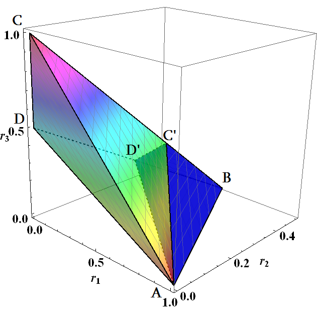
Let us assume that the spectrum of ϱX\varrho_{X} is a generic one, i.e., all eigenvalues σ⁡(ϱ):={r1,r2,r3,r4}\sigma(\varrho):=\{r_{1},r_{2},r_{3},r_{4}\} are different positive real numbers. Furthermore, in the block-diagonal representation (4) of the density matrix ϱX\varrho_{X}, the {r1,r2}\{r_{1},r_{2}\} denote the eigenvalues of the upper block and {r3,r4}\{r_{3},r_{4}\} are eigenvalues of the lower block.

The 4×44\times 4 density matrix ϱX\varrho_{X} can be diagonalized in a blockwise way,

ϱX=W⁡(diag​(r1,r2)00diag​(r3,r4))​W†,\varrho_{X}=W\left(\begin{array}[]{c|c}$\mbox{diag}$(r_{1},r_{2})&0\\ \hline\cr 0&$\mbox{diag}$(r_{3},r_{4})\\ \end{array}\right)W^{\dagger}\,, (30)

using a special unitary matrix

W=Pπ​(ei​ω​U0 0 e−i​ω​V)​Pπ,W=P_{\pi}\left(\begin{array}[]{c|c}e^{i\omega}{\displaystyle{U}}&{}^{\mbox{\Large 0 }}\\ \hline\cr{}_{\mbox{\Large 0 }}&e^{-i\omega}{\displaystyle{V}}\\ \end{array}\right)P_{\pi}, (31)

where UU and VV are 2×22\times 2 special unitary matrices diagonalizing the upper and lower sub-blocks in (4). Since a generic spectrum has been assumed, matrices UU and VV belong to the coset, S​U​(2)/U⁡(1)×S2SU(2)/U(1)\times S_{2}, where the group S2S_{2} interchanges eigenvalues inside the pairs {r1,r2}\{r_{1},r_{2}\} and {r3,r4}\{r_{3},r_{4}\}. In order to have uniqueness in (30), one can fix a certain order in the spectrum σ⁡(ϱX).\sigma(\varrho_{X}). Namely, we assume that elements of the spectrum form a partially ordered simplex, Δ¯3\underline{\Delta}_{3}, i.e.,

Δ¯3:∑i=14ri=1,0≤r2≤r1≤1,0≤r4≤r3≤1,\underline{\Delta}_{3}:\quad\sum_{i=1}^{4}r_{i}=1\,,\qquad 0\leq r_{2}\leq r_{1}\leq 1,\quad 0\leq r_{4}\leq r_{3}\leq 1\,, (32)

depicted in the Figure 1. 66 6 Note that the case of general position considered here consists of points inside the Δ¯3\underline{\Delta}_{3} and satisfies the inequalities r2<r1r_{2}<r_{1} and r4<r3.r_{4}<r_{3}\,.

Refer to caption
Figure 1: The tetrahedron A​B​C​DABCD as the image of the partially ordered simplex Δ¯3\underline{\Delta}_{3}, while the tetrahedron A​B​C′​D′ABC^{\prime}D^{\prime} inside it corresponds to a 3D simplex with the following complete order of eigenvalues: {∑i=14ri=1,1≥r1≥r2≥r3≥r4≥0}\{\ \sum_{i=1}^{4}r_{i}=1\,,\quad 1\geq r_{1}\geq r_{2}\geq r_{3}\geq r_{4}\geq 0\ \}\,.

Comparing expression (31) with (19), we convinced that the diagonalizing matrix is an element of the global group W∈GXW\in G_{{}_{X}}\, with 2×22\times 2 special unitary matrices UU and VV from the coset S​U​(2)/U⁡(1)SU(2)/U(1) parametrized by angles ϕ1,ϕ2∈[0,π],ψ1,ψ2∈[0,2​π]\phi_{1},\phi_{2}\in[0,\pi]\,,\psi_{1},\psi_{2}\in[0,2\pi]:

U=ei​ψ12​σ3​ei​ϕ12​σ2,V=ei​ψ22​σ3​ei​ϕ22​σ2.U=e^{i\displaystyle{\frac{\psi_{1}}{2}\sigma_{3}}}e^{i\displaystyle{\frac{\phi_{1}}{2}\sigma_{2}}}\,,\qquad V=e^{i\displaystyle{\frac{\psi_{2}}{2}\sigma_{3}}}e^{i\displaystyle{\frac{\phi_{2}}{2}\sigma_{2}}}\,. (33)

The 3-dimensional isotropy group HGenericH_{\mbox{Generic}} of generic orbits is

HGeneric=Pπ​(ei​ω​exp⁡γ12​σ30 0 e−i​ω​exp⁡γ22​σ3)​Pπ.H_{\mbox{Generic}}=P_{\pi}\left(\begin{array}[]{c|c}e^{i\omega}\exp{\displaystyle{\frac{\gamma_{1}}{2}\sigma_{3}}}&{}^{\mbox{\Large 0 }}\\ \hline\cr{}_{\mbox{\Large 0 }}&e^{-i\omega}\exp{\displaystyle{\frac{\gamma_{2}}{2}\sigma_{3}}}\\ \end{array}\right)P_{\pi}\,. (34)

This is in accordance with the maximal dimension of the GXG_{{}_{X}}-orbits:

dim(𝒪)Generic=dim(GX)−dimHGeneric=7−3=4.\mbox{dim}\left({\mathcal{O}}\right)_{\mbox{Generic}}=\mbox{dim}\left(G_{{}_{X}}\right)-\mbox{dim}H_{\mbox{Generic}}=7-3=4\,.

Summarising, the adjoint action of the global group GXG_{{}_{X}} determines the generic orbits, which are locally given by product of 2-spheres, S2×S2S_{2}\times S_{2}.

2.2.2 Degenerate orbits, dim​(𝒪)=2\mbox{dim}\left({\mathcal{O}}\right)=2

According to the representation (29), two types of 2D degenerate GXG_{{}_{X}}-orbits are generated by the matrices with degenerate 2×22\times 2 sub-blocks, either upper or lower blocks. In the first case the isotropy group HDegenerate H_{\mbox{\small Degenerate }} reads

HDegenerate=Pπ​(ei​ω​S​U​(2)0 0 e−i​ω​exp⁡γ22​σ3)​Pπ,H_{\mbox{\small Degenerate}}=P_{\pi}\left(\begin{array}[]{c|c}e^{i\omega}SU(2)&{}^{\mbox{\Large 0 }}\\ \hline\cr{}_{\mbox{\Large 0 }}&e^{-i\omega}\exp{\displaystyle{\frac{\gamma_{2}}{2}\sigma_{3}}}\\ \end{array}\right)P_{\pi}\,, (35)

while for the second case HDegenerate H_{\mbox{\small Degenerate }} is

H Degenerate′=Pπ​(ei​ω​exp⁡γ12​σ30 0 e−i​ω​S​U​(2)′)​Pπ.H^{\prime}_{\mbox{ \small Degenerate}}=P_{\pi}\left(\begin{array}[]{c|c}e^{i\omega}\exp{\displaystyle{\frac{\gamma_{1}}{2}\sigma_{3}}}&{}^{\mbox{\Large 0 }}\\ \hline\cr{}_{\mbox{\Large 0 }}&e^{-i\omega}SU(2)^{\prime}\\ \end{array}\right)P_{\pi}\,. (36)

In both cases, dim​HDegenerate=dim​HDegenerate′=5\mbox{dim}H_{\mbox{\small Degenerate}}=\mbox{dim}H^{\prime}_{\mbox{\small Degenerate}}=5\, and the dimension of these degenerate GXG_{{}_{X}}-orbits is

dim(𝒪)Degenerate=dim(GX)−dimHDegenerate=7−5=2.\mbox{dim}\left({\mathcal{O}}\right)_{\mbox{\small Degenerate}}=\mbox{dim}\left(G_{{}_{X}}\right)-\mbox{dim}H_{\mbox{\small Degenerate}}=7-5=2\,.

2.2.3 Degenerate orbit, dim​(𝒪)=0\mbox{dim}\left({\mathcal{O}}\right)=0

Finally, there is one point in the state space 𝔓X\mathfrak{P}_{X}\,, whose isotropy group coincides with the invariance group GX.G_{{}_{X}}\,. This point corresponds to the maximally mixed state, ϱX=14​I.\varrho_{X}=\frac{1}{4}I\,.

3 The separable states

Now we are in position to prove that every type of GXG_{{}_{X}}-orbits includes the separable states. 77 7 The density matrix ϱ\varrho\, describing the mixed state of a composed system ℋ=ℋ1⊗ℋ2,\mathcal{H}=\mathcal{H}_{1}\otimes\mathcal{H}_{2}, is separable if it allows the convex decomposition: ϱ=∑kωk​ϱ1k⊗ϱ2k,∑kωk=1,ωk>0,\varrho=\sum_{k}\omega_{k}\varrho_{1}^{k}\otimes\varrho_{2}^{k}\,,\qquad\sum_{k}\omega_{k}=1,\quad\omega_{k}>0\,, (37) where ϱ1k\varrho^{k}_{1} and ϱ2k\varrho^{k}_{2} represent the density matrices acting on the multipliers ℋ1\mathcal{H}_{1} and ℋ2\mathcal{H}_{2} correspondingly. Otherwise, it is entangled [3] .

Refer to caption
Figure 2: The absolute separable states inside the X-states tetrahedron.

3.1 Separable states on the generic GXG_{{}_{X}}-orbits

The separability of states as a function of density matrices spectrum σ⁡(ϱX)\sigma(\varrho_{X}), can be analysed using the representation (30) for the generic GXG_{{}_{X}}-orbits.

According to the Peres-Horodecki criterion [11], which is a necessary and sufficient condition for separability of 2×22\times 2 and 2×32\times 3 dimensional systems, a state ϱ\varrho is separable if its partial transposition, i.e., ϱT2=I⊗T​ϱ,\varrho^{T_{2}}=I\otimes T\varrho\,, is semi-positive as well.88 8 Here we consider the partial transposition with respect to the ordinary transposition operation TT in the second subsystem; similarly, one can use the alternative action, ϱT1=T⊗I​ϱ.\varrho^{T_{1}}=T\otimes I\varrho. Straightforward computation with ϱX\varrho_{X}\, in the form (30) shows that the semi-positivity of the partially transposed matrix ϱXT2\varrho_{X}^{T_{2}}\, requires fulfilment of the following inequalities:

(r1−r2)2​cos2⁡ϕ1+(r3−r4)2​sin2⁡ϕ2≤(r1+r2)2,\displaystyle(r_{1}-r_{2})^{2}\cos^{2}\phi_{1}+(r_{3}-r_{4})^{2}\sin^{2}\phi_{2}\leq(r_{1}+r_{2})^{2}, (38)
(r3−r4)2​cos2⁡ϕ2+(r1−r2)2​sin2⁡ϕ1≤(r3+r4)2.\displaystyle(r_{3}-r_{4})^{2}\cos^{2}\phi_{2}+(r_{1}-r_{2})^{2}\sin^{2}\phi_{1}\leq(r_{3}+r_{4})^{2}. (39)

Note that the inequalities (38) and (39) do not constraint two angles ψ1\psi_{1} and ψ2\psi_{2} in (33) that parametrize the local group K=exp⁡(i​ψ12​σ3)×exp⁡(i​ψ22​σ3).K=\exp{(i\frac{\psi_{1}}{2}\sigma_{3})}\times\exp{(i\frac{\psi_{2}}{2}\sigma_{3})}. It conforms with a general observation that the separability property is independent from the local characteristics of the composite system. This local group is the factor of the global group GX=KG′XG_{{}_{X}}=KG^{\prime}_{{}_{X}}\,, and the corresponding factor in the matrix WW diagonalising ϱX\varrho_{X}, is irrelevant for the separability of XX- states.

Analysing the inequalities (38) and (39), one can conclude:

  • i.

    There are separable states for any values of eigenvalues from the partially ordered simplex Δ¯3\underline{\Delta}_{3}. In other words, the inequalities (38) and (39) determine non-empty domain of definition for angles ϕ1\phi_{1} and ϕ2\phi_{2} in (33) for every non-degenerate spectrum σ⁡(ϱX)\sigma(\varrho_{X});

  • ii.

    There is a special family of the so-called “absolutely separable” XX-states, such that the angles ϕ1\phi_{1} and ϕ2\phi_{2} can be arbitrary one. The absolutely separable XX-states are generated by subset of the partially ordered simplex (32) defined by the inequalities

    (r1−r2)2≤4​r3​r4,\displaystyle(r_{1}-r_{2})^{2}\leq 4r_{3}r_{4}\,, (40)
    (r3−r4)2≤4​r1​r2.\displaystyle(r_{3}-r_{4})^{2}\leq 4r_{1}r_{2}\,. (41)

The Figure 2. illustrates location of the subset of the absolutely separable states inside the partially ordered simplex Δ¯3.\underline{\Delta}_{3}\,.

3.2 Separable states on the degenerate GXG_{{}_{X}}-orbits

Testing the degenerate density matrices of the form (29) by the Peres-Horodecki criterion, we reveal the following picture. The positivity requirement of partially transposed density matrix with double multiplicity of eigenvalues gives the inequalities similar to (38) and (39). However, owing to the larger isotropy group HDegenerate H_{\mbox{\small Degenerate }} of states, the new inequalities depend solely on a single coordinate of the coset GX/HDegenerate.G_{{}_{X}}/H_{\mbox{\small Degenerate}}\,. More precisely, if r1=r2,r_{1}=r_{2}\,, i.e., the degeneracy occurs in the upper sub-block, then the angle ϕ2\phi_{2} that parametrizes the matrix VV in (33) plays the role of such a coordinate. In this case, the Peres-Horodecki criterion asserts that the degenerate X−X-state is separable iff:

cos2⁡ϕ2≤4​ζ(1−ζ)2,\cos^{2}\phi_{2}\leq\frac{4\zeta}{(1-\zeta)^{2}}\,, (42)

where ζ=r4/r3<1\zeta={r_{4}}/{r_{3}}<1\,. This inequality points out the critical value ζ∗=3−2​2\zeta_{*}=3-2\sqrt{2}\,, such that for ζ≤ζ∗\zeta\leq\zeta_{*} the angle ϕ2\phi_{2} is constrained, while for the interval ζ∗<ζ<1\zeta_{*}<\zeta<1 the state is separable for an arbitrary angle ϕ2.\phi_{2}\,. The analogous results for the angle ϕ1\phi_{1} (see the matrix UU in (33)) hold true if the lower sub-block in (29) is degenerate, i.e., r3=r4.r_{3}=r_{4}\,. Therefore, in both classes of the degenerate 2D global orbits one can point out 2D family of separable degenerate states. Furthermore, among them there are the “degenerate absolutely separable” states, i.e., the degenerate global 2D orbits consisting completely from the separable states.

4 Concluding remarks

The present article is devoted to the discussion of an interplay between local and global characteristics of a pair of qubits in mixed X−X\--states. With this aim, orbits of the global unitary group GXG_{{}_{X}} action were described and classified according to the degeneracies occurring in the spectrum of density matrices. Based on this analysis, the dependence of X−X\--states separability on the spectrum has been studied. Particularly, the separable X−X\--states have been collected into the following families:

  • •

    The 4-dimensional family of separable states with the spectrum in general position;

  • •

    Two classes of 2-dimensional separable states with the double degeneracy spectrum;

  • •

    The maximally mixed state.

Finalizing notes, it is worth to comment that according to the aforementioned classification, the entangled states being complementary to the separable states, are partitioned likewise into three types. However, such classification is not complete. A further, more subtle ranging of the entangled states located on the given GXG_{{}_{X}}-orbit into subclasses is necessary. The latter subclasses are determined not by invariants of the global group GXG_{{}_{X}}, but are specified by the values of the LGXLG_{{}_{X}}-invariants. In the forthcoming publications we are planning to discuss this issue in more detail. Apart from that, following the approach elaborated in [12], [13] and [14], the generalization of the derived results for a generic case of 15-dimensional 2-qubit states will be considered.

5 Supplementary material

Here we collect a technical material useful for performing computations described in the main text. It includes the basis of the Lie algebra 𝔰​𝔲​(4)\mathfrak{su}(4), commutators of its elements and block-diagonal representation for the subalgebra αX\alpha_{X}.

∙\bulletBasis for the Lie algebra 𝔰​𝔲​(4)\mathfrak{su}(4) ∙\bullet The anti-Hermitian matrices,

{λ1,λ2,…,λ6}=i2​{σx​0,σy​0,σz​0,σ0​x,σ0​y,σ0​z}\{\lambda_{1},\lambda_{2},\dots,\lambda_{6}\}=\frac{i}{{2}}\{\sigma_{x0},\sigma_{y0},\sigma_{z0},\sigma_{0x},\sigma_{0y},\sigma_{0z}\}\,

and

{λ7,λ8,…,λ15}=i2​{σx​x,σx​y,σx​z,σy​x,σy​y,σy​z,σz​x,σz​y,σz​z},\{\lambda_{7},\lambda_{8},\dots,\lambda_{15}\}=\frac{i}{{2}}\{\sigma_{xx},\sigma_{xy},\sigma_{xz},\sigma_{yx},\sigma_{yy},\sigma_{yz},\sigma_{zx},\sigma_{zy},\sigma_{zz}\}\,,

read:

λ1=i2​‖0010000110000100‖,λ2=i2​‖00−i0000−ii0000i00‖,λ3=i2​‖1000010000−10000−1‖,\lambda_{1}=\frac{i}{2}\begin{Vmatrix}0&0&1&0\\ 0&0&0&1\\ 1&0&0&0\\ 0&1&0&0\\ \end{Vmatrix},\quad\lambda_{2}=\frac{i}{2}\begin{Vmatrix}0&0&-i&0\\ 0&0&0&-i\\ i&0&0&0\\ 0&i&0&0\\ \end{Vmatrix},\quad\lambda_{3}=\frac{i}{2}\begin{Vmatrix}1&0&0&0\\ 0&1&0&0\\ 0&0&-1&0\\ 0&0&0&-1\\ \end{Vmatrix},

λ4=i2​‖0100100000010010‖,λ5=i2​‖0−i00i000000−i00i0‖,λ6=i2​‖10000−1000010000−1‖,\lambda_{4}=\frac{i}{2}\begin{Vmatrix}0&1&0&0\\ 1&0&0&0\\ 0&0&0&1\\ 0&0&1&0\\ \end{Vmatrix},\quad\lambda_{5}=\frac{i}{2}\begin{Vmatrix}0&-i&0&0\\ i&0&0&0\\ 0&0&0&-i\\ 0&0&i&0\\ \end{Vmatrix},\quad\lambda_{6}=\frac{i}{2}\begin{Vmatrix}1&0&0&0\\ 0&-1&0&0\\ 0&0&1&0\\ 0&0&0&-1\\ \end{Vmatrix},

λ7=i2​‖0001001001001000‖,λ8=i2​‖000−i00i00−i00i000‖,λ9=i2​‖0010000−110000−100‖,\lambda_{7}=\frac{i}{2}\begin{Vmatrix}0&0&0&1\\ 0&0&1&0\\ 0&1&0&0\\ 1&0&0&0\\ \end{Vmatrix},\quad\lambda_{8}=\frac{i}{2}\begin{Vmatrix}0&0&0&-i\\ 0&0&i&0\\ 0&-i&0&0\\ i&0&0&0\\ \end{Vmatrix},\quad\lambda_{9}=\frac{i}{2}\begin{Vmatrix}0&0&1&0\\ 0&0&0&-1\\ 1&0&0&0\\ 0&-1&0&0\\ \end{Vmatrix},

λ10=i2​‖000−i00−i00i00i000‖,λ11=i2​‖000−100100100−1000‖,λ12=i2​‖00−i0000ii0000−i00‖,\lambda_{10}=\frac{i}{2}\begin{Vmatrix}0&0&0&-i\\ 0&0&-i&0\\ 0&i&0&0\\ i&0&0&0\\ \end{Vmatrix},\quad\lambda_{11}=\frac{i}{2}\begin{Vmatrix}0&0&0&-1\\ 0&0&1&0\\ 0&1&0&0\\ -1&0&0&0\\ \end{Vmatrix},\quad\lambda_{12}=\frac{i}{2}\begin{Vmatrix}0&0&-i&0\\ 0&0&0&i\\ i&0&0&0\\ 0&-i&0&0\\ \end{Vmatrix},

λ13=i2​‖01001000000−100−10‖,λ14=i2​‖0−i00i000000i00−i0‖,λ15=i2​‖10000−10000−100001‖.\lambda_{13}=\frac{i}{2}\begin{Vmatrix}0&1&0&0\\ 1&0&0&0\\ 0&0&0&-1\\ 0&0&-1&0\\ \end{Vmatrix},\quad\lambda_{14}=\frac{i}{2}\begin{Vmatrix}0&-i&0&0\\ i&0&0&0\\ 0&0&0&i\\ 0&0&-i&0\\ \end{Vmatrix},\quad\lambda_{15}=\frac{i}{2}\begin{Vmatrix}1&0&0&0\\ 0&-1&0&0\\ 0&0&-1&0\\ 0&0&0&1\\ \end{Vmatrix}.

λ1\lambda_{1} λ2\lambda_{2} λ3\lambda_{3} λ4\lambda_{4} λ5\lambda_{5} λ6\lambda_{6} λ7\lambda_{7} λ8\lambda_{8} λ9\lambda_{9} λ10\lambda_{10} λ11\lambda_{11} λ12\lambda_{12} λ13\lambda_{13} λ14\lambda_{14} λ15\lambda_{15}
λ1\lambda_{1} 0 -λ3\lambda_{3} λ2\lambda_{2} 0 0 0 0 0 0 -λ13\lambda_{13} -λ14\lambda_{14} -λ15\lambda_{15} λ10\lambda_{10} λ11\lambda_{11} λ12\lambda_{12}
λ2\lambda_{2} λ3\lambda_{3} 0 -λ1\lambda_{1} 0 0 0 λ13\lambda_{13} λ14\lambda_{14} λ15\lambda_{15} 0 0 0 -λ7\lambda_{7} -λ8\lambda_{8} −λ9-\lambda_{9}
λ3\lambda_{3} -λ2\lambda_{2} λ1\lambda_{1} 0 0 0 0 -λ10\lambda_{10} -λ11\lambda_{11} -λ12\lambda_{12} λ7\lambda_{7} λ8\lambda_{8} λ9\lambda_{9} 0 0 0
λ4\lambda_{4} 0 0 0 0 -λ6\lambda_{6} λ5\lambda_{5} 0 -λ9\lambda_{9} λ8\lambda_{8} 0 -λ12\lambda_{12} λ11\lambda_{11} 0 -λ15\lambda_{15} λ14\lambda_{14}
λ5\lambda_{5} 0 0 0 λ6\lambda_{6} 0 -λ4\lambda_{4} λ9\lambda_{9} 0 -λ7\lambda_{7} λ12\lambda_{12} 0 -λ10\lambda_{10} λ15\lambda_{15} 0 λ13\lambda_{13}
λ6\lambda_{6} 0 0 0 -λ5\lambda_{5} λ4\lambda_{4} 0 -λ8\lambda_{8} λ7\lambda_{7} 0 -λ11\lambda_{11} λ10\lambda_{10} 0 -λ14\lambda_{14} λ13\lambda_{13} 0
λ7\lambda_{7} 0 -λ13\lambda_{13} λ10\lambda_{10} 0 -λ9\lambda_{9} λ8\lambda_{8} 0 -λ6\lambda_{6} λ5\lambda_{5} -λ3\lambda_{3} 0 0 λ2\lambda_{2} 0 0
λ8\lambda_{8} 0 -λ14\lambda_{14} λ11\lambda_{11} λ9\lambda_{9} 0 -λ7\lambda_{7} λ6\lambda_{6} 0 -λ4\lambda_{4} 0 -λ3\lambda_{3} 0 0 λ2\lambda_{2} 0
λ9\lambda_{9} 0 -λ15\lambda_{15} λ12\lambda_{12} -λ8\lambda_{8} λ7\lambda_{7} 0 -λ5\lambda_{5} λ4\lambda_{4} 0 0 0 -λ3\lambda_{3} 0 0 λ2\lambda_{2}
λ10\lambda_{10} λ13\lambda_{13} 0 -λ7\lambda_{7} 0 -λ12\lambda_{12} λ11\lambda_{11} λ3\lambda_{3} 0 0 0 -λ6\lambda_{6} λ5\lambda_{5} -λ1\lambda_{1} 0 0
λ11\lambda_{11} λ14\lambda_{14} 0 -λ8\lambda_{8} λ12\lambda_{12} 0 -λ10\lambda_{10} 0 λ3\lambda_{3} 0 λ6\lambda_{6} 0 -λ4\lambda_{4} 0 -λ1\lambda_{1} 0
λ12\lambda_{12} λ15\lambda_{15} 0 -λ9\lambda_{9} -λ11\lambda_{11} λ10\lambda_{10} 0 0 0 λ3\lambda_{3} -λ5\lambda_{5} λ4\lambda_{4} 0 0 0 -λ1\lambda_{1}
λ13\lambda_{13} -λ10\lambda_{10} λ7\lambda_{7} 0 0 -λ15\lambda_{15} λ14\lambda_{14} -λ2\lambda_{2} 0 0 λ1\lambda_{1} 0 0 0 -λ6\lambda_{6} λ5\lambda_{5}
λ14\lambda_{14} -λ11\lambda_{11} λ8\lambda_{8} 0 λ15\lambda_{15} 0 -λ13\lambda_{13} 0 -λ2\lambda_{2} 0 0 λ1\lambda_{1} 0 λ6\lambda_{6} 0 -λ4\lambda_{4}
λ15\lambda_{15} -λ12\lambda_{12} λ9\lambda_{9} 0 -λ14\lambda_{14} λ13\lambda_{13} 0 0 0 -λ2\lambda_{2} 0 0 λ1\lambda_{1} -λ5\lambda_{5} λ4\lambda_{4} 0
Table 1: Commutator relations for 𝔰​𝔲​(4)\mathfrak{su(4)}.

The block-diagonal form of basis elements of subalgebra αX\alpha_{X}\, resulting under transposition PπP_{\pi}:

Pπ​λ3​Pπ=i2​(σ300−σ3),\displaystyle P_{\pi}\lambda_{3}P_{\pi}=\frac{i}{2}\left(\begin{array}[]{c|c}{\sigma_{3}}&0\\ \hline\cr 0&-\sigma_{3}\\ \end{array}\right), Pπ​λ6​Pπ=i2​(σ300σ3),\displaystyle P_{\pi}\lambda_{6}P_{\pi}=\frac{i}{2}\left(\begin{array}[]{c|c}{\sigma_{3}}&0\\ \hline\cr 0&\sigma_{3}\\ \end{array}\right),
Pπ​λ7​Pπ=i2​(σ100σ1),\displaystyle P_{\pi}\lambda_{7}P_{\pi}=\frac{i}{2}\left(\begin{array}[]{c|c}{\sigma_{1}}&0\\ \hline\cr 0&\sigma_{1}\\ \end{array}\right), Pπ​λ8​Pπ=i2​(σ200σ2),\displaystyle P_{\pi}\lambda_{8}P_{\pi}=\frac{i}{2}\left(\begin{array}[]{c|c}{\sigma_{2}}&0\\ \hline\cr 0&\sigma_{2}\\ \end{array}\right),
Pπ​λ10​Pπ=i2​(σ200−σ2),\displaystyle P_{\pi}\lambda_{10}P_{\pi}=\frac{i}{2}\left(\begin{array}[]{c|c}{\sigma_{2}}&0\\ \hline\cr 0&-\sigma_{2}\\ \end{array}\right), Pπ​λ11​Pπ=i2​(σ100−σ1),\displaystyle P_{\pi}\lambda_{11}P_{\pi}=\frac{i}{2}\left(\begin{array}[]{c|c}{\sigma_{1}}&0\\ \hline\cr 0&-\sigma_{1}\\ \end{array}\right),
Pπ​λ15​Pπ=i2​(I00−I).\displaystyle P_{\pi}\lambda_{15}P_{\pi}=\frac{i}{2}\left(\begin{array}[]{c|c}I&0\\ \hline\cr\vskip 6.0pt plus 2.0pt minus 2.0pt0&-I\\ \end{array}\right)\,.

References

  • [1] Ting Yu and J.H. Eberly. Evolution from entanglement to decoherence of bipartite mixed "X" states. Quantum Information and Computation, 7, 459-468 (2007).
  • [2] M.A. Nielsen and I.L. Chuang. Quantum Computation and Quantum Information. Cambridge University Press (2011).
  • [3] R.F. Werner. Quantum states with Einstein-Podolsky-Rosen correlations admitting a hidden-variable model. Phys. Rev. A 40(8) 4277–4281 (1989).
  • [4] M. Horodecki and P. Horodecki. Reduction criterion of separability and limits for a class of distillation protocols. Phys. Rev. A 59 4206–4216 (1999).
  • [5] S. Ishizaka and T. Hiroshima. Maximally entangled mixed states under nonlocal unitary operations in two qubits. Phys. Rev. A 62 22310 (4pp) (2000).
  • [6] F. Verstraete, K. Audenaert, T.D. Bie and B.D. Moor. Maximally entangled mixed states of two qubits. Phys. Rev. A 64 012316 (6pp) (2001).
  • [7] N.Quesada, A.Al-Qasimi and D.F.V. James, Quantum properties and dynamics of X states, Journal of Modern Optics, 59, 1322–1329 (2012).
  • [8] P. Mendonca, M. Marchiolli and D. Galetti, Entanglement universality of two-qubit X−X-states. Annals of Physics. 351, 79–103 (2014).
  • [9] A.R.P.Rau, Manipulating two-spin coherences and qubit pairs, Phys. Rev. A 61 032301 (2000).
  • [10] A.R.P.Rau, Algebraic characterization of X-states in quantum information Journal of Physics A: Mathematical and Theoretical, 42, 412002 (7pp) (2009)
  • [11] A.Peres, Separability criterion for density matrices, Phys. Rev. Lett. 77 1413-1415 (1996).
  • [12] V. Gerdt, A. Khvedelidze and Yu. Palii, On the ring of local polynomial invariants for a pair of entangled qubits, Zapiski POMI  373, 104-123 (2009).
  • [13] V. Gerdt, A. Khvedelidze and Yu. Palii, Constraints on SU(2)×\timesSU(2) invariant polynomials for entangled qubit pair, Phys. of Atomic Nucleii, Vol. 74, 893-900 (2011).
  • [14] V. Gerdt, A. Khvedelidze and Yu. Palii, On the ring of local unitary invariants for mixed X-states of two qubits, arXiv:1603.03262 [quant-ph].