ExoMol line lists XVIII. The high temperature spectrum of VO.
Abstract
An accurate line list, VOMYT, of spectroscopic transitions is presented for hot VO. The 13 lowest electronic states are considered. Curves and couplings are based on initial ab initio electronic structure calculations and then tuned using available experimental data. Dipole moment curves, used to obtain transition intensities, are computed using high levels of theory (e.g. MRCI/aug-cc-pVQZ using state-specific or minimal-state CAS for dipole moments). This line list contains over 277 million transitions between almost 640,000 energy levels. It covers the wavelengths longer than 0.29 m and includes all transitions from energy levels within the lowest nine electronic states which have energies less than 20,000 cm-1 to upper states within the lowest 13 electronic states which have energies below 50,000 cm-1. The line lists give significantly increased absorption at infrared wavelengths compared to currently available VO line lists. The full line lists is made available in electronic form via the CDS database and at www.exomol.com.
Keywords:
molecular data; opacity; astronomical data bases: miscellaneous; planets and satellites: atmospheres; stars: low-mass; stars: brown dwarfs.1 Introduction
Vanadium oxide (VO) plays an important role in astrophysical chemistry, particularly of cool stars, and is expected to also be present in brown dwarfs and hot Jupiter exoplanets. However, no comprehensive, high quality line list has been published for this molecule, limiting the potential information that can be obtained. The ExoMol project (Tennyson & Yurchenko, 2012; Tennyson & Yurchenko, 2014) aims to produce high temperature line lists of spectroscopic transitions for key molecular species likely to be significant in the analysis of the atmospheres of extrasolar planets and cool stars. The molecular data is crucial for accurate astrophysics models of the opacity, as discussed by Sharp & Burrows (2007) and Bernath (2009), and the spectroscopy of the object. However, from a chemistry perspective, vanadium is a transition metal in terms of its electronic structure and spectroscopic properties. This makes the electronic structure calculations much more difficult and gives higher uncertainties (Tennyson et al., 2016a).
VO absorption bands are generally present in cool late M class stars with effective temperature on order 2500-3000 K, mass less than 0.1 and are also expected to be observed in hot Jupiter exoplanets (Fortney et al., 2008). VO is generally present simultaneously with TiO and has similar spectroscopic and thermodynamic properties, though its abundance is about an order of magnitude less than TiO. VO tends to be more important in classifying slightly cooler (i.e. late) M dwarfs (Kirkpatrick et al., 1993; McGovern et al., 2004). VO is one of the dominant species in the spectra of young hot brown dwarfs (McGovern et al., 2004; Kirkpatrick et al., 2006; Peterson et al., 2008).

| State | Morse parameters | Properties | ||||
|---|---|---|---|---|---|---|
| /cm-1 | /Å | /cm-1 | ||||
| X | 0.000 | 1.589443 | 1.87974 | 0 | 0 | 1011.8 |
| A′ | 7293.270 | 1.622990 | 1.89529 | 0 | 0 | 946.4 |
| A | 9561.867 | 1.633621 | 1.8200∗ | 0 | 0 | 890.3 |
| B | 12655.372 | 1.640253 | 1.94733 | 0 | 0 | 912.4 |
| C | 17487.690 | 1.670620 | 1.94674 | -0.359 | 0.540 | 864.9 |
| D | 19229.786 | 1.683170 | 1.96500 | 0.060 | 0.900 | 840.9 |
| a | 5630.00∗ | 1.58200∗ | 2.0100∗ | 0 | 0 | 1041.7 |
| b | 8551.49∗ | 1.57700∗ | 2.0900∗ | 0 | 0 | 1009.0 |
| c | 9860.107 | 1.582247 | 2.07538 | 0 | 0 | 1006.1 |
| d | 10343.630 | 1.578560 | 2.16131 | 0 | 0 | 1041.7 |
| e | 15440.547 | 1.628968 | 2.0900∗ | 0 | 0 | 985.2 |
| f | 17115.919 | 1.629330 | 2.12146 | 0.226 | 0.471 | 937.2 |
| g | 18108.500 | 1.635810 | 2.17648 | 1.157 | -1.850 | 947.5 |
: Fixed based on theory or low-resolution experiment.
The A-X transition of VO, which occurs at approximately 1.05 m in the infrared, was first observed in the red giant Mira-type variable stars Mira Ceti and R Leonis by Kuiper et al. (1947), and subsequently studied more extensively by Keenan & Schroeder (1952); Spinrad & Younkin (1966); Wing et al. (1967); Spinrad & Wing (1969); Alvarez & Plez (1998) and Castelaz et al. (2000). VO has also been observed in M red-dwarf stars (Alvarez & Plez, 1998; Bernath, 2009; Rajpurohit et al., 2014). Molecular lines of VO have been detected in sunspot umbral spectra (Sriramachandran et al., 2008). Désert et al. (2008) found non-definitive evidence for VO in the atmosphere of the hot Jupiter HD209458b. Tentative detection of VO and TiO in the hot atmosphere of the hot exoplanet WASP-121b were recently reported by Evans et al. (2016).
There has been considerable recent debate (Spiegel et al., 2009; Fortney et al., 2010; Bowler et al., 2010; Madhusudhan & Seager, 2010; Huitson et al., 2012; Spiegel & Burrows, 2013; Gibson et al., 2013; Parmentier et al., 2013; Agúndez et al., 2014; Hoeijmakers et al., 2015; Schwarz et al., 2015; Haynes et al., 2015; Wakeford & Sing, 2015) about a possible temperature inversion in hot Jupiters, potentially caused by the presence of TiO and VO. Hoeijmakers et al. (2015) highlight the need for more accurate line lists to resolve this issue; though they specifically mention TiO in this paper, VO usually coexists, although it is generally thought to have a lower abundance. Line lists for TiO (Plez, 1998; Schwenke, 1998; Ryabchikova et al., 2015), despite their shortcomings, are still significantly more developed than those for VO.
Kurucz (2011) and Plez (1999) have both circulated VO line lists. Both these line lists contained only transitions in the main A-X, B-X and C-X bands (in particular, no infrared X-X transitions were included). These line lists have been used extensively in stellar and planetary models. Burrows et al. (1989) give an early study based on a simple model atmospheres incorporating TiO and VO opacities. In particular, VO is an important component of model atmospheres for M dwarfs (Allard & Hauschildt, 1995; Rajpurohit et al., 2012; Rajpurohit et al., 2014). The more complex T Tauri atmosphere models have also incorporated VO absorption bands (Herczeg & Hillenbrand, 2014).
A good VO line list is especially important in light of the new generation of proposed and planned satellites with the ability to take high quality spectra of hot Jupiters. These are required both for missions purpose-designed for studying exoplanet spectroscopy (Tinetti et al., 2012; Tennyson & Yurchenko, 2016; Tinetti et al., 2011) or more general purpose satellites such as James Webb Space Telescope (JWST) which will also have the capability to study atmospheres of hot Jupiters in 0.6– 28 m region (Beichman et al., 2014; Wakeford & Sing, 2015; Barstow et al., 2015).
VO is generally critical in modelling oxygen-rich astronomical objects with temperatures between 1500-3000 K: at lower temperatures, it condenses to more complex oxides while at higher temperatures it partially dissociates. VO may continue to be a non-negligible source of opacity and absorption up to 5000 K; therefore, we aim for a 90% complete line list up to this temperature. The resulting line list should automatically be valid for any lower temperatures.
Due to its astronomical importance in the spectroscopic analysis of M-dwarfs, the spectroscopy of diatomic VO has been well studied experimentally (Kasai, 1968; Laud & Kalsulka, 1968; Richards & Barrow, 1968a; Richards & Barrow, 1968b; Harrington & Nicholls, 1969; Cheung et al., 1981; Hocking et al., 1981; Cheung et al., 1982a; Cheung et al., 1982b; Merer et al., 1987; Merer, 1989; Huang et al., 1992; Cheung et al., 1994; Adam et al., 1995; Ram et al., 2002; Ram & Bernath, 2005; Hopkins et al., 2009). A good summary of previous experimental results is given by Miliordos & Mavridis (2007) and Hopkins et al. (2009). Generally, only the ground and first vibrational energy levels are well characterised for observed electronic states. Fortunately, transitions between quartet and doublet electronic states have been observed; this enables the relative positioning of the quartet and doublet manifold to be fixed with reasonably accuracy (limited by the fact that the absolute value of some spin-orbit terms is unknown experimentally).
The dipole moment of the ground state has been measured by Suenram et al. (1991). There is no information on the transition dipole moments of VO. However, lifetime measurements for levels in the A, B and C states were performed by Karlsson et al. (1997).
The spectroscopy of VO has also been well studied theoretically (Carlson & Moser, 1966; Wolf et al., 1977; Bauschlicher & Langhoff, 1986; Dolg et al., 1987; Bauschlicher & Maitre, 1995; Bakalbassis et al., 1996; Bridgeman & Rothery, 2000; Broclawik & Borowski, 2001; Dai et al., 2003; Pykavy & van Wullen, 2003; Mackrodt et al., 2004; Quan et al., 2006; Yao et al., 2007; Quan et al., 2008; Bande & Lüchow, 2008; Kulik & Marzari, 2010; Pradhan et al., 2011). However, the challenging nature of theoretical treatments of excited states in transition metal diatomics means that achieving quantitative accuracy is very difficult, particularly for excitation energies (Tennyson et al., 2016a). Generally, multi-reference configuration interaction (MRCI) approaches are essential.
The most detailed ab initio electronic structure study was performed by Miliordos & Mavridis (2007), who looked at the lowest nine electronic states, and also reviewed previous theoretical studies. The quality of these calculations is high, but quantitative results are only given for equilibrium values.
Another important study was performed by Hübner et al. (2015), who calculated the energetics of a much larger number of electronic states, but did not consider dipole moment or spin-orbit couplings (except for the X equilibrium dipole moment). They investigate the effect of including correlation on the internally-contracted (ic) MRCI results; however, the accuracy of the potential energy surface parameters does not show significant (if any) improvement. Their icMRCI calculations incorrectly predict the ordering of the C and D states; we find similar difficulties in reproducing the correct ordering of these states.
The goal of this paper is to produce a comprehensive line list for the main isotopologue of VO accounting for all of the lowest 13 electronic states of VO.
The structure of this article is as follows. In Section 2, the spectroscopic model for VO is developed. In Section 3, the line list for VO, named VOMYT, is constructed based on the spectroscopic model developed here and earlier (McKemmish et al., 2016). In Section 4, we compare cross-sections using the new VOMYT linelist against laboratory, observational, and previous line list spectra.
2 Constructing the Spectroscopic Model for VO
2.1 General Considerations
Astrophysically, vanadium is predominantly (99.7%) in one isotopic form, its only stable isotope, 51V.
There are three main electronic systems in VO; the A-X, B-X and C-X bands with origin (0,0) bands starting around 1.05 m (9500 cm-1), 0.79 m (12,600 cm-1) and 0.57 m (17,400 cm-1) respectively.
However, vanadium oxide, like most transition metal diatomics, has a large number of low-lying electronic states, as shown in Fig. 1. The relative energy positioning and identity of the 13 lowest electronic states (pictured) are reasonably well established by current experimental and theoretical evidence. We consider these 13 states, six quartet states and seven doublet states, in our spectroscopic model of VO; the final parameters of these states in terms of extended Morse oscillators are given in Table 1 for reference, with detailed equations later in the manuscript.
Hübner et al. (2015) considered a larger number of electronic states than we use in our model; this informs our considerations of the limitations of our 13 state electronic state spectroscopy model for VO. Specifically, we have included all nearby quartet states, but there are very many doublet states just about 20,000 cm-1 that will be involved in perturbations, spin-forbidden transitions and hot bands.
The results of Hübner et al. (2015) show that there is a significant energetic gap between these six quartet states and the next lowest quartet state (more than 12 000 cm-1). This gives confidence that there will not be additional strongly allowed electronic transitions from the ground state in the visible region.
However, there are numerous nearby higher doublet states which will certainly affect the spectroscopy of VO by perturbing the quartet states, spin-forbidden transitions and hot bands. There are not sufficient experimental data to fit these extra states and the accuracy of ab initio electronic structure calculations for these high-lying levels is not sufficient for spectroscopic purposes. It is clear that our 13 state model will not produce a full picture of the visible absorption within the doublet manifold, especially not with spectroscopic accuracy. However, the transitions involving the doublets are likely to be relatively weak, since they are either spin-forbidden or originate from excited states lying at least 5000 cm-1 above the ground state. Therefore, their absorption will contribute predominantly to the underlying continuum of VO absorption rather than to the strong signature bands; this absorption (which will particularly affect the opacity of the atmosphere) is significantly easier to model and will be less affected by perturbations in the energy levels.
We use some of the Miliordos & Mavridis (2007) results for potential energy curves as a source of data for our line list. In particular, we use their results to fit the potential energy curves of the a and b states and also use their calculation of the diagonal spin-orbit splitting of the c and e state to fix the spin-orbit splitting of the c , e and f states (the relative size of the spin-orbit coupling is known from experiment, but not their absolute values). However, Miliordos & Mavridis (2007) did not consider dipole moment (diagonal or off-diagonal), spin-orbit or electronic angular momentum coupling curves. New calculations for these properties are presented here. The spin-orbit couplings in particular can drastically affect the energy levels of the molecule.
2.2 Methodology
2.2.1 Electronic Structure Calculations
We use high level ab initio electronic structure calculations for VO by McKemmish et al. (2016), which include consideration of both static and dynamic electron correlation. In brief, the electronic structure calculations for this molecule were generally performed using Molpro (Werner et al., 2012) with the internally-contracted multi-reference configuration interaction (icMRCI) (Knowles & Werner, 1988; Werner & Knowles, 1988; Knowles & Werner, 1992) level of theory with the large aug-cc-pVQZ basis set (Dunning, 1989; Balabanov & Peterson, 2005) which incorporates diffuse functions to accurately describe the electronically excited states. The orbitals used in the icMRCI calculation were obtained using state-specific (SS) or minimal-state (MS) complete active space self-consistent field (CASSCF) calculations.
The ab initio results are shown as data points in Figs. 2,3,4,5 and 6. Note that the ab initio results often do not extend beyond about 1.8 Å. This is due to convergence difficulties associated with an ionic/covalent avoided crossing; even if calculations converged, the dipole moment obtained was often unpredictable and not smooth in this region. Changes in basis set and/or method did not significantly improve smoothness and convergence. Thus, we choose to use ab initio points only where the calculations were trusted and the curves are smooth for accurate calculation of absorption intensities below 5000 K. Smoothness is an essential feature of dipole curves if physically correct results are to be obtained (Tennyson, 2014).
The ab initio electronic structure results obtained using the above methodologies are not continuous or on a sufficiently fine grid to be used directly by a nuclear motion code to compute rovibronic energies, wavefunctions and transition intensities. Therefore, we need to interpolate and extrapolate the ab initio results to form our final spectroscopic model for VO. Due to the small number of points, simple cubic spline gave unphysical curves, particularly for the dipole moments. We thus chose to fit to physically-motivated functional forms. The choice of functional form for each property of interest is discussed as relevant.
2.2.2 Nuclear Motion Calculations
Duo is a new program (Yurchenko et al., 2016b) written by the ExoMol group that solves the nuclear motion problem for diatomics with multiple highly-coupled electronic states. The program Duo was used to produce rovibronic energy levels for VO. Input to this program were potential energy curves, spin-orbit, spin-spin and spin-rotation coupling curves and dipole moment curves. Duo allows optimisation of parameters or morphing of input curves to minimise the difference between the calculated and observed energy levels or transition frequencies that are provided.
| State | range | No | RMS | Max | |||
|---|---|---|---|---|---|---|---|
| MH from Ram et al. (2002); Ram & Bernath (2005) | |||||||
| c | 0 | 1.5 | 4.5 - 39.5 | 72 | 0.272 | 0.423 | |
| 2.5 | 4.5 - 46.5 | 86 | 0.473 | 1.757 | |||
| 1 | 1.5 | 4.5 - 39.5 | 72 | 1.078 | 3.295 | ||
| e | 0 | 2.5 | 6.5 - 39.5 | 68 | 0.109 | 0.117 | |
| 3.5 | 4.5 - 41.5 | 76 | 0.107 | 0.108 | |||
| f | 0 | 0.5 | 5.5 - 39.5 | 70 | 0.371 | 0.617 | |
| 1.5 | 4.5 - 46.5 | 86 | 0.100 | 0.227 | |||
| 1 | 0.5 | 4.5 - 39.5 | 72 | 0.493 | 1.072 | ||
| 1.5 | 4.5 - 33.5 | 60 | 0.948 | 1.007 | |||
| 2 | 0.5 | 4.5 - 39.5 | 72 | 0.467 | 0.966 | ||
| 3 | 0.5 | 6.5 - 35.5 | 59 | 0.572 | 0.976 | ||
| g | 0 | 0.5 | 0.5 - 19.5 | 40 | 0.192 | 0.376 | |
| 1.5 | 1.5 - 19.5 | 38 | 0.140 | 0.391 | |||
| 1 | 0.5 | 0.5 - 19.5 | 39 | 0.271 | 0.541 | ||
| 4 | 0.5 | 0.5 - 19.5 | 40 | 0.821 | 2.112 | ||
| MH from Merer et al. (1987) using perturbations in B-X | |||||||
| d | 2 | 0.5 | 0.5 - 39.5 | 82 | 1.079 | 8.534 | |
| 3 | 0.5 | 0.5 - 39.5 | 79 | 1.577 | 4.106 | ||
| State | range | No | RMS | Max | ||
| MH from Adam et al. (1995) | ||||||
| X | 0 | 0.5 | 0.5 - 50.5 | 101 | 0.014 | 0.040 |
| 1.5 | 1.5 - 50.5 | 100 | 0.015 | 0.041 | ||
| 1 | 0.5 | 0.5 - 50.5 | 102 | 0.017 | 0.034 | |
| 1.5 | 1.5 - 50.5 | 100 | 0.028 | 0.051 | ||
| CD from Cheung et al. (1982b) | ||||||
| A | 0 | -0.5 | 13.5 - 63.5 | 96 | 0.494 | 1.989 |
| 0.5 | 20.5 - 68.5 | 67 | 0.415 | 0.618 | ||
| 1.5 | 20.5 - 49.5 | 35 | 0.228 | 0.302 | ||
| 2.5 | 7.5 - 66.5 | 84 | 0.259 | 0.355 | ||
| CD from Cheung et al. (1994); Adam et al. (1995) | ||||||
| B | 0 | -0.5 | 5.5 - 47.5 | 80 | 0.972 | 1.402 |
| 0.5 | 4.5 - 45.5 | 68 | 1.628 | 2.380 | ||
| 1.5 | 7.5 - 40.5 | 51 | 0.505 | 1.242 | ||
| 2.5 | 7.5 - 47.5 | 76 | 0.108 | 0.393 | ||
| 1 | -0.5 | 5.5 - 24.5 | 23 | 2.421 | 3.732 | |
| 0.5 | 10.5 - 35.5 | 27 | 1.220 | 1.830 | ||
| 1.5 | 9.5 - 31.5 | 20 | 0.221 | 0.300 | ||
| 2.5 | 7.5 - 33.5 | 43 | 0.213 | 0.404 | ||
| CD from Cheung et al. (1982a) | ||||||
| C | 0 | 0.5 | 0.5 - 41.5 | 53 | 0.062 | 0.3455 |
| 1.5 | 1.5 - 38.5 | 60 | 0.260 | 1.9935 | ||
| MH from Hopkins et al. (2009) | ||||||
| C | 1 | 0.5 | 0.5 - 9.5 | 19 | 1.277 | 1.432 |
| 1.5 | 1.5 - 9.5 | 18 | 1.425 | 1.570 | ||
| 2 | 0.5 | 0.5 - 9.5 | 20 | 3.286 | 3.43 | |
| 1.5 | 1.5 - 9.5 | 18 | 2.937 | 2.964 | ||
| 3 | 0.5 | 0.5 - 9.5 | 10 | 1.655 | 1.857 | |
| 1.5 | 1.5 - 9.5 | 9 | 1.872 | 2.040 | ||
| 4 | 0.5 | 0.5 - 9.5 | 20 | 1.705 | 1.906 | |
| 1.5 | 1.5 - 9.5 | 18 | 1.873 | 2.093 | ||
| 5 | 0.5 | 0.5 - 9.5 | 20 | 2.140 | 2.796 | |
| 1.5 | 1.5 - 9.5 | 18 | 2.007 | 2.480 | ||
| 6 | 0.5 | 0.5 - 9.5 | 18 | 0.949 | 1.466 | |
| 1.5 | 1.5 - 9.5 | 18 | 0.998 | 1.203 | ||
| State | range | No | RMS | Max | ||
|---|---|---|---|---|---|---|
| CD from A fit and D-A in Merer et al. (1987) | ||||||
| D | 0 | 0.5 | 6.5 - 23.5 | 10 | 2.325 | 2.446 |
| 1.5 | 8.5 - 25.5 | 34 | 0.186 | 0.468 | ||
| 2.5 | 14.5 - 14.5 | 2 | 0.460 | 0.469 | ||
| 3.5 | 6.5 - 24.5 | 32 | 0.441 | 0.484 | ||
| CD from D fit and D-A′ in Merer et al. (1987) | ||||||
| A′ | 0 | 1.5 | 5.5 - 6.5 | 2 | 17.448 | 17.506 |
| 2.5 | 8.5 - 28.5 | 8 | 8.435 | 10.269 | ||
| 3.5 | 8.5 - 47.5 | 21 | 1.498 | 2.588 | ||
| 4.5 | 13.5 - 42.5 | 7 | 4.072 | 5.710 | ||
| 1 | 2.5 | 15.5 - 18.5 | 2 | 2.023 | 4.246 | |
| 3.5 | 13.5 - 46.5 | 30 | 1.108 | 2.272 | ||
| 4.5 | 19.5 - 31.5 | 7 | 3.641 | 5.106 | ||
| 2 | 3.5 | 15.5 - 39.5 | 21 | 0.662 | 1.324 | |
| 4.5 | 19.5 - 39.5 | 20 | 1.583 | 2.746 | ||
| Transition | range | range | No | RMS | Max | ||||
|---|---|---|---|---|---|---|---|---|---|
| A -X | 0 | -0.5 | 17.5 - 49.5 | 0 | 0.5 | 16.5 - 50.5 | 42 | 0.376 | 0.633 |
| 0.5 | 30.5 - 63.5 | 1.5 | 31.5 - 63.5 | 25 | 0.510 | 0.662 | |||
| 1.5 | 17.5 - 49.5 | 1.5 | 16.5 - 49.5 | 20 | 0.237 | 0.315 | |||
| 2.5 | 28.5 - 62.5 | 0.5 | 29.5 - 63.5 | 27 | 0.183 | 0.414 | |||
| 2.5 | 8.5 - 65.5 | 1.5 | 8.5 - 66.5 | 46 | 0.076 | 0.260 | |||
| -0.5 | 19.5 - 49.5 | 1 | 0.5 | 18.5 - 50.5 | 35 | 0.393 | 0.593 | ||
| -0.5 | 30.5 - 63.5 | 1.5 | 31.5 - 63.5 | 15 | 0.396 | 0.686 | |||
| 1.5 | 17.5 - 49.5 | 1.5 | 16.5 - 49.5 | 20 | 0.228 | 0.318 | |||
| 2.5 | 8.5 - 33.5 | 1.5 | 8.5 - 32.5 | 24 | 0.086 | 0.232 | |||
| B -X | 0 | -0.5 | 6.5 - 46.5 | 0 | 0.5 | 7.5 - 46.5 | 38 | 0.932 | 1.290 |
| 0.5 | 4.5 - 46.5 | 1.5 | 4.5 - 46.5 | 96 | 0.970 | 1.412 | |||
| 1.5 | 7.5 - 37.5 | 0.5 | 6.5 - 37.5 | 36 | 0.517 | 0.959 | |||
| 1.5 | 6.5 - 40.5 | 1.5 | 5.5 - 39.5 | 47 | 0.463 | 1.227 | |||
| 2.5 | 8.5 - 36.5 | 0.5 | 7.5 - 35.5 | 15 | 0.077 | 0.102 | |||
| 2.5 | 6.5 - 47.5 | 1.5 | 5.5 - 47.5 | 105 | 0.107 | 0.226 | |||
| 1 | -0.5 | 5.5 - 23.5 | 0 | 1.5 | 5.5 - 23.5 | 21 | 2.429 | 3.442 | |
| 1.5 | 8.5 - 28.5 | 1.5 | 7.5 - 29.5 | 22 | 0.212 | 0.293 | |||
| 2.5 | 6.5 - 33.5 | 1.5 | 5.5 - 33.5 | 60 | 0.220 | 0.429 | |||
| C -X | 0 | 0.5 | 4.5 - 40.5 | 0 | 0.5 | 4.5 - 40.5 | 44 | 0.041 | 0.138 |
| 1.5 | 2.5 - 38.5 | 1.5 | 2.5 - 38.5 | 79 | 0.042 | 0.103 |
| Transition | range | range | No | RMS | Max | ||||
|---|---|---|---|---|---|---|---|---|---|
| D -A | 0 | 0.5 | 6.5 - 23.5 | 0 | -0.5 | 6.5 - 24.5 | 10 | 0.204 | 0.421 |
| 1.5 | 8.5 - 24.5 | 0.5 | 7.5 - 25.5 | 47 | 0.309 | 0.682 | |||
| 2.5 | 14.5 - 14.5 | 1.5 | 13.5 - 14.5 | 3 | 0.604 | 0.643 | |||
| 3.5 | 6.5 - 24.5 | 2.5 | 5.5 - 23.5 | 41 | 0.442 | 0.500 | |||
| D -A′ | 0 | 0.5 | 2.5 - 7.5 | 0 | 1.5 | 3.5 - 6.5 | 6 | 11.201 | 11.266 |
| 1.5 | 7.5 - 28.5 | 2.5 | 8.5 - 28.5 | 13 | 3.069 | 4.039 | |||
| 2.5 | 7.5 - 48.5 | 3.5 | 8.5 - 47.5 | 49 | 0.922 | 1.877 | |||
| 3.5 | 12.5 - 43.5 | 4.5 | 13.5 - 42.5 | 14 | 1.413 | 2.194 | |||
| 1.5 | 14.5 - 18.5 | 1 | 2.5 | 15.5 - 18.5 | 4 | 0.588 | 0.636 | ||
| 2.5 | 12.5 - 47.5 | 3.5 | 13.5 - 46.5 | 75 | 0.756 | 1.190 | |||
| 3.5 | 18.5 - 31.5 | 4.5 | 19.5 - 31.5 | 14 | 7.292 | 8.219 | |||
| 1 | 1.5 | 11.5 - 19.5 | 0 | 2.5 | 12.5 - 19.5 | 3 | 3.632 | 4.092 | |
| 2.5 | 13.5 - 39.5 | 2 | 3.5 | 14.5 - 39.5 | 53 | 0.785 | 1.018 | ||
| 3.5 | 18.5 - 39.5 | 4.5 | 19.5 - 39.5 | 47 | 4.818 | 6.060 |
2.2.3 Collation and Selection of Experimental Data
The use of experimental data is imperative to ExoMol’s methodology, particularly for molecules like VO where current ab initio electronic structure methods do not deliver sufficient accuracy as discussed by McKemmish et al. (2016) and Tennyson et al. (2016a) in detail. An important component of the line list generation is thus the collation and selection of a set of empirical energies and frequencies. The spectroscopic model has been refined to minimize the root mean squared deviation of the Duo predicted (calculated) energy levels and/or frequencies against the empirical (observed) values.
Tables 2, 3, 4, 5 and 6 detail the major sources of experimental data used to construct the Duo spectroscopic model of VO.
Experimental transitions involving the doublet c , e , f and g states have been measured and used to construct model Hamiltonians fits for each spin-vibronic band. Some spin-forbidden doublet-to-quartet transitions have recently been observed (g -X ) by Hopkins et al. (2009) which are extremely useful in fixing the relative positions of the doublet and quartet states. However, these observed transitions do not quite provide sufficient information to determine the energy of all spin rovibronic bands relative to the zero of the X state. Specifically, there is a spectroscopic network connecting the {c 5/2, e 7/2, f 3/2 and g 3/2} states from the experiments reported by Merer et al. (1987), Ram et al. (2002) and Ram & Bernath (2005) via the observed g 3/2-X transition. This network can be connected to the ground state of VO. However, the spectroscopic network comprising {c 3/2, e 5/2, f 1/2} is not connected to g 1/2 and therefore also not to the X state and the absolute energy scale of VO. Nevertheless, the relative spin-orbit coupling matrix elements of the c , e and f are known from experiment, as detailed in Table 8. We can thus use a single magic number (Furtenbacher et al., 2007) to connect the two spectroscopic networks. Based on ab initio electronic structure predictions by Miliordos & Mavridis (2007) and our own calculations, we choose this magic number by setting the spin-orbit coupling constant of the c state to 180 cm-1. Using this magic number and the spin-forbidden transitions, we can then set the absolute for each doublet state. The model Hamiltonians given in the original experimental papers can then be used to produce empirical energies using PGopher (Western, 2016). The range of the energy levels we used was informed by the experimental data available in the original paper. The use of experimental energies from model Hamiltonian fits was judged sufficient for doublet states for two reasons: (1) the intensity of their transitions do not contribute significantly to the final absorption spectra and (2) the spin and rotational structure of doublet spectra are easier to fit (and hence more reliable) than for quartet spectra. Furthermore, manual checks of the reported frequencies against our calculated PGopher empirical energy levels showed good agreement. Table 2 details all the spin-vibronic bands of doublet states which we include in to refine the spectroscopic model. Note that we also include data on some d bands; these were not directly measured but inferred from perturbations to the B-X transitions.
For quartet states, we found some significant discrepancies between the calculated PGopher empirical energy levels and the frequencies reported in the original experimental manuscripts, particularly for the A-X transition. The origin of the differences could be typographic errors or different definitions of model Hamiltonian constants. Instead of retracing this error, we decided to use the frequencies directly as our source of experimental data. Assuming the model Hamiltonian representation of the X state (reasonable given the significant amount of data involving this state, and the consistency with latter combination differences), we produced empirical energy levels for the X state using PGopher. Based on these lower state energies, we could derive the upper state energies (e.g. the A , B and C state energies) from the experimental frequencies based on the assignments given in the original paper. The ‘combination differences’ method was used in which an upper state energy was only trusted if two or more transitions gave the same energy for a particular upper state (within a threshold; here selected to be the relatively loose 0.2 cm-1). This process yielded a set of A , B and C upper state rovibronic energy levels and their associated quantum numbers. We also had a set of A-X, B-X and C-X frequencies for which the assigned quantum numbers had been verified through combination differences. Finally, Hopkins et al. (2009) measured some vibrational excited and overtone bands of the C-X transition. We use the model Hamiltonian fits and PGopher to produce empirical energy levels of these vibrationally excited C states. Table 3 details all the X , A , B and C spin-vibronic band energies which we include in the model refinement, while Table 5 details the transitions used.
The D and A′ energy levels are obtained indirectly using the A-X, D-A, D-A′ transitions. Given the difficulties in the model Hamiltonian parameters for the A state, we decided to not use the energy levels from D and A′ model Hamiltonian parameters. Instead, we used the Duo energy levels for the A state in combination with D-A transition frequencies to obtain combination differences for the D state. After fitting to the D state in Duo, we used the Duo D state energies and the D-A′ transition frequencies to obtain combination differences for the A′ state. We refine our model to both these D and A′ combination difference energies (see Table 4) and the D-A and D-A′ frequencies (see Table 6) that produced these combination differences.
For such a complex molecule, the refinement of the theoretical model to experimental data needs to be performed iteratively.
In the first step, we used the independent electronic state approximation to find potential energy curves and diagonal spin-orbit couplings for each of the electronic states assuming that there was no interaction between electronic states. The independent state approximation was then relaxed through the inclusion of off-diagonal spin-orbit coupling and electronic angular momentum coupling terms.
The final parameters are detailed in the next section and provided in Duo input format as part of the supplementary information for this article.
| State | Method/ Source | Property | Value |
|---|---|---|---|
| Experimental data | |||
| A | Tentative assignment1 | 884 cm-1 | |
| a | Low-res. Photoelectron2 | 5630 cm-1 | |
| Ab initio data3 | |||
| a | C-icMRCI+DKH2+Q/BP | 1.582 Å | |
| 1020 cm-1 | |||
| b | C-icMRCI+DKH2+Q/BP | 8849 cm-1 | |
| 1.577 Å | |||
| icMRCI+Q/B | 1025 cm-1 | ||
| e | icMRCI+Q/B | 934 cm-1 | |
| c | icMRCI/BP | SO | 180 cm-1 |
2.3 Results
2.3.1 Potential Energy Curves
The potential energy curves of the 13 electronic states is the most important component of the VO spectroscopic model. It controls the main rovibronic energy structure (i.e. the gaps between electronic states, the vibrational spacing and the rotational constants).
The high dissociation energy of VO means that the Morse oscillator is a good representation of the potential energy curves (PEC) for the low-lying electronic states of VO in the region of interest. This observation combined with the lack of reliable ab initio electronic structure results at long bond lengths/ higher energies meant that we did not use ab initio PECs as input into Duo. Instead we directly used the extended Morse oscillator (EMO) potential (Lee et al., 1999)
| (1) |
We started by setting the and parameters to zero, reducing the EMO to a simple Morse oscillator. We fixed the dissociation energy of the X state to 52290 cm-1 based on experiment (Balducci et al., 1983); + for all other states was also fixed to this value, since all electronic states considered dissociate to the same atomic limit. Then the empirical excitation energies, harmonic frequencies and equilibrium bond lengths were used to find initial parameters. Note that in Duo default inverse length units, Å-1, the Morse oscillator parameter where if and are in cm-1 and the reduced mass is in Dalton then . Where the term energies, harmonic frequencies and/or equilibrium bond lengths were unknown, we used ab initio electronic structure calculations data from Miliordos & Mavridis (2007) as summarised in Table 7.
The , and parameters were then modified to reproduce the energy levels and frequencies in Tables 2, 3, 5, 4, 6. For the C , D , f and g states, there was sufficient experimental data available to also optimise and . The final parameters for the PEC of the spectroscopic model of VO are given in Table 1.
| Ab Initio | Extrapolation Parameters | Duo Fit | Exp | |||||||
| Fit? | ||||||||||
| A′ | 256.26 | OF | 181.8 | 0.66 | 1∗ | 255.16 | 179.36 | 251.71 | 256.2 | |
| A | 68.99 | GF | 140.3 | -0.97 | 1.31 | 69.06 | 106.98 | 52.64 | 52.8 | |
| B | 90.63 | GF | 63.5 | 1.21 | 2.11 | 90.63 | 67.98 | 97.02 | 96.9 | |
| D | 169.81 | WC | 155.2 | 0.15 | 1∗ | 169.28 | 131.70 | 143.68 | 143.5 | |
| b | 0.71 | GF | 2.1 | -1.05 | 1∗ | 0.72 | ||||
| c | 188.02 | TPS | 187.7 | 0∗ | N/A | 187.73 | 179.81 | 179.81 | # | |
| e | 176.54 | WC | 140.5 | 0.41 | 1∗ | 175.62 | 148.28 | 185.34 | # + 6.1 | |
| f | Exp | 126.4 | 0∗ | N/A | 126.41 | 126.41 | 126.41 | # 54.4 | ||
| g | 61.96 | OF | 76.8 | -1.47 | 4∗ | 60.76 | 72.82 | 57.65 | 59.8 | |
∗ Parameter constrained. # Experiment constrains the ratio between these three spin-orbit matrix elements, but not their exact value. Based on the theory calculations of Miliordos & Mavridis (2007), we constrained cm-1.


| Ab Initio | Extrapolation Parameters | |||||||
| Fit? | Matrix Element | |||||||
| X-A | 65.98 | GF | 91.6 | -0.45 | 1∗ | 65.82 | ||
| X-B | 7.89 | OF | 86.1 | -1.43 | 1∗ | 8.70 | ||
| A′-D | 43.03 | OF | 41.5 | 1.31 | 7.70 | 43.06 | ||
| A-B | 2.70 | TPS | 2.2 | 0∗ | N/A | 2.22 | ||
| A-C | 6.39 | WC | 54.6 | -1.41 | 1∗ | 6.29 | ||
| A-D | 45.37 | WC | 20.5 | 1.90 | 1∗ | 44.89 | ||
| B-C | 41.70r=1.57 | TPS | 41.8 | 0.0 | N/A | 41.83 | ||
| B-D | 4.73 | OF | 39.4 | -1.38 | 1∗ | 5.32 | ||
| X-d | 265.95 | OF | 277.6 | -0.29 | 4∗ | 265.19 | ||
| X-f | 57.79 | OF | 60.6 | -0.29 | 4∗ | 57.88 | ||
| X-g | 78.27 | WC | 89.4 | -0.20 | 1∗ | 78.40 | ||
| A′-b | 82.28 | TPS | 82.0 | 0∗ | N/A | 81.96 | ||
| A′-c | 32.39 | GF | 140.6 | -1.20 | 1∗ | 32.35 | ||
| A′-e | 122.27 | WC | 80.1 | 0.83 | 1∗ | 121.75 | ||
| A-a | 48.76 | TPS | 48.5 | 0∗ | N/A | 48.48 | ||
| A-c | 8.89 | TPS | 8.6 | 0∗ | N/A | 8.63 | ||
| A-d | 62.02 | WC | 10.6 | 7.58 | 1∗ | 60.92 | ||
| A-f | 22.33 | TPS | 25.0 | 0∗ | N/A | 25.01 | ||
| A-g | 216.32 | WC | 171.5 | 0.40 | 1∗ | 215.13 | ||
| B-a | 16.37 | GF | 48.8 | -2.72 | 3.05 | 16.45 | ||
| B-c | 8.89 | TPS | 8.6 | 0∗ | N/A | 8.63 | ||
| B-d | 6.96 | GF | 13.8 | -1.80 | 2.79 | 6.98 | ||
| B-f | 12.14r=1.65 | WC | -20.8 | -2.49 | 1∗ | 11.82 | ||
| B-g | 12.86r=1.47 | WC | 25.9 | -0.74 | 1∗ | 13.85 | ||
| C-d | 18.85 | GF | 77.2 | -1.19 | 1∗ | 19.22 | ||
| C-f | 6.40r=1.61 | OF | 17.4 | -4.11 | 4∗ | 6.20 | ||
| C-g | Not calculated | 0∗ | 0∗ | N/A | ||||
| D-c | 14.53r=1.58 | OF | 102.3 | -1.34 | 1∗ | 15.78 | ||
| D-e | 32.21 | WC | 35.2 | -0.13 | 1∗ | 32.26 | ||
| D-f | 36.49 | TPS | 36.0 | 0∗ | N/A | 36.04 | ||
| D-g | 34.53 | GF | 23.1 | 3.62 | 4.32 | 34.41 | ||
| a-d | 192.33 | OF | 200.7 | -0.28 | 4∗ | 191.80 | ||
| a-f | 78.62 | GF | 94.9 | -0.27 | 1∗ | 78.64 | ||
| a-g | 68.86 | OF | 94.9 | -0.27 | 1∗ | 68.55 | ||
| b-e | 69.01 | TPS | 68.8 | 0∗ | N/A | 68.47 | ||
| c-e | 12.35 | OF | 76.4 | -1.32 | 1∗ | 13.21 | ||
| c-f | 19.21 | OF | 60.3 | -1.09 | 1∗ | 19.14 | ||
| c-g | 34.66r=1.61 | OF | 134.4 | -1.20 | 1∗ | 33.36 | ||
| d-f | 53.52 | WC | 21.7 | 2.30 | 1∗ | 52.99 | ||
| d-g | 2.97 | TPS | 2.7 | 0∗ | N/A | 2.67 | ||
| f-g | 150.95r=1.56 | GF | 111.86 | 0.54 | 1∗ | 150.19 | ||
∗ Parameter constrained.


2.3.2 Spin-Orbit Coupling Curves
The spin-orbit coupling constants have two main effects in the spectroscopy of VO. First, diagonal coupling terms split the energies of the different spin components of the quartet or doublet electronic state with non-zero electronic angular momentum . This significantly increases the complexity of the spectra of molecules with high spin states such as VO compared to more common main-group chemical molecules like . Second, off-diagonal spin-orbit coupling causes mixing between different electronic states of both the same and different spins. This mixing gives intensity to spin- and symmetry-forbidden transitions, significantly increasing the complexity of the final spectra, though most of these new lines are quite weak compared to the allowed bands. In fact, the inclusion of off-diagonal spin-orbit coupling in our spectroscopic model is the major contributor (with Lx coupling playing a smaller but important role) to the very large number of transitions in the ExoMol VOMYT line list compared to the earlier Plez and Kurucz line lists.
We fit the absolute value of the ab initio data to the form:
| (2) |
where is the bond distance, are parameters, and is used to ensure sufficiently fast convergence to the atomic value . For many coupling elements, the data is insufficient to provide a strong constraint on the variable parameters and consequently there can be a lot of variance in the fitted value of . Thus, different spin-orbit curves should be compared by the equilibrium value not the asymptotic value because the equilibrium value is generally interpolated not extrapolated.
To fit experimental data, and introduce the correct sign and phase information, we included a further multiplicative value, , i.e.
| (3) |
may be complex.
The specifications for the diagonal spin-orbit coupling curves are tabulated in Table 8, while the ab initio data points and fits are plotted for quartets and doublets in Fig. 2. The specifications for the off-diagonal spin-orbit coupling curves are tabulated in Table 9, while the ab initio data points and fits are plotted in Fig. 3. One result worth commenting about is the f and g spin-orbit coupling. Experimentally, there is little evidence of coupling between the f and g states; the fact that our ab initio electronic structure calculations give a large spin-orbit coupling constant is indicative of mixing between the f and g in the ab initio calculation (since the two states share the same spin and symmetry). We choose to include this spin-orbit coupling because it should improve dipole moment matrix elements involving the f and g states.
| With D-g SO | No D-g SO | ||||||
|---|---|---|---|---|---|---|---|
| State | range | No. | RMS/cm-1 | Max/cm-1 | RMS/cm-1 | Max/cm-1 | |
| D | 0.5 | 6.5 - 23.5 | 10 | 15.95 | 18.00 | 1.11 | 2.02 |
| 1.5 | 8.5 - 25.5 | 35 | 7.43 | 10.24 | 0.65 | 1.33 | |
| 2.5 | 14.5 - 14.5 | 2 | 0.42 | 0.42 | 0.35 | 0.36 | |
| 3.5 | 6.5 - 24.5 | 32 | 0.56 | 1.00 | 0.56 | 1.00 | |
In most cases, ab initio spin-orbit coupling constants were found to be generally reliable; in particular, our diagonal spin-orbit constants were usually very accurate. However, calculations involving states A , B , f or g showed much larger errors. In particular the f , g state were often not in the right order with respect to each other and the h state. These errors partially arise due to significant mixing between nearby states of the same spin and symmetry: the A and B state share the same spin and symmetry and are only approximately 3000 cm-1 apart, while the f and g states are even closer at approximately 1000 cm-1 apart and within 3000 cm-1 of a third state of the same spin and symmetry, h . A specific example of the errors this caused in the final line list can be seen in the energy levels of the D state given in Table 10 with and without the inclusion of the D-g spin-orbit coupling constants (with other parameters optimised). The inclusion of the D -g spin-orbit coupling constant significantly deteriorates the quality with which the Duo model reproduces the D state combination differences. Given these ab initio difficulties combined with the fact there are other very closely lying states that are not considered in our model, we choose not to include many diagonal spin-orbit coupling elements involving the f and g states. The only exceptions are the f -g and A -g spin-orbit coupling elements.
| Ab Initio | Extrapolation Parameters | ||||||
| Fit? | |||||||
| X-A | 1.320 | GF | 1.5∗ | 1.34 | 4.34 | 1.321 | |
| X-B | 0.016 | GF | 0.5∗ | -0.76 | 1∗ | 0.020 | |
| A′-D | 0.512 | OF | 1∗ | -0.78 | 1∗ | 0.510 | |
| A-C | 1.063 | TPS | 1∗ | 0.08 | 1∗ | 1.049 | |
| A-D | 0.549 | TPS | 0.5∗ | -0.72 | 4∗ | 0.557 | |
| B-C | 0.128 | OF | 0.5∗ | -0.86 | 1.76 | 0.121 | |
| B-D | 0.131r=1.61 | GF | 0.5∗ | -1.44 | 2.86 | 0.117 | |
| a-f | 0.301 | OF | 1∗ | -1.54 | 1.70 | 0.300 | |
| a-g | 0.072 | TPS | 0∗ | 0.10 | 1∗ | 0.064 | |
| b-e | 0.016 | TPS | 0∗ | 0.03 | 1∗ | 0.016 | |
| c-e | 0.217r=1.58 | GF | 1∗ | -1.46 | 1.36 | 0.223 | |
| c-f | 0.301 | GF | 1∗ | -1.54 | 1.70 | 0.300 | |
| c-g | 0.175r=1.61 | OF | 1∗ | -1.32 | 1∗ | 0.172 | |
| d-f | 0.049 | TPS | 0∗ | 0.07 | 1∗ | 0.041 | |
| d-g | 1.538 | GF | 2∗ | -1.12 | 1.93 | 1.542 | |
∗ Parameter constrained.


2.3.3 Lx coupling
The Lx coupling is the electronic angular momentum coupling between electronic states. It acts in a similar way to the spin-orbit coupling to give rise to mixing of electronic states and the weak occurence of some previously forbidden spectral lines. However, Lx coupling has a much smaller effect because diagonal elements and coupling between electronic states of different spins is strictly zero.
We fit the absolute of the ab initio data to the form:
| (4) |
where to ensure sufficiently fast convergence to the atomic limiting value . When the data supports a particular logical rational value of (e.g. 0 or 1), this value is fixed.
The input to the Duo program was given by
| (5) |
The parameter was used to provide the correct sign and phase information appropriate to Duo and may be complex; getting the sign correct from Molpro output to Duo output is non-trivial (Patrascu et al., 2014). It could also be used in fitting; however, this was not done in the case of VO.
The ab initio points and the fit are shown graphically in Fig. 4. The specifications of the ab initio data, the fit and the Duo input are given in Table 11.
It is difficult to judge the accuracy of the theoretical electronic angular momentum terms. For VO, inclusion of all of these terms did not adversely affect the fit; therefore we included non-zero terms involving the lowest 13 electronic states. Note, however, that there are a significant number of electronic states just above 20,000 cm-1 that will couple to lower states, in particular the f , g , C and D states.
| State | Fitted∗ | Exp | |
|---|---|---|---|
| X | 0.0529 | 2.0300 | |
| 0.0191 | 0.0225 | ||
| A′ | -0.6030 | ||
| 0.4400 | |||
| A | 1.0410 | 1.8670 | |
| 0.0065 | 0.0038 | ||
| B | 2.5869 | 2.6579 | |
| 0.0452 | 0.0336 | ||
| C | 0.8037 | 0.7469 | |
| -0.0155 | -0.0184 | ||
| D | 0.2625 | ||
| 0.0160 | |||
| c | 0.2340 | ||
| e | -0.0864 | ||
| f | -0.1520 | ||
| g | 1.2500 |
∗ Note that Duo actually takes as input ; values are tabulated to match experiment.
2.3.4 Spin-Spin and Spin-Rotational Constants
Traditionally, the model Hamiltonians used to fit observed data often included empirical spin-spin and spin-rotation elements. These matrix elements always involve only one electronic state. They quantify how the energy of a particular energy level depends on its spin state and the rotational levels. The effect of the spin-spin coupling is much smaller than the spin-orbit coupling, but can be important for high accuracy and when there is no orbital angular momentum (and therefore no diagonal spin-orbit coupling). The spin-rotation element is again generally a small effect needed only for very high accuracy reproduction of energy levels. The spin-spin and spin-rotation elements are physical components of the total spin-rovibronic Hamltonian (Tennyson et al., 2016a). Though it is theoretically possible to calculate these terms, this is not routinely done due to computational difficulty and also because these terms are usually also empirical corrections for interactions that have been neglected in the model.
Since these are empirical terms that asympotically go to zero, we decided to use the Surkus-polynomial expansion (Šurkus et al., 1984) formula for their matrix elements:
| (6) |
where Å, and is an adjustable parameter, given by for spin-spin constants and for spin-rotation constants. Note that the form of this expression is such that the matrix elements go to zero asymptotically. The value of the included spin-spin and spin-rotation terms are specified in Table 12, and compared against previously empirical (equilibrium) values where available. In many cases, the previous empirical values agree quite well to our values. The major difference is the spin-spin constant of the X state which is only about 2.5% of the experimental value. This reduction occurs because the spin-orbit couplings (particularly between the X-d states) produce the same type of perturbation to the X state energy levels as the spin-spin coupling constant. However, the effect on other energy levels will be different, and some spin-forbidden transitions may be given intensity through this mechanism. The importance of the X-d spin-orbit coupling explaining the splitting of the X state energy levels could not be predicted by experiment, as the X and d states are more than 10,000 cm-1 apart; it is only the very large magnitude (approximately 250 cm-1) of the spin-orbit coupling constant that makes this element important. This example illustrates that the spin-spin coupling constants are sometimes used as empirical corrections rather than a fundamental characteristic. Proper accounting for important spin-orbit coupling can provide a more accurate picture of the molecule’s spectroscopy. unfortunately, for higher lying electronic states, this is currently impossible for transition metal diatomics with the high density of electronic states and the quality of modern ab initio calculations (Tennyson et al., 2016a).


| State | Ab Initio | Extrapolation Parameters | Fit Characteristics | ||||||||
|---|---|---|---|---|---|---|---|---|---|---|---|
| Range (Å) | for | ||||||||||
| X | 1.15 - 1.99 | -2.943 | 3∗ | -13.440 | 3.830 | 0.000 | -8.812 | -2.958 | -6.656 | -5.975 | 2.413 |
| A′ | 1.24-1.91 | -3.281 | 3.493 | -2.801 | 2.503 | 13.519 | -28.013 | -3.279 | -5.401 | -4.623 | 2.370 |
| A | 1.20-1.80 | -3.263 | 2.617 | -4.356 | 2.320 | 11.368 | -23.962 | -3.253 | -5.302 | -4.967 | 2.408 |
| B | 1.40-1.65 | -5.996 | 3∗ | -0.846 | 6.123 | 18.798 | -42.106 | -5.993 | -8.209 | -10.171 | 3.237 |
| a | 1.25 - 1.92 | -1.319 | 0.859 | -5.042 | 0.630 | 6.478 | -13.689 | -1.311 | -4.008 | -2.453 | 2.259 |
| b | 1.41-1.80 | -2.359 | 1.876 | -9.668 | 2.468 | 3.058 | -11.127 | -2.361 | -5.673 | -4.623 | 2.37 |
| c | 1.41-1.61 | 0.244 | Fit to | 0.252 | -1.878 | ||||||
| d | 1.41-1.80 | -2.318 | 1.368 | -2.849 | 2.819 | 4.671 | -14.822 | -2.315 | -5.520 | -4.590 | 2.479 |
| e | 1.41-1.76 | -2.814 | 1.039 | -4.333 | 0.719 | 12.126 | -21.054 | -2.857 | -4.189 | -3.782 | 2.155 |
∗: constrained to ensure reasonable fit.
| Ab Initio | Extrapolation Parameters | |||
|---|---|---|---|---|
| X-A | 0.19 | 1.306 | 2.122 | 0.192 |
| X-B | 0.613 | 6.451 | 3.054 | 0.616 |
| X-C | 1.149 | 7.627 | 2.079 | 1.145 |
| A′-D | 0.106 | 1.195 | 3∗ | 0.112 |
| A-B | 0.067 | Inbuilt Duo interpolation | ||
| A-C | 0.186 | 1.294 | 2.172 | 0.186 |
| A-D | 0.11 | 0.452 | 1∗ | 0.11 |
| B-C | 0.06 | 0.480 | 2.428 | 0.061 |
| B-D | 0.018r=1.61 | 1.657 | 7.596 | 0.019 |
| a-f | 0.025 | 1.454 | 6.75 | 0.025 |
| a-g | 0.011 | 0.033 | 0.397 | 0.011 |
| b-e | 0.061 | 0.346 | 1.733 | 0.061 |
| c-e | 0.275r=1.58 | 2.384 | 2.68 | 0.27 |
| c-f | 0.276 | 2.539 | 2.772 | 0.276 |
| c-g | 0.071r=1.61 | 1.408 | 4.299 | 0.076 |
| d-f | 0.067 | 0.407 | 1.848 | 0.068 |
| d-g | 0.052 | 1.045 | 4.371 | 0.054 |
∗ Parameter constrained.


2.3.5 Diagonal Dipole Moment Curves.
All diagonal dipole moment curves use icMRCI/aug-cc-pVQZ wavefunctions, evaluated using finite-field methodology (McKemmish et al., 2016). As previously discussed, there were significant convergence difficulties at long bond lengths. We thus choose to use ab initio points only where the calculations were trusted and the dipole moment curves smooth; this range is given in Table 13. Fortunately, the most physically important bond lengths were generally stable. However, we needed smooth, physically reasonable dipole moment curves to the boundary of the Duo grid to avoid adding spurious peaks to the spectrum (which can occur when the dipole moment curves or its derivatives have discontinuities). Physically, at long bond lengths, the dipole moment goes to zero when the system dissociates to neutral species; the unknown is how quickly this process occurs and the form of the intermediate dipole moment curve.
We choose to fit to a newly developed functional form of the dipole moment curve near a long bond length neutral/ionic crossing. This form will be fully derived, justified and possibly refined in a future theoretical paper, but is sufficiently accurate for current purposes. In basic terms, the model involves two diabatic states, the ionic and covalent diabats, that interact to form an avoided crossing. The two diabatic states mix to form an adiabatic ground state which is ionic at short bond lengths, covalent at long bond lengths and has mixed character near the avoided crossing (note there is also an adiabatic excited state with the opposite characteristics that is not considered here). The dipole moment curve of this adiabatic ground state depends on the contribution of the ionic state and the dipole moment of the ionic state; this yields the functional form:
| (7) |
The is a functional form of the dipole moment of the ionic diabatic state, empirically expanded.
| (8) |
Note that the second and third terms are found empirically to be necessary for a good fit, indicating the ionic state is not quite a true diabatic state in the traditional definition. Nevertheless, the use of pseudo-diabatic representation is useful. The parameter controls the interaction between the ionic and covalent diabatic potentials and therefore how sharp the transition is. The parameter controls the distance between the two diabatic states and their crossing points and is of the form , where and are the crossing points of the ionic and covalent diabatic curves (assuming that the ionic curve is a quadratic function of energy and the covalent curve is a linear or constant function) and together with controls the depth of the ionic well. We constrain 2.75 Å ; this is the predicted location of the avoided crossing of the X state (Miliordos & Mavridis, 2007). Physically, is approximately the short bond length where the energy of the harmonic potential of the ionic state equals the energy of the covalent state (which is to a first approximation the dissociation energy); this was constrained to Å without significantly affecting the quality of the fit.
The ab initio points and final fitted curves are shown graphically in Fig. 5, with quantitative data in Table 13.
The f , C , g and D diagonal dipole moments are not needed because the of these states are above 16,000 cm-1 and thus their thermal population is negligible at the temperatures considered for this line list.
2.3.6 Off-diagonal Dipole Moments
Off-diagonal dipole moment curves were generally well fitted by the form:
| (9) |
However, for some cases, generally involving higher electronic states, this fit was not good. For the A-B dipole moment where very atypical behaviour with bond length was observed (probably due to state mixing), we put the ab initio points into Duo and then used the inbuilt interpolation routine. For other results, we determined that the quality of the ab initio calculations were not sufficiently reliable to trust the non-typical behaviour; however, the magnitude of the transition moment is probably reasonably reliable (and in any case, there is no other source of data). In these cases, we fixed and fit to the available data.
The f-g transition moment is not included in the calculation because the of the f state is above 16,000 cm-1 and thus its thermal population is negligible even at 5000 K.
2.3.7 Summary of Spectroscopic Model
Our Duo model for VO includes the following coupling terms:
- •
13 potential energy curves
- •
4 diagonal quartet spin-orbit coupling curves
- •
5 diagonal doublet spin-orbit coupling curves
- •
5 off-diagonal quartet-quartet spin-orbit coupling curves
- •
4 off-diagonal doublet-doublet spin-orbit coupling curves
- •
15 off-diagonal quartet-doublet spin-orbit coupling curves
- •
7 off-diagonal quartet-quartet electronic angular momentum coupling curves
- •
8 off-diagonal doublet-doublet electronic angular momentum coupling curves
- •
6 diagonal quartet spin-spin coupling curves
- •
6 diagonal quartet spin-rotation coupling curves
- •
3 diagonal doublet spin-rotation coupling curves
- •
2 diagonal lambda doubling curves
- •
9 diagonal dipole moment curves
- •
9 quartet off-diagonal dipole moment curves
- •
8 doublet off-diagonal dipole moment curves
This is the most sophisticated Duo spectroscopic model of a diatomic system produced so far. The model, as specified by input to Duo, is given in the supplementary data.
2.4 Assessing Quality of Spectroscopic Model Against Experimental Energies
For the X state, we were able to accurately reproduce the empirical energy levels.This is evidenced by the relatively low obs-calc residues (less than 0.05 cm-1 in all cases) for the X state shown in Table 3.
For higher lying electronic states, however, the choice and magnitude of spin-orbit and electronic angular momentum terms were not supported by as much experimental evidence. This is partially because there are many couplings to higher electronic states not considered in the Duo model for VO.
Quartet states have four spin-orbit components that couple differently to other electronic states to produce very distinctive splitting between the components. Nevertheless, sub cm-1 accuracy in the fits for the quartet states was generally achieved, as shown in Tables 3,5,4 and 6. In examining these tables, it is important to note that the optimisation did not weight all empirical data equally. The highest weights were put on the A , B and C transitions confirmed by combination difference. The associated combination difference energies were attributed a higher weight than the PGopher energy levels. This accounts for the larger errors in the higher vibrational levels of the C state compared to energies associated with the C state ground vibrational levels. Furthermore, the D and A′ energy levels were optimised significantly less than the X , A , B and C energy levels as the former do not contribute to the primary absorption bands of VO; thus errors in their positions will not significantly effect the utility of the line list. This accounts for the larger errors in the A′ state compared to the other quartets, particularly for those spin-rovibronic bands for which very few lines are assigned.
For the c , e , f and g doublets, as demonstrated by Table 2, a very good fit could usually be obtained because there was only one spin-orbit interval to reproduce; the biggest difficulties occurred with high vibrational states of f and g . Though more sophisticated potential energy curves might reduce these errors, we believe that they probably originate from inadequate treatment of spin-orbit coupling, particularly with respect to electronic states not considered in our spectroscopic models. We thus chose to use a smaller number of parameters.
The d state parameters were optimised predominantly to the frequencies and energies of the B state, as this was the experimental origin of the PGopher model Hamiltonian parameters. This accounts for the larger errors in this state.
| 1 | 2 | 3 | 4 | 5 | 6 | 7 | 8 | 9 | 10 | 11 | 12 | |
|---|---|---|---|---|---|---|---|---|---|---|---|---|
| State | ||||||||||||
| 1453 | 19124.63877 | 32 | 1.5 | 1.03E-07 | + | f | C4Sigma- | 2 | 0 | 0.5 | 0.5 | |
| 1454 | 19199.40966 | 32 | 1.5 | 1.77E-04 | + | f | d2Sigma+ | 9 | 0 | 0.5 | 0.5 | |
| 1455 | 19219.56157 | 32 | 1.5 | 6.42E-03 | + | f | Ap4Phi | 14 | 3 | -1.5 | 1.5 | |
| 1456 | 19363.88832 | 32 | 1.5 | 1.96E-05 | + | f | A4Pi | 12 | 1 | -1.5 | -0.5 | |
| 1457 | 19397.77872 | 32 | 1.5 | 1.88E-05 | + | f | A4Pi | 12 | 1 | -0.5 | 0.5 | |
| 1458 | 19430.9299 | 32 | 1.5 | 1.81E-05 | + | f | A4Pi | 12 | 1 | 0.5 | 1.5 | |
| 1459 | 19444.43327 | 32 | 1.5 | 7.31E-07 | + | f | B4Pi | 8 | 1 | -1.5 | -0.5 | |
| 1460 | 19499.13805 | 32 | 1.5 | 7.21E-07 | + | f | B4Pi | 8 | 1 | -0.5 | 0.5 | |
| 1461 | 19561.62306 | 32 | 1.5 | 7.11E-07 | + | f | B4Pi | 8 | 1 | 0.5 | 1.5 | |
| 1462 | 19627.44267 | 32 | 1.5 | 5.70E-04 | + | f | a2Sigma- | 15 | 0 | 0.5 | 0.5 | |
| 1463 | 19695.12998 | 32 | 1.5 | 1.59E-05 | + | f | f2Pi | 3 | 1 | -0.5 | 0.5 | |
| 1464 | 19782.22031 | 32 | 1.5 | 3.21E-03 | + | f | X4Sigma- | 22 | 0 | 0.5 | 0.5 | |
| 1465 | 19788.59904 | 32 | 1.5 | 3.21E-03 | + | f | X4Sigma- | 22 | 0 | 1.5 | 1.5 | |
| 1466 | 19844.13679 | 32 | 1.5 | 2.13E-05 | + | f | D4Delta | 1 | 2 | -1.5 | 0.5 | |
| 1467 | 19899.60278 | 32 | 1.5 | 1.28E-04 | + | f | g2Pi | 2 | 1 | -0.5 | 0.5 | |
| 1468 | 19939.21599 | 32 | 1.5 | 2.13E-05 | + | f | D4Delta | 1 | 2 | -0.5 | 1.5 | |
| 1469 | 19944.05045 | 32 | 1.5 | 1.87E-05 | + | f | f2Pi | 3 | 1 | 0.5 | 1.5 | |
| 1470 | 19952.35583 | 32 | 1.5 | 1.02E-07 | + | f | C4Sigma- | 3 | 0 | 1.5 | 1.5 | |
| 1471 | 19955.48362 | 32 | 1.5 | 1.02E-07 | + | f | C4Sigma- | 3 | 0 | 0.5 | 0.5 | |
| 1472 | 19964.05228 | 32 | 1.5 | 3.68E-03 | + | f | c2Delta | 11 | 2 | -0.5 | 1.5 | |
| 1473 | 20017.11981 | 32 | 1.5 | NaN | + | f | g2Pi | 2 | 1 | 0.5 | 1.5 | |
| 1474 | 20017.3805 | 32 | 1.5 | NaN | + | f | Ap4Phi | 15 | 3 | -1.5 | 1.5 | |
| 1475 | 20096.78221 | 32 | 1.5 | NaN | + | f | d2Sigma+ | 10 | 0 | 0.5 | 0.5 | |
| 1476 | 20140.40162 | 32 | 1.5 | NaN | + | f | A4Pi | 13 | 1 | -1.5 | -0.5 | |
| 1477 | 20171.64156 | 32 | 1.5 | NaN | + | f | A4Pi | 13 | 1 | -0.5 | 0.5 | |
| 1478 | 20197.23409 | 32 | 1.5 | NaN | + | f | A4Pi | 13 | 1 | 0.5 | 1.5 | |
| 1479 | 20262.64513 | 32 | 1.5 | NaN | + | f | B4Pi | 9 | 1 | -1.5 | -0.5 | |
| 1480 | 20317.01479 | 32 | 1.5 | NaN | + | f | B4Pi | 9 | 1 | -0.5 | 0.5 | |
| 1481 | 20379.26176 | 32 | 1.5 | NaN | + | f | B4Pi | 9 | 1 | 0.5 | 1.5 | |
| 1482 | 20468.80376 | 32 | 1.5 | NaN | + | f | a2Sigma- | 16 | 0 | 0.5 | 0.5 |
| Column | Notation | |
|---|---|---|
| 1 | Energy level reference number (row) | |
| 2 | Term value (in cm-1) | |
| 3 | Total degeneracy | |
| 4 | Rotational quantum number | |
| 5 | Radiative lifetime | |
| 6 | Total parity | |
| 7 | Rotationless parity | |
| 8 | State | Electronic state |
| 9 | State vibrational quantum number | |
| 10 | Projection of the electronic angular momentum | |
| 11 | Projection of the electronic spin | |
| 12 | (projection of the total angular momentum) |
| AIF / s-1 | ||
|---|---|---|
| 881 | 23 | 8.8193E-09 |
| 641 | 23 | 6.1704E-03 |
| 544 | 23 | 8.5161E-04 |
| 761 | 23 | 5.6700E-03 |
| 882 | 23 | 1.5569E-09 |
| 642 | 23 | 1.4461E+02 |
| 545 | 23 | 1.9240E-11 |
| 762 | 23 | 5.1683E-08 |
| 883 | 23 | 6.8306E-12 |
| 643 | 23 | 1.5453E-08 |
| 546 | 23 | 3.3650E-04 |
| 763 | 23 | 1.1708E-08 |
| 884 | 23 | 4.1096E-12 |
| 644 | 23 | 1.1716E-07 |
| 547 | 23 | 2.3980E-02 |
| 764 | 23 | 3.5896E-09 |
| 885 | 23 | 1.0346E-03 |
: Upper state counting number
: Lower state counting number
: Einstein coefficient in s-1
3 The Line List
3.1 Methodology
Direct solution of the nuclear-motion Schrödinger equation for diatomics systems with many coupled electronic states, and a variety of spins and symmetries has recently been made possible by the development of the program Duo (Yurchenko et al., 2016b). Duo has previously been used to model three electronic states for AlO by Patrascu et al. (2014), who computed a line list using this model (Patrascu et al., 2015). Lodi et al. (2015) consider six coupled electronic states in their study on ScH and Yurchenko et al. (2016a) constructed a line list for CaO using 5 electronic states. This is the first example where such a large number (13) of states have been considered. The above references give full details of the underlying theory used here to solve the rovibronic problem. All VO calculations were made without modification to the main Duo code base. As time considerations for diatomic molecules are minimal, for our final line list we used 301 grid points between 1.2 Å and 4.0 Å in these calculations.
The lower energy threshold was set to 20,000 cm-1. This means our line list is 90% complete at 5000 K, as shown in Fig. 7.

However, dipole moments were not included for transitions that originated in the C , f and g states (i.e. states with above 16,000 cm-1) because these would be negligible given the very small population in these electronic states even at 5000 K.
The upper energy threshold was set at 50,000 cm-1, just below the dissociation energy at 52290 cm-1 (Balducci et al., 1983). The frequency range considered is up to 35,000 cm-1; however, the line list will not fully describe emission spectroscopy of high lying energy levels due to the lower energy threshold.
At this stage, we have produced a Duo VO linelist from the VOMYT spectroscopic model (and it is these energies and frequencies that are used in the comparisons in Tables 4 to 8). To increase the linelist’s accuracy, we will make one final modification. 781 Duo energies were substituted with the A , B and C experimental energies derived from combination differences as specified above to form the final VOMYT linelist.
3.2 Partition Function
| T/K | VOMYT | VOMYT | Sauval & Tatum (1984) | Barklem & Collet (2016) |
|---|---|---|---|---|
| Final states | Up to J=270.5 | |||
| 0 | 16.0 | |||
| 10 | 314.5 | 417.8 | ||
| 20 | 691.0 | 824.8 | ||
| 50 | 1888.3 | 2045.9 | ||
| 100 | 3915.2 | 4081.6 | ||
| 300 | 12159.9 | 12332.3 | ||
| 500 | 21428.4 | 21608.9 | ||
| 1000 | 53462.1 | 53462.1 | 72288.9 | 53665.6 |
| 1500 | 100352.2 | 100352.1 | 142806.4 | 100104.8 |
| 2000 | 165542.6 | 165542.0 | 237928.8 | 161561.6 |
| 3000 | 384291.3 | 384314.8 | 518396.0 | 332684.8 |
| 4000 | 808962.6 | 809705.9 | 951848.0 | |
| 5000 | 1566676.4 | 1573175.4 | 1584840.0 | 925184.0 |
| 8000 | 7045027.9 | 7293154.8 | 5289232.0 | 2859736.0 |
The partition function for 51V16O were calculated by summing all the calculated energy levels given by the Duo calculation up to both 200.5 and 270.5. The partition function is increased by 0.34% at 5000 K for the latter more thorough calculation; this indicates convergence of the partition function from our model with respect to increased number of energy levels. These results are compared with the result of Sauval & Tatum (1984) and Barklem & Collet (2016) in Table 17. Both these previous results rely on data from Huber & Herzberg (1979). There are significant differences between the two literature values. Barklem & Collet agree much better with our new ExoMol data up to around 2000 K, while Sauval & Tatum are closer at the very high temperature range. In both cases, the partition function from the VOMYT spectroscopic model is significantly different from the pre-existing partition functions and should be used in preference to either of the former. Note that the VOMYT partition function relies primarily on the potential energy curves, one of the most well-known aspects of the VO spectroscopic model due to the availability of significant experimental data. This gives higher reliability to our partition function.
3.3 Lifetimes
| Karlsson et al. (1997) | VOMYT | ||
|---|---|---|---|
| A 5/2 | 0 | ||
| A 3/2 | 0 | ||
| A 1/2 | 0 | ||
| A -1/2 | 0 | ||
| B 5/2 | 0 | ||
| B 5/2 | 1 | ||
| B 3/2 | 0 | ||
| B 3/2 | 1 | ||
| B 1/2 | 0 | ||
| B 1/2 | 1 | ||
| B -1/2 | 0 | ||
| B -1/2 | 1 | ||
| C | 0 | ||
| C | 1 |
One important external check for our transition moments is the comparison of our lifetimes against experimental values. This is shown in Table 18. The ordering of lifetimes between the different electronic bands is definitely preserved, as is the rough order of magnitude of the result. However, there are discrepancies, particularly for the A-X transition. At this level, it is somewhat unclear whether this indicates errors in the ab initio or experimental results. There are certainly errors in the ab initio calculations, which we estimate to be approximately 10% of the total value (McKemmish et al., 2016). However, there is no theoretical support for an approximately 40% increase in the off-diagonal dipole moments which would be needed to bring the ab initio and Karlsson et al. (1997) experimental results into agreement. Therefore, we have decided to use pure ab initio values for all transition moments. Further lifetimes measurements would be much appreciated to help resolve these discrepancies.
3.4 Results
A line list, known as VOMYT, was calculated for 51V16O which contains 277 million transitions, For compactness and ease of use, it is divided into separate energy level and transition files. This is done using the standard ExoMol format (Tennyson et al., 2013; Tennyson et al., 2016b). Extracts from the start of the 51V16O files are given in Table 15 (the states file) and Table 16 (the transition file). The full line list are available online11 1 The full line list can be downloaded from the CDS, via ftp://cdsarc.u-strasbg.fr/pub/cats/J/MNRAS/xxx/yy, or http://cdsarc.u-strasbg.fr/viz-bin/qcat?J/MNRAS//xxx/yy or www.exomol.com. The line list and partition functions together with the auxiliary data including the potential parameters and dipole moment functions, as well as the absorption spectrum given in cross-section format (Hill et al., 2013), can all be obtained from www.exomol.com.

4 Comparisons
Figure 8 compares the A-X 0-0 band in the region 9420 to 9560 cm-1 as observed by Cheung et al. (1982b) against a cross-section produced with our new linelist using ExoCross LTE emission at 1000 K, with HWHM=0.03 cm-1. It is clear that the bandhead is very well reproduced (within 0.01 cm-1). The general structure of the rest of the region is good, though not perfect.

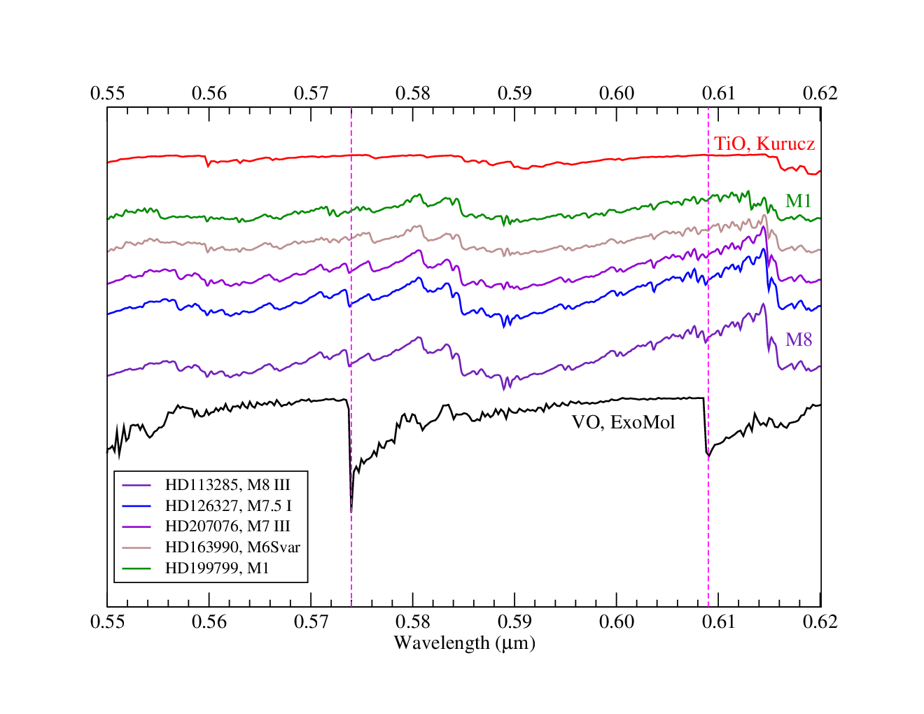
The top plot in Fig. 9 shows the spectra of M-type stars between 0.46 - 0.64 m (15,600 to 22,000 cm-1) against the new VO ExoMol line list and the pre-existing TiO linelist by Kurucz. The bottom plot is a zoomed-in view of the region from 0.56 to 0.61 m (16400 to 17,900 cm-1). The absorption by VO in this spectral region is dominated by the C-X transition bandheads. The top plot shows clearly that the main bandheads observed in the M-star spectra arise from TiO, not VO; this is expected as TiO is about an order of magnitude more abundant than VO. However, at approximately 0.548, 0.574 and 0.609 m, the VO bandheads become strong while there are weak or non-existent nearby TiO bandheads. In this regions, spectral absorption features in the M-type spectra do align well with the strong VO bandheads. This is further confirmed by the depth of this absorption feature as the spectral class changes from early M-type to late M-type stars (top to bottom). The absorption feature is significantly more pronounced for the cooler star. This aligns with the fact that late M-type stars have more VO than early M-type stars (in fact, the presence of VO absorption bands is one of the characterising spectral features of late M-type stars).


Fig. 10 compares the cross-section in the B-X region from the new VOMYT linelist against stellar spectra. The top plot is the B-X 1-0 band in the region 0.72 to 0.77 m (12,990 to 13,890 cm-1). Note that the M-star spectra are total cross-section, including a black-body contribution that rises steeply in this spectral region, whereas the ExoMol cross-section is a pure absorption spectra on a fixed intensity background. It is expected that the M8 star contains significant VO absorption features which are weak or non-existent in the M4 spectra. This is indeed what is observed. The agreement in the region 0.73 to 0.75 m is particularly strong. This corresponds to the B-X 1-0 band. The blackbody background is probably responsible for at least some of the differences from 0.75 to 0.758 m, while the difference in the 0.758 to 0.764 m is probably caused by absorption by another molecule.
The middle plot is the 0-0 band, centered around 0.79 m (12660 cm-1). This figure compares the VO ExoMol cross-section against the spectra of a late M-type star in the region 0.783 to 0.81 m (12,770 to 12,350 cm-1). The absorption peaks in the stellar spectra and the VOMYT cross-section are extremely similar, giving high confidence to our VOMYT linelist.
Finally, the bottom plot of Fig. 10 is the B-X 0-1 band with origin around 0.862 m. This figure compares the VOMYT cross-section at 3000 K against the spectra of a M7 and M8 star in the region 0.844 to 0.890 m (11,230 to 11,850 cm-1). Some features clearly align between the VOMYT and stellar spectra, as indicated by the vertical lines.


Figure 11 compares the VOMYT VO cross-section against stellar spectra in the region of the A-X 0-1 (top), 0-0 (middle) and 1-0 (bottom) bands. Considering first the middle subplot (the 0-0 band). The first major peak in the VO cross-section at around 1.046 m aligns well with a bump in the M9 spectral absorption, though there is obviously another species causing a nearby strong absorption at 1.046 m. The other peaks of the VO spectra all align reasonably well or at least are not inconsistent with the M9 stellar spectra, though there is again many other absorption peaks in this region. Note that the M2 and M3 stellar spectra seem reasonably featureless in this region and their absorption features do not coincide with VO’s (as expected). The M2 and M3 absorption features do seem roughly correlated with some other absorption in the M9 stellar spectra.
The top subplot of Fig. 11 covers the 0-1 band region and shows similar characteristics to the 0-0 band; the VOMYT absorption features are present in (or consistent with) the M9 but not the M2/M3 spectra and there are many other absorption features in the M9 and M2/M3 spectra that do not arise from VO absorption, but probably a different molecule.
The bottom subplot of Fig. 11 covers the VO 1.2 m band. There is little experimental data on the vibrationally excited A state (only a tentative assignment of the vibrational frequency). Despite this, the agreement between the stellar spectra and the VO linelist is reasonably good. The shape of the band is well reproduced and identification of the spectral features that can be attributed to VO are relatively clear. However, the positions of the spectral lines is somewhat in error (on order 10 Å, around 10 cm-1). This is about the expected error of this band and is a good indicator of the quality of this line list where direct experimental frequency measurements are not available, e.g. many hot and overtone bands.
Thus, our comparisons in Fig. 9, 10 and 11 show that the VO absorption features from our ExoMol cross-sections are consistent in the major bands to absorption in the late M-type stars, while VO absorption features are absent in the early M-type stars, as expected.


| Plez (1999) | Kurucz (2011) | VOMYT | |
| # Electronic States | 4 | 4 | 13 |
| Max | 15 | 15 | 59 |
| Max J | 199.5 | 199.5 | 197.5 |
| Max Energy (cm-1) | 42,387 | 50,000 | |
| Min Freq. (cm-1) | 3,767 | 0.537 | 0.01 |
| Max Freq. (cm-1) | 25,939 | 28,096 | 35,000 |
| Min WaveLength (m) | 0.386 | 0.355 | 0.2857 |
| Max WaveLength (m) | 2.655 | 18627.4 | 1,000,000 |
| Number of lines | 3,171,552 | 4,509,519 | 277,131,624 |
The characteristics of the Kurucz (2011), Plez (1999) and new ExoMol VOMYT linelists are summarised in Table 19. Note that even though the Kurucz line list has very low frequency transitions, all transitions are electronic; the infrared rovibrational transitions within the X state are not included. It is clear that the new VOMYT linelist is significantly more complete, with more than 60 times more lines covering both shorter and longer wavelengths than either of the previous line lists. There are more electronic states considered, and more vibrational energy levels. The maximum rotational quantum number is slightly lower due to the fact we used a lower energy cut-off to exclude all spectral lines originating from initial energies greater than 20,000 cm-1.
Use of our partition function suggests that the Kurucz and Plez line lists are 90% complete at 2800 K, but fall to approximately 50% complete by 5000 K. This incompleteness means that for high temperatures significant sources of opacity will be missing. The Plez line list has used extensively in models of hot Jupiters, brown dwarfs and cold stars, eg. by Plez (1999) as well as within the MARCS (Gustafsson et al., 2008), PHOENIX (Jack et al., 2009) and VSTAR (Bailey & Kedziora-Chudczer, 2012) modelling programs.
Fig. 12 compares the Plez, Kurucz and ExoMol VOMYT line lists in the regions 0.3 and 5 m. It is clear that the three line lists are broadly similar shorter than about 2 m, though the ExoMol VOMYT linelist extends to shorter wavelengths (and thus more to the blue). However, there are noticeable differences in intensities. For the A-X bands around 1 m, the Kurucz linelist is significantly stronger than either the Plez or ExoMol VOMYT line lists. The three line lists have similar strengths around the B-X bands, though the ExoMol line list is generally strongest especially at regions far from the bandhead; this is expected as it is most complete. The ExoMol VOMYT line list has stronger transitions in the C-X bands than either the Kurucz or Plez line lists.
Looking to the longer wavelength regions, the Plez line list does not represent the region longer than 2 m well. The Kurucz linelist is better with some features, but the ExoMol VOMYT linelist is significantly more complete. This is because the ExoMol linelist for the first time includes transitions from other electronic states, and from excited electronic states. The additional infrared absorption of VO described by our new line list may be important for energy transport and the spectroscopy of stellar and planetary atmospheres which contain VO molecule.


Figure 13 identifies the main bands in the absorption spectra of VO at 2200 K. The strongest microwave and infrared bands are about three orders of magnitude weaker than the strongest visible bands. In visible spectral region, the C-X transition has an inherently stronger intensity than the B-X transition, which is stronger than the A-X transition. It is clear that the A-X, B-X and C-X transitions contribute almost all of the opacity above 7000 cm-1 (below 1.4 m). At low frequencies (longer wavelengths), there are a significant number of contributing transitions, particularly the e-c, B-A and X-X transitions.

The importance of these non-ground electronic states can be quantified by considering the thermal distribution of initial states in an ensemble of VO molecules. Fig. 14 shows the relative population of excited states as a function of temperature. At 2000 K, only 2% of molecules are in excited states; by 5000 K, this increases to almost 45%! Furthermore, there are many excited states that are populated significantly; though the A′ state have the highest population (15%), there is significant population (above 1%) in six other excited states.
Our calculated transitions associated with the ground state will generally be more reliable than transitions that occur between excited states. This is due to existing experimental data. For example, for the a state is not well known experimentally and thus the frequencies of all transitions from this state have inherent large uncertainties. Limitations in the accuracy of the ab initio calculations also needs to be considered; low lying states are generally described more accurately than higher electronic states.
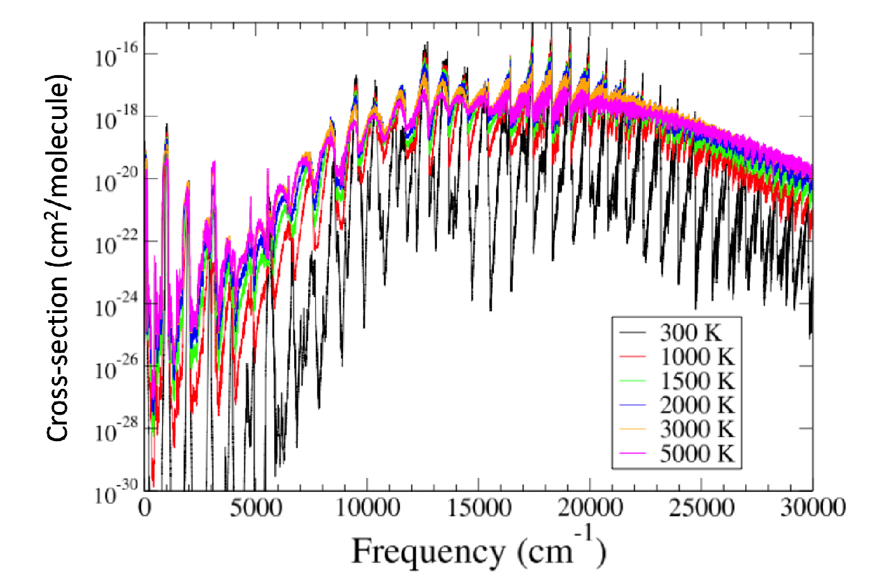
Fig. 15 shows the absorption spectra as a function of temperature. At higher temperatures, the structure of the spectra becomes less defined and broader, as expected.
5 Conclusion
Transition metal diatomics are important species in cooler stars and hot Jupiters. However, the difficulty of the ab initio calculations and the relative lack of experimental data mean that it is difficult to construct high quality line lists for these species.
Here we present the first ExoMol line list for a transition metal diatomic species of astrophysical relevance. Work on CrH, MnH and TiH is in advanced stages and will be published shortly. Using the lessons from the construction of the VO line list, we are now actively working on an improved high quality line list for TiO to address much discussed shortcomings in the existing line list in terms of intensities and at very high resolution. This new TiO line list will use high quality ab initio results and be fitted to all available experimental data. Furthermore, a Marvel-type analysis (Furtenbacher et al., 2007) is currently underway to extract high quality experimental energies from experimental frequencies.
Our VOMYT rovibronic line list for VO, containing over 277 million transitions, can be accessed online at www.exomol.com in the extended ExoMol format described by Tennyson et al. (2016b). It includes the transition energies and Einstein coefficients, partition functions, lifetimes and temperature-dependent cross-sections. Landé g factors to describe the splitting of the energy levels due to the Zeeman effect will be added shortly. We have also included the Duo input file with our spectroscopic model for VO.
Acknowledgements
This work is supported by ERC Advanced Investigator Project 267219. The authors acknowledge the use of the UCL Legion High Performance Computing Facility (Legion@UCL), and associated support services, in the completion of this work. Thanks to Joanna Barstow, Adam Burgasser, Jane MacArthur, August Muench and Hannah Wakeford for recommending good sources of astronomical data to compare against our linelist’s predictions.
References
- Adam et al. (1995) Adam A. G., Barnes M., Berno B., Bower R. D., Merer A. J., 1995, J. Mol. Spectrosc., 170, 94
- Agúndez et al. (2014) Agúndez M., Parmentier V., Venot O., Hersant F., Selsis F., 2014, A&A, 564, A73
- Allard & Hauschildt (1995) Allard F., Hauschildt P. H., 1995, ApJ, 445, 433
- Alvarez & Plez (1998) Alvarez R., Plez B., 1998, A&A, 330, 1109
- Bailey & Kedziora-Chudczer (2012) Bailey J., Kedziora-Chudczer L., 2012, MNRAS, 419, 1913
- Bakalbassis et al. (1996) Bakalbassis E. G., Stiakaki M. A. D., Tsipis A. C., Tsipis C. A., 1996, Chem. Phys., 205, 389
- Balabanov & Peterson (2005) Balabanov N. B., Peterson K. A., 2005, J. Chem. Phys., 123, 064107
- Balducci et al. (1983) Balducci G., Gigli G., Guido M., 1983, J. Chem. Phys., 79, 5616
- Bande & Lüchow (2008) Bande A., Lüchow A., 2008, Phys. Chem. Chem. Phys., 10, 3371
- Barklem & Collet (2016) Barklem P. S., Collet R., 2016, A&A, 588, A96
- Barstow et al. (2015) Barstow J. K., Aigrain S., Irwin P. G. J., Kendrew S., Fletcher L. N., 2015, MNRAS, 448, 2546
- Bauschlicher & Langhoff (1986) Bauschlicher C. W., Langhoff S. R., 1986, J. Chem. Phys., 85, 5936
- Bauschlicher & Maitre (1995) Bauschlicher C. W., Maitre P., 1995, Theor. Chim. Acta, 90, 189
- Beichman et al. (2014) Beichman C. et al., 2014, PASP, 126, 1134
- Bernath (2009) Bernath P. F., 2009, Int. Rev. Phys. Chem., 28, 681
- Bowler et al. (2010) Bowler B. P., Liu M. C., Dupuy T. J., Cushing M. C., 2010, ApJ, 723, 850
- Bridgeman & Rothery (2000) Bridgeman A. J., Rothery J., 2000, J. Chem. Soc. Dalton, 211
- Broclawik & Borowski (2001) Broclawik E., Borowski T., 2001, Chem. Phys. Lett., 339, 433
- Burrows et al. (1989) Burrows A., Hubbard W., Lunine J. I., 1989, ApJ, 345, 939
- Carlson & Moser (1966) Carlson K. D., Moser C., 1966, J. Chem. Phys., 44, 3259
- Castelaz et al. (2000) Castelaz M., Luttermoser D., Piontek R., 2000, ApJ, 538, 341
- Cenarro et al. (2001) Cenarro A., Cardiel N., Gorgas J., Peletier R., Vazdekis A., Prada F., 2001, MNRAS, 326, 959
- Cheung et al. (1994) Cheung A. S. C., Hajigeorgiou P. G., Huang G., Huang S. Z., Merer A. J., 1994, J. Mol. Spectrosc., 163, 443
- Cheung et al. (1981) Cheung A. S. C., Hansen R. C., Lyyra A. M., Merer A. J., 1981, J. Mol. Spectrosc., 86, 526
- Cheung et al. (1982a) Cheung A. S. C., Hansen R. C., Merer A. J., 1982a, J. Mol. Spectrosc., 91, 165
- Cheung et al. (1982b) Cheung A. S. C., Taylor A. W., Merer A. J., 1982b, J. Mol. Spectrosc., 92, 391
- Cushing et al. (2003) Cushing, M. C., Rayner, J. T., Vacca, W. D., 2005, ApJ, 623, 1115
- Dai et al. (2003) Dai B., Deng K., Yang J., Zhu Q., 2003, J. Chem. Phys., 118, 9608
- Désert et al. (2008) Désert J.-M., Vidal-Madjar A., Lecavelier des Etangs A., Sing D., Ehrenreich D., Hébrard G., Ferlet R., 2008, A&A, 492, 585
- Dolg et al. (1987) Dolg M., Wedig U., Stoll H., Preuss H., 1987, J. Chem. Phys., 86, 2123
- Dunning (1989) Dunning T. H., 1989, J. Chem. Phys., 90, 1007
- Evans et al. (2016) Evans T. M. et al., 2016, ApJ, 822, L4
- Falcón-Barroso et al. (2011) Falcón-Barroso J., Sánchez-Blázquez P., Vazdekis A., Ricciardelli E., Cardiel N., Cenarro A., Gorgas J., Peletier R., 2011, A&A, 532, A95
- Fortney et al. (2008) Fortney J. J., Lodders K., Marley M. S., Freedman R. S., 2008, ApJ, 678, 1419
- Fortney et al. (2010) Fortney J. J., Shabram M., Showman A. P., Lian Y., Freedman R. S., Marley M. S., Lewis N. K., 2010, ApJ, 709, 1396
- Furtenbacher et al. (2007) Furtenbacher T., Császár A. G., Tennyson J., 2007, J. Mol. Spectrosc., 245, 115
- Gibson et al. (2013) Gibson N. P., Aigrain S., Barstow J. K., Evans T. M., Fletcher L. N., Irwin P. G. J., 2013, MNRAS, 436, 2974
- Gustafsson et al. (2008) Gustafsson B., Edvardsson B., Eriksson K., Jorgensen U. G., Nordlund A., Plez B., 2008, A&A, 486, 951
- Harrington & Nicholls (1969) Harrington J., Nicholls R. W., 1969, J. Roy. Astron. Soc. Canada, 63, 208
- Haynes et al. (2015) Haynes K., Mandell A. M., Madhusudhan N., Deming D., Knutson H., 2015, ApJ, 806, 146
- Herczeg & Hillenbrand (2014) Herczeg G. J., Hillenbrand L. A., 2014, ApJ, 786, 97
- Hill et al. (2013) Hill C., Yurchenko S. N., Tennyson J., 2013, Icarus, 226, 1673
- Hocking et al. (1981) Hocking W. H., Merer A. J., Milton D. J., 1981, Can. J. Phys., 59, 266
- Hoeijmakers et al. (2015) Hoeijmakers H. J., de Kok R. J., Snellen I. A. G., Brogi M., Birkby J. L., Schwarz H., 2015, A&A, 575, A20
- Hopkins et al. (2009) Hopkins W. S., Hamilton S. M., Mackenzie S. R., 2009, J. Chem. Phys., 130, 144308
- Huang et al. (1992) Huang G. I., Merer A. J., Clouthier D. J., 1992, J. Mol. Spectrosc., 153, 32
- Huber & Herzberg (1979) Huber K. P., Herzberg G., 1979, Molecular Spectra and Molecular Structure IV. Constants of Diatomic Molecules. Van Nostrand Reinhold Company, New York
- Hübner et al. (2015) Hübner O., Hornung J., Himmel H.-J., 2015, J. Chem. Phys., 143, 024309
- Huitson et al. (2012) Huitson C. M., Sing D. K., Vidal-Madjar A., Ballester G. E., Lecavelier des Etangs A., Désert J.-M., Pont F., 2012, MNRAS, 422, 2477
- Jack et al. (2009) Jack D., Hauschildt P. H., Baron E., 2009, A&A, 502, 1043
- Karlsson et al. (1997) Karlsson L., Lindgren B., Lundevall C., Sassenberg U., 1997, J. Mol. Spectrosc., 181, 274
- Kasai (1968) Kasai P. H., 1968, J. Chem. Phys., 49, 4979
- Keenan & Schroeder (1952) Keenan P. C., Schroeder L. W., 1952, ApJ, 115, 82
- Kirkpatrick et al. (2006) Kirkpatrick J. D., Barman T. S., Burgasser A. J., McGovern M. R., McLean I. S., Tinney C. G., Lowrance P. J., 2006, ApJ, 639, 1120
- Kirkpatrick et al. (1993) Kirkpatrick J. D., Kelly D. M., Rieke G. H., Liebert J., Allard F., Wehrse R., 1993, ApJ, 402, 643
- Knowles & Werner (1988) Knowles P. J., Werner H.-J., 1988, Chem. Phys. Lett., 145, 514
- Knowles & Werner (1992) Knowles P. J., Werner H.-J., 1992, Theor. Chem. Acc., 84, 95
- Kuiper et al. (1947) Kuiper G. P., Wilson W., Cashman R. J., 1947, ApJ, 106, 243
- Kulik & Marzari (2010) Kulik H. J., Marzari N., 2010, J. Chem. Phys., 133, 114103
- Kurucz (2011) Kurucz R. L., 2011, Can. J. Phys., 89, 417
- Laud & Kalsulka (1968) Laud B. B., Kalsulka D. R., 1968, Indian J Phys, 42, 61
- Lee et al. (1999) Lee E. G., Seto J. Y., Hirao T., Bernath P. F., Le Roy R. J., 1999, J. Mol. Spectrosc., 194, 197
- Lodi et al. (2015) Lodi L., Yurchenko S. N., Tennyson J., 2015, Mol. Phys., 113, 1559
- Mackrodt et al. (2004) Mackrodt W. C., Middlemiss D. S., Owens T. G., 2004, Phys. Rev. B, 69, 115119
- Madhusudhan & Seager (2010) Madhusudhan N., Seager S., 2010, ApJ, 725, 261
- McGovern et al. (2004) McGovern M. R., Kirkpatrick J. D., McLean I. S., Burgasser A. J., Prato L., Lowrance P. J., 2004, ApJ, 600, 1020
- McKemmish et al. (2016) McKemmish L. K., Yurchenko S. N., Tennyson J., 2016, Mol. Phys. (submitted)
- Merer (1989) Merer A., 1989, Annu. Rev. Phys. Chem., 40, 407
- Merer et al. (1987) Merer A. J., Huang G., Cheung A. S. C., Taylor A. W., 1987, J. Mol. Spectrosc., 125, 465
- Miliordos & Mavridis (2007) Miliordos E., Mavridis A., 2007, J. Phys. Chem. A, 111, 1953
- Parmentier et al. (2013) Parmentier V., Showman A. P., Lian Y., 2013, A&A, 558, A91
- Patrascu et al. (2014) Patrascu A. T., Hill C., Tennyson J., Yurchenko S. N., 2014, J. Chem. Phys., 141, 144312
- Patrascu et al. (2015) Patrascu A. T., Tennyson J., Yurchenko S. N., 2015, MNRAS, 449, 3613
- Peterson et al. (2008) Peterson D. E. et al., 2008, ApJ, 685, 313
- Plez (1998) Plez B., 1998, A&A, 337, 495
- Plez (1999) Plez B., 1999, in Asymptotic Giant Branch Stars, Vol. 191, p. 75
- Pradhan et al. (2011) Pradhan K., Gutsev G. L., Weatherford C. A., Jena P., 2011, J. Chem. Phys., 134, 144305
- Pykavy & van Wullen (2003) Pykavy M., van Wullen C., 2003, J. Phys. Chem. A, 107, 5566
- Quan et al. (2008) Quan D., Ling W., Xiao-Hong S., Hong-Yan W., Tao G., Zheng-He Z., 2008, Acta Chimica Sinica, 66, 23
- Quan et al. (2006) Quan D., Ling W., Xiao-Hong S., Tao G., 2006, Acta Phys. Sin., 55, 6308
- Rajpurohit et al. (2014) Rajpurohit A. S., Reylé C., Allard F., Scholz R. D., Homeier D., Schultheis M., Bayo A., 2014, A&A, 564, A90
- Rajpurohit et al. (2012) Rajpurohit A. S., Reylé C., Schultheis M., Allard F., Scholz R., Homeier D., 2012, in SF2A-2012: Proceedings of the Annual meeting of the French Society of Astronomy and Astrophysics, Boissier S., de Laverny P., Nardetto N., Samadi R., Valls-Gabaud D., Wozniak H., eds., pp. 383–388
- Ram & Bernath (2005) Ram R. S., Bernath P. F., 2005, J. Mol. Spectrosc., 229, 57
- Ram et al. (2002) Ram R. S., Bernath P. F., Davis S. P., Merer A. J., 2002, J. Mol. Spectrosc., 211, 279
- Rayner et al. (2009) Rayner J. T., Cushing M. C., Vacca W. D., 2009, ApJS, 185, 289
- Richards & Barrow (1968a) Richards D., Barrow R. F., 1968a, Nature, 219, 1244
- Richards & Barrow (1968b) Richards D., Barrow R. F., 1968b, Nature, 217, 842
- Ryabchikova et al. (2015) Ryabchikova T., Piskunov N., Kurucz R. L., Stempels H. C., Heiter U., Pakhomov Y., Barklem P. S., 2015, Physica Scripta, 90, 054005
- Sánchez-Blázquez et al. (2006) Sánchez-Blázquez P. et al., 2006, MNRAS, 371, 703
- Sauval & Tatum (1984) Sauval A. J., Tatum J. B., 1984, ApJS, 56, 193
- Schwarz et al. (2015) Schwarz H., Brogi M., de Kok R., Birkby J., Snellen I., 2015, A&A, 576, A111
- Schwenke (1998) Schwenke D. W., 1998, Faraday Discuss., 109, 321
- Sharp & Burrows (2007) Sharp C. M., Burrows A., 2007, Astrophys. J. Suppl. Ser., 168, 140
- Spiegel & Burrows (2013) Spiegel D. S., Burrows A., 2013, ApJ, 772, 76
- Spiegel et al. (2009) Spiegel D. S., Silverio K., Burrows A., 2009, ApJ, 699, 1487
- Spinrad & Wing (1969) Spinrad H., Wing R. F., 1969, ARA&A, 7, 249
- Spinrad & Younkin (1966) Spinrad H., Younkin R. L., 1966, PASP, 78, 65
- Sriramachandran et al. (2008) Sriramachandran P., Bagare S. P., Rajamanickam N., Balachandrakumar K., 2008, Sol. Phys., 252, 267
- Suenram et al. (1991) Suenram R. D., Fraser G. T., Lovas F. J., Gillies C. W., 1991, J. Mol. Spectrosc., 148, 114
- Tennyson (2014) Tennyson J., 2014, J. Mol. Spectrosc., 298, 1
- Tennyson et al. (2013) Tennyson J., Hill C., Yurchenko S. N., 2013, in AIP Conference Proceedings, Vol. 1545, 6th international conference on atomic and molecular data and their applications ICAMDATA-2012, AIP, New York, pp. 186–195
- Tennyson et al. (2016a) Tennyson J., Lodi L., McKemmish L. K., Yurchenko S. N., 2016a, J. Phys. B: At. Mol. Opt. Phys., 49, 102001
- Tennyson & Yurchenko (2016) Tennyson J., Yurchenko S., 2016, Exp. Astron., 40, 563
- Tennyson & Yurchenko (2012) Tennyson J., Yurchenko S. N., 2012, MNRAS, 425, 21
- Tennyson & Yurchenko (2014) Tennyson J., Yurchenko S. N., 2014, in IAU Symposium, Vol. 297, The diffuse interstellar bands, Cami J., Cox N. L. J., eds., pp. 330–338
- Tennyson et al. (2016b) Tennyson J. et al., 2016b, J. Mol. Spectrosc. (in press), https://arxiv.org/abs/1603.05890
- Tinetti et al. (2012) Tinetti G. et al., 2012, Exp. Astron., 34, 311
- Tinetti et al. (2011) Tinetti G. et al., 2011, in IAU Symposium Proceedings Series, Vol. 276, Astrophysics of Planetary Systems: Formation, Structure, and Dynamical Evolution, Sozzetti A., Lattanzi M., Boss A., eds., pp. 359–370, 276th Symposium of the International-Astronomical-Union on Astrophysics of Planetary Systems: Formation, Structure, and Dynamical Evolution, Torino, ITALY, OCT 10-15, 2010
- Šurkus et al. (1984) Šurkus A. A., Rakauskas R. J., Bolotin A. B., 1984, Chem. Phys. Lett., 105, 291
- Wakeford & Sing (2015) Wakeford H. R., Sing D. K., 2015, A&A, 573, A122
- Werner & Knowles (1988) Werner H., Knowles P. J., 1988, J. Chem. Phys., 89, 5803
- Werner et al. (2012) MOLPRO-WIREs Werner H.-J., Knowles P. J., Knizia G., Manby F. R., Schütz M., et al., 2012, WIREs Comput Mol Sci, 2, 242
- Western (2016) Western C. M., 2016, J. Quant. Spectrosc. Radiat. Transf., (in press), doi:10.1016/j.jqsrt.2016.04.010
- Wing et al. (1967) Wing R. F., Spinrad H., Kuhi L., 1967, ApJ, 147, 117
- Wolf et al. (1977) Wolf G. V., Farberov D. S., Shirokovskii V. P., 1977, Intern. J. Quantum Chem., 12, 485
- Wu & Wang (1998) Wu H. B., Wang L. S., 1998, J. Chem. Phys., 108, 5310
- Yao et al. (2007) Yao C., Guan W., Song P., Su Z. M., Feng J. D., Yan L. K., Wu Z. J., 2007, Theor. Chem. Acc., 117, 115
- Yurchenko et al. (2016a) Yurchenko S. N., Blissett A., Asari U., Vasilios M., Hill C., Tennyson J., 2016a, MNRAS, 456, 4524
- Yurchenko et al. (2016b) Yurchenko S. N., Lodi L., Tennyson J., Stolyarov A. V., 2016b, Comput. Phys. Commun., 202, 262