Glue spin and helicity in proton from lattice QCD
![[Uncaptioned image]](1609.05937v3/figures/chiqcd.png) (QCD Collaboration)
(QCD Collaboration)
Abstract
We report the first lattice QCD calculation of the glue spin in the nucleon. The lattice calculation is carried out with valence overlap fermions on 2+1 flavor DWF gauge configurations on four lattice spacings and four volumes including an ensemble with physical values for the quark masses. The glue spin in the Coulomb gauge in the scheme is obtained with the 1-loop perturbative matching. We find the results fairly insensitive to lattice spacing and quark masses. We also find that the proton momentum dependence of in the range GeV is very mild, and we determine it in the large momentum limit to be at the physical pion mass in the scheme at GeV2. If the matching procedure in large momentum effective theory is neglected, is equal to the glue helicity measured in high-energy scattering experiments.
Introduction: Deep-inelastic scattering experiments reveal that contrary to the naive quark model, the quark spin contribution to the proton spin is quite small, about 30 [1, 2, 3]. In an effort to search for the missing proton spin, recent analyses [4, 5] of the high-statistics 2009 STAR [6] and PHENIX [7] experiments at RHIC showed evidence of non-zero glue helicity in the proton. For GeV2, the glue helicity distribution is found to be positive and away from zero in the momentum fraction region . However, the results are limited by very large uncertainty in this region.
The recent COMPASS analysis explored from the scaling violation of , and the highly distinct solutions of can be obtained with different parameterizations of [8]. Therefore, it hints that if a high precision can be obtained directly, it will benefit our understanding of the parameterizations of and provide more information about the role of quark spin in the proton.
Given the importance of to explain the origin of the proton spin, and the fact that significant efforts are devoted to its precise experimental determination, a theoretical understanding and calculation of is highly desired. is defined as the first moment of the glue helicity distribution [9],
| (1) | |||||
where the light front coordinates are . The proton plane wave state is written as , with momentum and polarization . The light-cone gauge-link is defined in the adjoint representation. It connects the gauge field tensor and its dual, , to construct a gauge invariant operator. After integrating over , one can define the gauge-invariant gluon helicity operator in a non-local form [10, 11],
| (2) |
where . It is the gauge-invariant extension (GIE) of the operator in the light-cone gauge , but one cannot evaluate this expression on the lattice directly due to its real-time dependence.
On the other hand, is equal to the infinite momentum frame (IMF) limit of a universality class of operators [12] whose matrix elements can be matched to through a factorization formula in large momentum effective theory (LaMET) [13, 14]. The gluon spin operator proposed in Ref. [15, 16] with the non-abelian transverse condition belongs to this universality class and has been proven to be equivalent to the GIE of in the Coulomb gauge [17, 18],
| (3) |
where the factor 2 is from the normalization of the group generators and and are the chromoelectric field and gauge potential in the Coulomb gauge with their lattice versions to be addressed in the following.
is not Lorentz covariant and has nontrivial frame dependence [11]. It is shown in Ref. [12] that when boosted to the IMF, the Coulomb gauge fixing condition (as well as the temporal condition ) [12] become , and then the longitudinal component of in either gauge is equivalent to the glue helicity operator with a proper matching to cancel the intrinsic frame dependence of . On the lattice, the Coulomb condition can be obtained numerically [19] and the glue spin operator in the Coulomb gauge can be calculated without numerical difficulty.
The major task of this work is calculating the matrix element of in the proton, which will be indicated as , in the rest and moving frames. The results are then renormalized at 1-loop order in lattice perturbation theory and matched to the scheme at =10 GeV2, to investigate their frame dependence and address the matching to the helicity.
Numerical details: A preliminary attempt [20] to calculate was carried out on flavor dynamical domain-wall configurations on a lattice (24I) with the sea pion mass at MeV and on a lattice with sea pion mass at 300 MeV [21]. In this work, we improve the statistics on the ensembles mentioned above and carry out the calculation on another three ensembles with different lattice spacings, volumes, and sea quark masses to check the corrections to the glue spin from various systematic uncertainties. We use the 2-2-2 smeared stochastic grid source on all the ensembles (except 48I where the 4-4-4 smeared stochastic grid source is used), and apply the low-mode substitution [22, 23] to make the signal-to-noise ratio close to that with 8 (64 on the 48I ensemble) independent smeared point sources. Furthermore, we loop over all the time slices for the two-point functions of the nucleon to increase statistics. The statistics used for this grid source measurements is roughly equivalent to evaluating a large number of quasi-independent smeared point source measurements ranging from 103,936 on the 24I lattice to 497,664 on the 48I lattice. The parameters of the ensembles used in this work are listed in Table 1 and more details of the simulation setups can be found in the supplemental materials [24].
| Symbol | (MeV) | |||
|---|---|---|---|---|
| 32ID | 0.1431(7) | 170 | 200 | |
| 48I | 0.1141(2) | 140 | 81 | |
| 24I | 0.1105(3) | 330 | 203 | |
| 32I | 0.0828(3) | 300 | 309 | |
| 32If | 0.0627(3) | 370 | 238 |
The Coulomb gauge fixing condition used here is enforced by requiring that the spatial sum of the backward difference of the HYP-smeared gauge links [26] to be zero,
| (4) |
where is the Coulomb gauge fixed Wilson link from to . The gauge fixed potential is defined by
| (5) |
with as the bare coupling constant, and the chromoelectric field used in this work is given by the clover definition
| (6) | |||||
where .
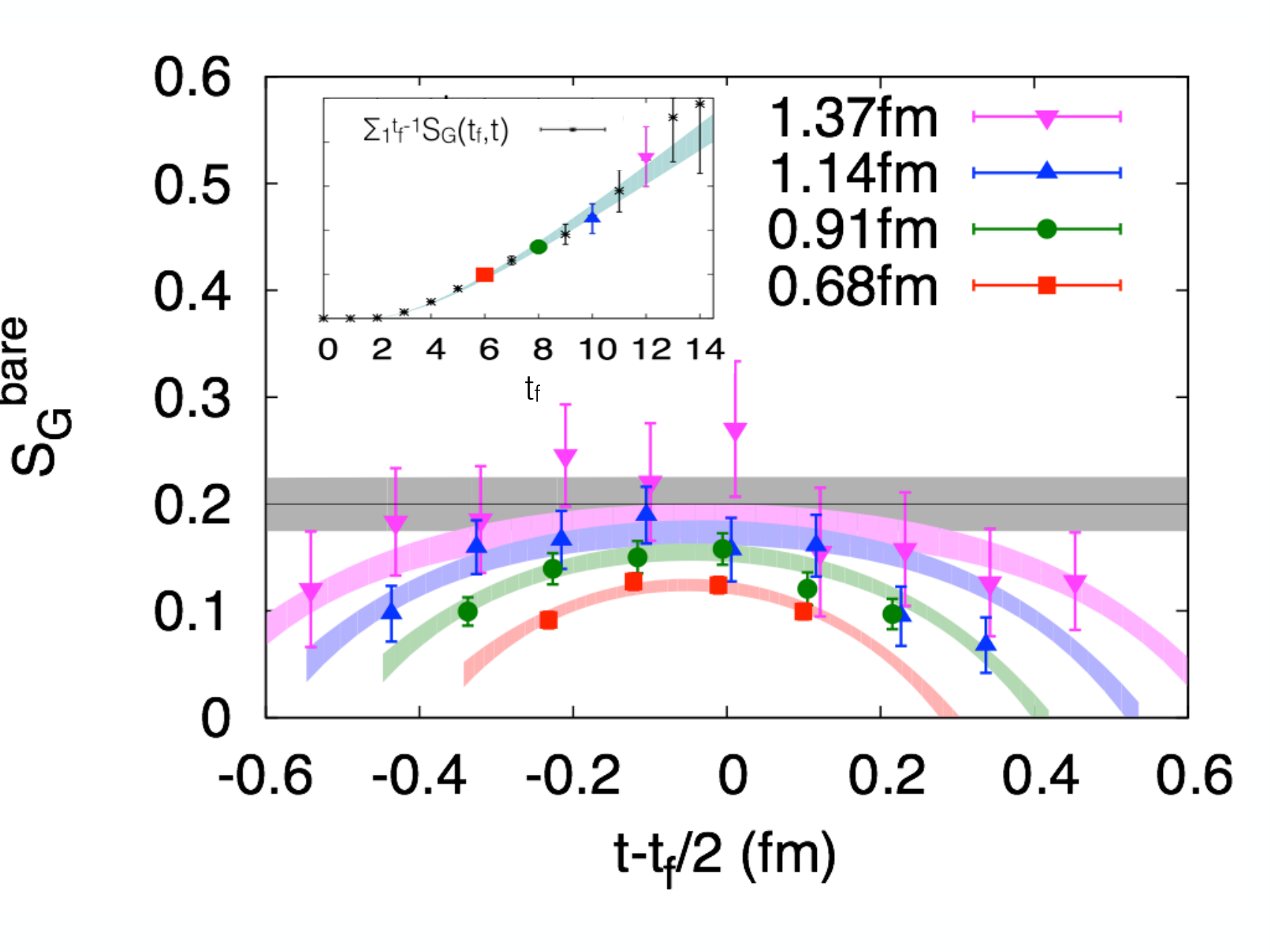
In order to extract , we compute the ratio of the disconnected three-point function with the gluon operator insertion to the nucleon propagator with the source and sink of the nucleon located at and , respectively. The glue spin operator is inserted at the time slice which is between and . Then the ratio in a moving frame along the -direction is
where is the nucleon interpolation field and and are the unpolarized projection operator of the proton and the polarized one along the -direction, respectively. When is large enough, is equal to the proton matrix element of the longitudinal glue spin operator, , plus -dependent corrections,
where is the energy difference between the first excited state and the ground state and are the spectral weights involving the excited state.
We plot the ratio for the unitary point on the 24I ensemble, as a function of for several in Fig. 1. The curves predicted by the fit agree with the data, and the /d.o.f is smaller than 1.4 for all the other quark masses on five ensembles. From the fit, we see that the excited-state contamination is small when the source-sink separation is larger than 1 fm. The final prediction of (the gray band) is consistent with the blue and purple data points at . Similar plots for the other ensembles can be found in the supplemental materials [24].
It is observed that the central values of the glue spin matrix elements as a function of HYP smearing steps are unchanged after two or three steps of smearing, as shown in Fig. 2 (for the case of the unitary point on the ensemble 24I), while the signal to noise ratio (SNR) can be improved when more HYP smearing steps are applied. In this work, 5 steps of HYP smearing are used for the glue spin operator on each ensemble, and the nucleon two-point correlators with the source located on all the time slices are generated to increase the SNR. Since the tadpole improvement factor is 2 for the operator without any HYP smearing, the enlargement of the result after the HYP smearing is understandable. Note that the HYP smearing here just affects the glue spin operator but the gauge action is unchanged since no reweighting is applied on configuration averages.
Results: The renormalized matrix element including mixing from the quark spin is [27]
| (9) | |||||
where the superscripts and indicate the quantities under the scheme and that under lattice regularization. We applied the Cactus improvement [28] to re-sum the major tadpole contributions to get a better convergence in the 1-loop correction of the glue spin. Then the re-summed finite piece depends on the bare coupling weakly and is in the range of 1.7–2.4 for the values of we used in this work. The details are addressed in Ref. [27]. Since the value of the mixing term involving in Eq. (9) is at the same order of the present statistical error of , the uncertainty due to for the gauge ensembles considered here will be even smaller. Therefore, we approximate the quark spin by the experimental value , which is 30% of the total proton spin from the global analysis of deep inelastic scattering data [1, 2, 3].
After matching to the values under the scheme at GeV2, we find that the valence quark mass dependence is mild regardless of the proton momentum. In Fig. 3, we show results in the rest frame for various valence quark masses on all the five ensembles, with five pairs of volumes and lattice spacings. Their dependence is also mild. To obtain in a relatively large momentum frame, we calculate for all the momenta smaller than on all the five ensembles. To show the frame dependence, we extrapolate on all the ensembles in different momentum frames to the physical value of the valence pion mass, as shown in Fig. 4. Some points are not shown in the figure if their uncertainties are larger than the signal.
The glue helicity in the proton, , corresponds to the glue longitudinal spin component in the IMF. The large-momentum effective field theory (LaEMT) [14], shows a large finite correction at the 1-loop level,
| (10) | |||||
At GeV2 and GeV the factor before is 0.22, which is much smaller than unity and indicates a convergence problem for the perturbative series even after one re-sums the large logarithms. (The factor is 0.80 if the finite piece 10.2098 is removed.) On the other hand, the largest momentum we have on the lattice with acceptable signal is comparable to the proton mass, so the power corrections in Eq. (10) cannot be neglected and one cannot simply apply this matching condition. Nevertheless, the mild dependence of on the proton momentum as in Fig. 4 leads us to suggest that it could be a small effect to match to the IMF, i.e., .
Therefore, we neglect the 1-loop LaMET matching and use the following empirical form to fit our data,
| (11) | |||||
where =0.139 GeV and GeV are the physical pion and proton mass respectively and are the valence and sea pion masses respectively. The correction in Eq. (10) is replaced by to include all the data in the fitting. Since all the coefficients other than are small, the cross terms and the higher-order terms are ignored. The overall /d.o.f. is 1.21 with 110 degrees of freedom. In Fig. 4, the band of the global fit with the empirical form in Eq. (11) shows that the frame dependence is mild and the central value is changed by less than 10% from its value in the rest frame to that at 1.5 GeV; the change is smaller than the statistical uncertainty.
Since the Coulomb gauge fixing on the lattice has a built-in correction, we repeated the fit with a linear term in . The central value is changed by about 1%, while the uncertainty is larger. We take the variance of the central values from two fits as an estimate of this uncertainty. Similarly, the uncertainty from the volume dependence is estimated in the same way and added to the systematic uncertainties in quadrature. In addition, the value of the quark spin is varied by 20% to cover the value 0.30 [1] and that from Ref. [3]. The final result is = 0.251(47)(16) with two errors from the statistical and systematic uncertainties.
Summary and outlook: In this work, we calculated the glue spin in the proton for the first time based on in the Coulomb gauge [15, 16], with various quark masses, lattice spacings, volumes, and proton momenta. The results show mild dependencies on these quantities. After 1-loop perturbative matching from the lattice theory to the continuum and neglecting the matching effect between the glue spin and helicity, we conclude that the gluon helicity , which is 50(9)(3)% of the total proton spin. The Cactus improvement [28] we used in Eq. (9) indicates that uncertainties can be considerable in perturbative QCD, and its reliability should be checked with non-perturbative renormalization in the future.
On the LaMET side, the convergence problem warrants the matching condition to be calculated at the 2-loop level or higher. On the other hand, if the glue spin in the temporal gauge can be calculated on the lattice, then its LaMET matching in Eq. (10) can be avoided at the 1-loop level [12]. This possibility is worthy of further investigation [27].
ACKNOWLEDGMENTS
We thank X. D. Ji and F. Yuan for useful comments and the RBC and UKQCD collaborations for providing us their DWF gauge configurations. This work is supported in part by the U.S. DOE Grant No. DE-SC0013065. A.A. is supported in part by the National Science Foundation CAREER grant PHY- 1151648 and by U.S. DOE Grant No. DE-FG02-95ER40907. Y. Z. is supported in part by the U.S. Department of Energy Office of Science, Office of Nuclear Physics under Award Number DE-FG02-93ER-40762 and DE-AC02-05CH11231. Y. Y. also thanks the Institute of High Energy Physics, Chinese Academy of Science for its partial support and hospitality. This material is based upon work supported by the U.S. Department of Energy, Office of Science, Office of Nuclear Physics, within the framework of the TMD Topical Collaboration. This research used resources of the Oak Ridge Leadership Computing Facility at the Oak Ridge National Laboratory, which is supported by the Office of Science of the U.S. Department of Energy under Contract No. DE-AC05-00OR22725. This work also used the Extreme Science and Engineering Discovery Environment (XSEDE), which is supported by National Science Foundation grant number ACI-1053575.
Supplemental materials
.1 The simulation setup
For the nucleon propagators, a regular grid with 2 smeared sources in each spatial direction for the 24I, 32I, 32ID and 32If lattices (4 for the 48I lattice since it has a much large volume) are placed on each of 2 time slices for the 24I, 32I and 32ID lattices (3 for the 48I lattice and 1 for the 32If lattice due to the different sizes in the time direction). We loop over all the time slices for the nucleon source. The position of the grid is randomly shifted on each time slice.
On the 32ID and 32If ensembles, we use the smeared sink to reduce the excited-states contamination from the sink side. The setup of the nucleon propagators simulation are summarized in Table. 2
| Ensemble | 24I | 32I | 48I | 32ID | 32If |
| Volume (fm4) | |||||
| (fm) | 0.55 | 0.56 | 0.56 | 0.50 | 0.48 |
| (fm) | 0 | 0 | 0 | 0.50 | 0.48 |
.2 The fit of the ratio
The functional form of the summed ratio
| (12) |
can be obtained from that of the ratio
| (13) |
where is the energy difference between the first excited-state and the ground state, and are the spectral weights involving the excited-states.
The standard summation method [23] approximates as
| (14) |
where all the terms proportional to in Eq. (12) are dropped. This introduces a systematic uncertainty when is not very large. At the same time, the classic plateau method cannot distinguish the term in Eq. (13) from the matrix element we want, except when the calculations are repeated with several values of . The two-state method can be more reliable than the summation method since it can make use all the information of , not just their sum over .
As a cross check, we plot the summed ratio together with the original plot of the ratios for the case of MeV on all the ensembles in Figs. 5-9. In the right panels of these figures, the four colored points correspond to the sum of the ratios at four different which are shown in the left panels. The bands in the right panels show the prediction of based on the two-state fits in Eq. 13. The data points agree with the gray band very well at larger .
For the cases on the 32ID and 32If ensembles in which the sink smearing is applied (Fig. 8 and Fig. 9), the curvatures as a function of are symmetric within uncertainty on both sides of , while those on the other ensembles are not expected to be symmetric. The excited-state contaminations are slightly larger on the 32ID and 32If ensembles since the effective smearing sizes are smaller compared to those on the other ensembles.
References
- [1] A. Accardi et al., Eur. Phys. J. A52, 268 (2016), arXiv:1212.1701 [nucl-ex] .
- [2] D. de Florian, R. Sassot, M. Stratmann, and W. Vogelsang, Phys. Rev. D80, 034030 (2009), arXiv:0904.3821 [hep-ph] .
- [3] C. A. Aidala, S. D. Bass, D. Hasch, and G. K. Mallot, Rev. Mod. Phys. 85, 655 (2013), arXiv:1209.2803 [hep-ph] .
- [4] D. de Florian, R. Sassot, M. Stratmann, and W. Vogelsang, Phys. Rev. Lett. 113, 012001 (2014), arXiv:1404.4293 [hep-ph] .
- [5] E. R. Nocera, R. D. Ball, S. Forte, G. Ridolfi, and J. Rojo (NNPDF), Nucl. Phys. B887, 276 (2014), arXiv:1406.5539 [hep-ph] .
- [6] P. Djawotho (STAR), Proceedings, 3rd Workshop on the QCD Structure of the Nucleon (QCD-N’12), Nuovo Cim. C036, 35 (2013), arXiv:1303.0543 [nucl-ex] .
- [7] A. Adare et al. (PHENIX), Phys. Rev. D90, 012007 (2014), arXiv:1402.6296 [hep-ex] .
- [8] C. Adolph et al. (COMPASS), Phys. Lett. B753, 18 (2016), arXiv:1503.08935 [hep-ex] .
- [9] A. V. Manohar, Phys. Lett. B255, 579 (1991).
- [10] Y. Hatta, Phys. Rev. D84, 041701 (2011), arXiv:1101.5989 [hep-ph] .
- [11] X. Ji, J.-H. Zhang, and Y. Zhao, Phys. Rev. Lett. 111, 112002 (2013), arXiv:1304.6708 [hep-ph] .
- [12] Y. Hatta, X. Ji, and Y. Zhao, Phys. Rev. D89, 085030 (2014), arXiv:1310.4263 [hep-ph] .
- [13] X. Ji, Sci. China Phys. Mech. Astron. 57, 1407 (2014), arXiv:1404.6680 [hep-ph] .
- [14] X. Ji, J.-H. Zhang, and Y. Zhao, Phys. Lett. B743, 180 (2015), arXiv:1409.6329 [hep-ph] .
- [15] X.-S. Chen, X.-F. Lu, W.-M. Sun, F. Wang, and T. Goldman, Phys. Rev. Lett. 100, 232002 (2008), arXiv:0806.3166 [hep-ph] .
- [16] X.-S. Chen, W.-M. Sun, X.-F. Lu, F. Wang, and T. Goldman, Phys. Rev. Lett. 103, 062001 (2009), arXiv:0904.0321 [hep-ph] .
- [17] C. Lorce, Phys. Rev. D87, 034031 (2013), arXiv:1205.6483 [hep-ph] .
- [18] Y. Zhao, K.-F. Liu, and Y. Yang, Phys. Rev. D93, 054006 (2016), arXiv:1506.08832 [hep-ph] .
- [19] M. Schröck and H. Vogt, Comput. Phys. Commun. 184, 1907 (2013), arXiv:1212.5221 [hep-lat] .
- [20] R. S. Sufian, M. J. Glatzmaier, Y.-B. Yang, K.-F. Liu, and M. Sun (QCD), Proceedings, 32nd International Symposium on Lattice Field Theory (Lattice 2014), PoS LATTICE2014, 166 (2015), arXiv:1412.7168 [hep-lat] .
- [21] Y.-B. Yang, R. S. Sufian, A. Alexandru, T. Draper, M. J. Glatzmaier, and K.-F. Liu (QCD), Proceedings, 33rd International Symposium on Lattice Field Theory (Lattice 2015): Kobe, Japan, July 14-18, 2015, PoS LATTICE2015, 129 (2016), arXiv:1603.05256 [hep-ph] .
- [22] A. Li et al. (QCD), Phys. Rev. D82, 114501 (2010), arXiv:1005.5424 [hep-lat] .
- [23] M. Gong et al. (QCD), Phys. Rev. D88, 014503 (2013), arXiv:1304.1194 [hep-ph] .
- [24] Supplemental Materials .
- [25] T. Blum et al. (RBC, UKQCD), Phys. Rev. D93, 074505 (2016), arXiv:1411.7017 [hep-lat] .
- [26] A. Hasenfratz and F. Knechtli, Phys. Rev. D64, 034504 (2001), arXiv:hep-lat/0103029 [hep-lat] .
- [27] Y.-B. Yang and Y. Zhao, in preparation (2016).
- [28] M. Constantinou, H. Panagopoulos, and A. Skouroupathis, Phys. Rev. D74, 074503 (2006), arXiv:hep-lat/0606001 [hep-lat] .