Extremal storage functions and minimal realizations of discrete-time linear switching systems
Abstract
We study the induced gain of discrete-time linear switching
systems with graph-constrained switching sequences.
We first prove that, for stable systems in a minimal realization, for
every , the -gain is exactly
characterized through switching storage functions.
These functions are shown to be the th power of a norm.
In order to consider general systems, we provide an algorithm for computing minimal realizations.
These realizations are rectangular systems, with a state
dimension that varies according to the mode of the system.
We apply our tools to the study on the of -gain. We provide algorithms for its approximation, and provide a converse result for the existence
of quadratic switching storage functions. We finally illustrate the results with a physically motivated example.
I Introduction
Discrete-time linear switching systems are multi-modal systems that switch between a finite set of modes. They arise in many practical and theoretical applications [22, 16, 2, 17, 13, 31]. They are of the form
| (1) | ||||
where , and are respectively the state of the system,
a disturbance input, and a performance output. The function is called a switching sequence, and at time , is called the mode of the system at time . We consider switching sequences following a set of logical rules: they need be generated by walks in a given labeled graph (we will denote this by ).
The analysis and control of switched systems is an active research area, and many questions that are easy to understand and decide for LTI (i.e., Linear Time Invariant) systems are known to be hard for switching systems (see, e.g., [6, 16, 22, 29]). Nevertheless, several analysis and control techniques have been devised (see e.g. [21, 20, 19, 11]), often providing conservative yet tractable methods. The particular question of the stability of a switched system attracts a lot of attention; in the past few years, approaches using multiple Lyapunov functions have been devised [8, 4, 21], with recent works [28, 12, 1] analyzing how conservative these methods are.
In this paper, we are interested in the analysis and computation of the induced gain of switching systems:
| (2) |
where means that the disturbance signal satisfies , being the -norm of .
This quantity is a measure of a system’s ability to dissipate the energy of a disturbance.
As noted in [25], the -gain is one of the most studied performance measures. Some approaches link the gain of a switching system to the individual performances of its LTI modes (see e.g. [7, 14]); in [11, 20], a hierarchy of LMIs is presented to decide whether . In [30], a generalized version of the gain is studied through generating functions. For continuous time systems, [15] gives a tractable approach based on the computation of a storage function. For the general -gain, we refer to [24] that relies on an operator-theoretic approach.
Our approach is inspired from the works [28, 12, 1] on stability analysis. These works present a framework for the stability analysis of switching systems (with constrained switching sequences) using multiple Lyapunov functions with pieces that are norms. In Section II, we provide a characterization of -gain using multiple storage functions, where pieces are now the th power of norms. We rely on two assumptions, namely that
the switching system be internally stable and in a minimal realization. In order to assert the generality of the results, both assumptions are discussed in Subsections II-A and Subsection II-B respectively. In particular, we give an algorithm for computing minimal realizations: these are rectangular systems for which the dimension of the state space varies with the modes of the system. In Section III, we narrow our focus to the -gain, providing two approaches for estimating the gain and constructing storage functions. The first uses dynamic programming and provides asymptotically tight lower bound on the gain, while the second, based on the work of [11, 20], provides asymptotically tight upper bounds.
Then, in Subsection III-A we present a converse result for the existence of quadratic storage functions, which can be obtained using convex optimization.
Section IV illustrates our results with a simple practical example.
Preliminaries
Given a system of the form (1) on modes, we denote the set of parameters of the system by
We define constraints on the switching sequences through a strongly connected, labeled and directed graph (see e.g. [28, 19, 11]). The edges of are of the form , where are the source and destination nodes and is a label that corresponds to a mode of the switching system. A constrained switching system is then defined by a pair , and admissible switching sequences correspond to paths in (see Fig. 1 for examples).


More precisely, let denote a finite-length path in the graph. The associated switching sequence is written , where, for a given , is the label on the th edge of . The length of , i.e., the number of edges it contains, is written . We let with denote the path formed from the th edge of to its th (both included). We let be the sequence of nodes encountered by , where is the source node, and if , is the destination node. The functions and need not be defined for . In order to compactly describe the input-output maps of the system, we write
| (3) |
| (4) |
| (5) |
| (6) |
If is an infinite path, we define , , , and similarly, the last three being operators on .
When in a matrix, and are the null and identity matrix of appropriate dimensions.
Given a matrix , is the image of and the kernel of . The orthogonal of a subspace of is . The sum of subspaces of , , is
II Extremal storage functions
Our main results for this section rely on two assumptions. They are discussed in Subsections II-A and II-B.
Assumption 1 (Minimality)
This definition of minimality equivalent to that found in [26], Theorem 1. Minimality requires that any state has a reachable and a detectable component.
Assumption 2 (Internal stability)
The system is internally (exponentially) stable, i.e., there exist and such that
Internal stability guarantees that the -gain of the system is bounded (see e.g. [10]). It is difficult to decide whether a given constrained system is internally stable. Towards this end, generalizing the tools introduced in [1], the concept of multinorm is introduced in [28]:
Definition 1
A multinorm for a system is a set of one norm of per node in .
This concept allowed to develop tools for the approximation of the constrained joint spectral radius, denoted , of systems (see [9, 28]). It can be shown that the internal stability of a system is equivalent to (see e.g. [9, 18]), and in [28]-Proposition 2.2, the authors show that
| (8) |
Thus, a constrained switching system is stable if and only if it has a multiple Lyapunov function, with no more than one piece per node of , which can be taken as a norm. Whenever the infimum is actually attained by a multinorm, we say it is extremal. The existence of such an extremal multinorm is not guaranteed.
We now show that multinorms provide a characterization of the -gain of constrained switching systems. They play the role of multiple storage functions.
Moreover, there exists always an extremal multinorm acting as storage function for internally stable and minimal systems, i.e. that attains the value in (9).
Theorem II.2
Consider a system , an integer , and . At each node , define the function
| (11) |
The set of functions is an extremal multinorm, i.e., for all , and ,
| (12) | |||
Proofs of main results
Consider a system . We need to show that if holds, then . Then, proving Theorem 12 proves Theorem II.1. We know is bounded as a consequence of Assumption 2.
The first element is proven by simple algebra. Assume (10) holds, take , an infinite path , and a sequence . Unfolding the inequality, we obtain for all ,
Therefore, for all , and this being independent of and , we get . We now move onto the proof of Theorem 12. Proving (12) is easy, so we focus on proving that for , the functions are norms. We omit the subscripts and in what follows. The functions have the following properties:
- 1.
Observe that , taking a disturbance . Assume by contradiction that there is such that . There must be a path and a sequence such that
Thus, (see (2)), a contradiction.
- 2.
is positive definite. By Assumption 1, for any node , for any , there is a path , , such that . Thus, is guaranteed by taking .
- 3.
is convex and positively homogeneous of order . Given a path of finite length, define the output sequence
Clearly, for any . Therefore, for any , , we have
Since is convex in , the convexity of is then easily proven.
- 4.
. Take for some with , . Let , and let be such that . We have that
and thus is bounded. Now, take any . By Assumption 1, we know that is a linear combination of points in the reachable sets , Thus, by convexity, .
We discuss the generality of the Assumptions 1 and 2 in the next subsections.
II-A Internal stability or undecidability
Assumption 2 is a sufficient condition for , which is key in Theorems II.1 and 12. Relaxing the assumption leads to decidability issues:
Proposition II.3
Given a switching system and , the question of whether or not is undecidable.
Proof:
Consider an arbitrary switching system on two modes, with and for . The undecidability result presented in [6] states that the question of the existence of a uniform bound such that, for all and all , the products of matrices satisfy , is undecidable. We show that as a consequence, one cannot in general decide the boundedness of the gain of a (constrained) switching system. Given a pair of matrices, construct an arbitrary switching system of the form (1) on 3 modes with the parameters Σ= {{A_1,0,0,0}, {A_2,0,0,0}, {0,I,I,0}}, with input and output dimension . Then, the -gain of this system is given by γ_p(Θ, Σ) = w 0 , T, σ(0), …, σ(T-1) ∈{1,2} T sup ∥A σ(T-1) ⋯A σ(0) w 0 ∥ p ∥w 0 ∥ p . Thus, the gain of the system is bounded if and only if there is a uniform bound on the norm of all products of matrices from the pair . ∎
II-B Obtaining minimal realizations.
We now turn our attention to Assumption 1.
Section IV presents a practically motivated system for which a very natural model turns out to be non-minimal. We need to provide a minimal realization for the system. Algorithms exist in the literature for computing minimal realizations for arbitrary switching systems (see [26]). We use an approach similar to that of [26], for constrained switching systems. This produces a system with the same input-output relations, but that is rectangular, with a dimension of the state space varying in time.
Definition 2
A rectangular constrained switching system a tuple . The graph is strongly connected with nodes and labeled, directed edges . Edges are of the form , where are unique labels assigned to each edge. The dimension vector assigns a dimension to each node . The set satisfies, for ,
Remark 1
The systems considered so far can be cast as rectangular systems, with . The one-to-one correspondence between modes and edges is easily obtained through relabeling.
Remark 2
Definition 3
A rectangular system , , is said to be minimal if, for all , and
Remark 3
In order to compute a minimal realization for a system we first compute the subspaces and .
Proposition II.4 (Construction of the subspaces )
Given a rectangular system , let for
For , consider the following iteration
The sequence converges and , .
Proof:
We construct in such a way that for , if and only if , that is, for any path initiated at and of length , generates only the 0 output. The argument for convergence is that if at some iteration, for all , then the algorithm terminates. Thus, there can at most steps. ∎
Remark 4
We may use the procedure above to construct . Indeed, we can write
Thus, given it suffice to apply Proposition II.4 to the dual system , defined with , and
to compute .
Proposition II.5
Given a rectangular system , let be the dimension of the node and be the dimension of . For , let be an orthogonal basis of . The rectangular system on the set
has , , and .
Proof:
Observe that the subspaces are invariant in the sense that for any , Thus, if , we know that after steps, if the next edge is , L v ⊤ L v x t+1 = A σ L u ⊤ L u x t + B σ w t , z t = C σ L u ⊤ L u x t + D σ w t . The system on the parameters is then obtained by multiplying the first equation on the left by (since ), and then doing the change of variable . ∎
Proposition II.6
Given a rectangular system , let be the dimension of the node and be the dimension of . Let be an orthogonal basis of . The rectangular system on the set
has , , and .
Proof:
The proof is similar to that of Proposition II.6. Observe that for any , What we do then is to project the state onto at every step. Doing so does not affect the gain since the part of the state in would not affect the output at any time after the projection (by invariance). ∎
Theorem II.7
Proof:
The fact that the gain is conserved along the iterations is granted from Proposition II.5 and Proposition II.6. The number of iterations needed to converge is actually conservative, but is easily shown. If the system is non-minimal, then at least one node will have a reduced dimension after an iteration. We can register a decrease at at least one node at most times. ∎
As a conclusion, even when given a non-minimal system , we may always construct a minimal rectangular system with the same -gain. Theorem II.1 is easily translated for rectangular systems, by defining a multinorm as a set of norms, where is a norm on the space . The storage functions of Theorem 12 remain well defined, with now taking values in .
Remark 5
There might be some pathological cases where the dimension of some nodes reduces to . This would correspond to a situation where, initially, .
III Storage functions for the -gain.
We now aim at computing the extremal storage functions (see Theorem 12) of a system for computing its -gain. We no longer consider rectangular systems here, but the generalization of the results is straightforward. The Assumptions 1 and 2 still hold.
In approximating the function , two questions arise. First, given a value of , how can we get a good approximation of ? Second, and more importantly, how can we obtain obtain a good estimate of the -gain?
We propose a first method, based on dynamic programming and asymptotically tight under-approximations of the -gain, and a second method, based on the path-dependent Lyapunov function framework of [11, 21], for obtaining over-approximations of the -gain.
Both are based on the following observation. Given a system , we can write
with
| (13) |
where the path is fixed. The definition above holds for any path of finite or infinite length. A first approximation of is obtained limiting the length of the paths to some :
We have the following for :
| (14) | ||||
If , can be computed using dynamic programming. Indeed,
We can then solve for as a function of , and then solve for in succession.
Proposition III.1
Given a system , and an integer let
For any , , is a norm.
Proof:
The term in (14) is by definition negative definite if . Thus, is well defined. Then, by Assumption 1 and Proposition II.4, for , for all , there is such that . We can then conclude that is a norm. ∎
Proposition III.2
Given a system , for any , , and .
The approach above allows to get asymptotically tight lower-bounds. In order to get upper bounds, we can approximate storage functions by quadratic norms using the Horizon-Dependent Lyapunov functions of [11].
Proposition III.3 ([11])
Consider a system . For any , consider the following program:
Then and
Remark 6
There is an interesting link between Horizon-Dependent Lyapunov functions and the approximation of the functions . Consider the function
with as in (13). Compared to , we now fix the first edges of the path considered in (11) to be those of a path . It is easily seen that
By definition, if we take two paths and of length such that , we can then verify that
For , assuming the functions to be quadratic, the inequalities above are equivalent to the LMIs of Proposition III.3.
III-A Converse results for the existence of quadratic storage functions.
Quadratic (multiple) Lyapunov functions have received a lot of attention in the past for the stability analysis of switching systems (see e.g. [23, 16, 4, 28]). Checking for their existence is computationally easy as it boils down to solving LMIs. They are however conservative certificates of stability, and thus it is interesting to seek ways to quantify how conservative these methods are. In the following, we extend existing results on the conservatism of quadratic Lyapunov functions (see [3], [5], [28]) to the performance analysis case. We give a converse theorem for the existence of quadratic storage functions, along with a conjecture related to Horizon-Dependent Storage functions (Proposition III.3).
Theorem III.4
Given a constrained switching system , consider the system with
If , then and there is a set of quadratic norms such that for all , and ,
Proof:
The result relies on Theorem II.1, more precisely on the fact that the functions are norms. The proof is similar to that of [28], Theorem 3.1: we can use John’s ellipsoid theorem (see e.g. [5]) to approximate the norms of a storage function for with quadratic norms. These quadratic norms then provide a storage function for . ∎We conjecture that the following extension, which follows from the stability analysis case (see e.g. [28], Theorem 3.5), holds true for the performance analysis case:
Conjecture 1
Given a constrained switching system , consider the system with
If , then has a Horizon-Dependent storage function (see Proposition III.3) for .
IV Example.
We are given a stabilized LTI system11 1 We use the simple model of an inverted pendulum with mass kg. The system is linearized around the “up” position, and discretized at 100 hz. The control gains are computed through LQR, with cost 1 on the norm of the output, and 10 on the norm of the input. Computations done in Matlab, codes available at http://sites.uclouvain.be/scsse/gainsAndStorage.zip,
We let , , . We assume that there might be delays in the control updates. At any time, either , or , and we assume that there cannot be more than two delays in a row. Moreover, when there is a delay, the system undergoes disturbances from the actuator, i.e. of the form . The situation can be modeled as a constrained switching system on two modes (with if the control input is updated or else) with the graph of Figure 2 and
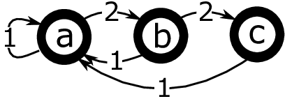
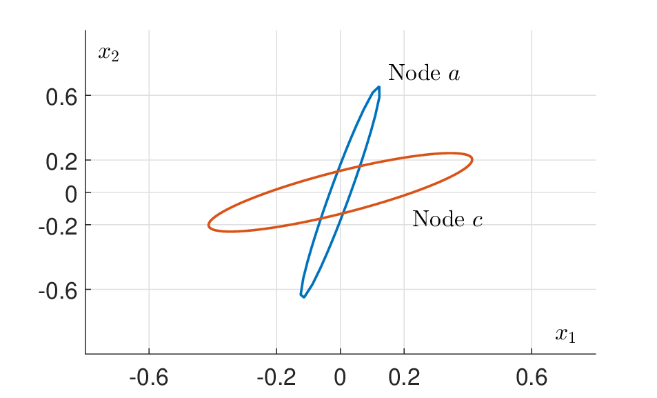
The system here is actually not minimal. Indeed, take the third node . Any vector of the form satisfies , for any such that . Thus, . From there, we can see that at nodes and , and are formed of any vector of the form , where . Thus, . Applying Theorem II.7 to the system (after applying Remark 1), we obtain a minimal rectangular system with nodal dimensions . We can then approximate the storage functions . Applying Proposition III.1 with paths of length 10, we obtain, a lower-bound on the gain
We use this bound to compute the approximations of , . The level sets of these functions are displayed on Figure 3.

V Conclusion.
We provide a general characterization of the -gain of discrete-time linear switching system under the form of switching storage functions. Under the assumptions of internal stability and minimality, the pieces of these functions are the th power of norms. The generality of these assumptions is discussed and we provide means to compute minimal realizations of constrained switching systems. We then turn our focus on the gain, and provide algorithms for obtaining asymptotically tight lower and upper bounds on the gain based on the approximation of storage functions. Finally, we provide a converse result for the existence of quadratic storage functions exploiting the nature of storage functions, and formulate a conjecture about Horizon-Dependent storage functions. We believe an answer to the conjecture (positive or negative) will allow for a better understanding of the geometry underlying Lyapunov methods for performance analysis.
References
- [1] A. A. Ahmadi, R. M. Jungers, P. A. Parrilo, and M. Roozbehani, “Joint spectral radius and path-complete graph lyapunov functions,” SIAM Journal on Control and Optimization, vol. 52, no. 1, pp. 687–717, 2014.
- [2] R. Alur, A. D’Innocenzo, K. H. Johansson, G. J. Pappas, and G. Weiss, “Compositional modeling and analysis of multi-hop control networks,” IEEE Transactions on Automatic control, vol. 56, no. 10, pp. 2345–2357, 2011.
- [3] T. Ando and M.-H. Shih, “Simultaneous contractibility,” SIAM Journal on Matrix Analysis and Applications, 19(2), 487-498, 1998.
- [4] P.-A. Bliman and G. Ferrari-Trecate, “Stability analysis of discrete-time switched systems through lyapunov functions with nonminimal state,” in Proceedings of IFAC Conference on the Analysis and Design of Hybrid Systems, 2003, pp. 325–330.
- [5] V. D. Blondel, Y. Nesterov, and J. Theys, “On the accuracy of the ellipsoid norm approximation of the joint spectral radius,” Linear Algebra and its Applications, vol. 394, pp. 91–107, 2005.
- [6] V. D. Blondel and J. N. Tsitsiklis, “The boundedness of all products of a pair of matrices is undecidable,” Systems & Control Letters, vol. 41, no. 2, pp. 135–140, 2000.
- [7] P. Colaneri, P. Bolzern, and J. C. Geromel, “Root mean square gain of discrete-time switched linear systems under dwell time constraints,” Automatica, vol. 47, no. 8, pp. 1677–1684, 2011.
- [8] J. Daafouz and J. Bernussou, “Parameter dependent lyapunov functions for discrete time systems with time varying parametric uncertainties,” Systems & Control Letters, vol. 43, no. 5, pp. 355–359, 2001.
- [9] X. Dai, “A Gel’fand-type spectral radius formula and stability of linear constrained switching systems,” Linear Algebra and its Applications, vol. 436, no. 5, pp. 1099–1113, 2012.
- [10] G. E. Dullerud and S. Lall, “A new approach for analysis and synthesis of time-varying systems,” IEEE Transactions on Automatic Control, vol. 44, no. 8, pp. 1486–1497, 1999.
- [11] R. Essick, J.-W. Lee, and G. E. Dullerud, “Control of linear switched systems with receding horizon modal information,” IEEE Transactions on Automatic Control, vol. 59, no. 9, pp. 2340–2352, 2014.
- [12] R. Essick, M. Philippe, G. Dullerud, and R. M. Jungers, “The minimum achievable stability radius of switched linear systems with feedback,” in IEEE 54th Annual Conference on Decision and Control (CDC). IEEE, 2015, pp. 4240–4245.
- [13] E. A. Hernandez-Vargas, R. H. Middleton, and P. Colaneri, “Optimal and mpc switching strategies for mitigating viral mutation and escape,” in Proc. of the 18th IFAC World Congress Milano (Italy) August, 2011.
- [14] J. P. Hespanha, “L2-induced gains of switched linear systems,” Unsolved problems in mathematical systems and control theory, p. 131, 2004.
- [15] K. Hirata and J. P. Hespanha, “L2-induced gain analysis of switched linear systems via finitely parametrized storage functions,” in American Control Conference (ACC), 2010. IEEE, 2010, pp. 4064–4069.
- [16] R. Jungers, “The joint spectral radius,” Lecture Notes in Control and Information Sciences, vol. 385, 2009.
- [17] R. M. Jungers, A. D’Innocenzo, and M. D. Di Benedetto, “Feedback stabilization of dynamical systems with switched delays,” in Proc. of the 51st IEEE Conference on Decision and Control, 2012, pp. 1325–1330.
- [18] V. Kozyakin, “The Berger–Wang formula for the markovian joint spectral radius,” Linear Algebra and its Applications, vol. 448, pp. 315–328, 2014.
- [19] A. Kundu and D. Chatterjee, “Stabilizing switching signals for switched systems,” IEEE Transactions on Automatic Control,, vol. 60, no. 3, pp. 882–888, 2015.
- [20] J.-W. Lee and G. E. Dullerud, “Optimal disturbance attenuation for discrete-time switched and markovian jump linear systems,” SIAM Journal on Control and Optimization, vol. 45, no. 4, pp. 1329–1358, 2006.
- [21] ——, “Uniform stabilization of discrete-time switched and markovian jump linear systems,” Automatica, 42(2), 205-218, 2006.
- [22] D. Liberzon, Switching in systems and control. Springer Science & Business Media, 2012.
- [23] D. Liberzon and A. S. Morse, “Basic problems in stability and design of switched systems,” IEEE Control Systems Magazine, vol. 19, no. 5, pp. 59–70, 1999.
- [24] M. Naghnaeian and P. Voulgaris, “Characterization and optimization of l1 gains of linear switched systems.”
- [25] M. Naghnaeian, P. G. Voulgaris, and G. E. Dullerud, “A unified framework for lp analysis and synthesis of linear switched systems,” in 2016 American Control Conference (ACC). IEEE, 2016, pp. 715–720.
- [26] M. Petreczky, L. Bako, and J. H. Van Schuppen, “Realization theory of discrete-time linear switched systems,” Automatica, vol. 49, no. 11, pp. 3337–3344, 2013.
- [27] M. Petreczky and J. H. van Schuppen, “Realization theory of discrete-time linear hybrid system,” IFAC Proceedings Volumes, vol. 42, no. 10, pp. 593–598, 2009.
- [28] M. Philippe, R. Essick, G. Dullerud, and R. M. Jungers, “Stability of discrete-time switching systems with constrained switching sequences,” Automatica, vol. 72, pp. 242–250, 2016.
- [29] M. Philippe, G. Millerioux, and R. M. Jungers, “Deciding the boundedness and dead-beat stability of constrained switching systems,” Nonlinear Analysis: Hybrid Systems, 2016.
- [30] V. Putta, G. Zhu, J. Shen, and J. Hu, “A study of the generalized input-to-state l2-gain of discrete-time switched linear systems,” in 50th IEEE Conference on Decision and Control and European Control Conference, 2011, pp. 435–440.
- [31] R. Shorten, F. Wirth, and D. Leith, “A positive systems model of tcp-like congestion control: asymptotic results,” IEEE/ACM Transactions on Networking, vol. 14, no. 3, pp. 616–629, 2006.