Spatiotemporal Stochastic Modeling of IoT Enabled Cellular Networks: Scalability and Stability AnalysisThanks:  The authors are with the Electrical Engineering Program, Computer, Electrical, and Mathematical Sciences and Engineering (CEMSE) Division, King Abdullah University of Science and Technology (KAUST), Thuwal, Saudi Arabia; e-mails: {mohammad.gharbieh, hesham.elsawy, ahmed.bader, slim.alouini}@kaust.edu.sa.

While the queue arrival process is a function of the underlying IoT application only, the queue departure (i.e., service) process depends on the transmission signal-to-interference-plus-noise ratio (SINR) across time slots. We first show that the SINR involves a negligible temporal correlation across time slots due to the interference temporal correlation. Therefore, we drop the time index and assume independent SINR at each time slot. Then, we employ a two-dimensional Geo/PH/1 DTMC for each IoT device, where Geo stands for geometric inter-arrival process and PH stands for the Phase-type departure process [20, 21]. The Geo/PH/1 queueing model is particularly chosen for its simplified memoryless inter-arrival process and its general departure process that can account for the interference based interactions between the IoT queues. To this end, we study three different transmission protocols that are defined by cellular systems for uplink random channel access [22], namely, the baseline scheme, the power-ramping scheme, and backoff scheme. For each protocol, we derive sufficient conditions and necessary conditions for network stability, in which the stability is defined according to Loynes theorem [23]. That is, the network is considered stable if the average arrival rate is less than the average service rate for a randomly selected queue in the network. The scalability and stability tradeoff in IoT cellular networks is then determined by plotting the Pareto-frontier of the stability region defined by the arrival process, the intensity of IoT devices, and the SINR detection threshold. The Pareto-frontier of the stability region shows the spatial traffic intensity limit (i.e., the maximum limit of IoT density for a given traffic requirement) that a cellular network can support, beyond which the queues become unstable and packets are lost with probability one. For stable networks, we obtain the average queue size, the average packet delay, and the average service time. On the other hand, for unstable networks, we only calculate the average service time. The contributions of this paper can be summarized by the following:

• •

  Develop a novel spatiotemporal mathematical paradigm for IoT enabled cellular networks.

• •

  Integrate two dimensional Geo/PH/1 DTMC within stochastic geometry framework to account for interference based queue interactions in large-scale IoT network.

• •

  Derive sufficient and necessary conditions for IoT network stability.

• •

  Characterize the scalability/stability tradeoff by showing the maximum spatial traffic intensity that a cellular network can accommodate.

• •

  Assess and compare three different transmission schemes in terms of transmission success probability, average packet delay, and average queue size.

The rest of the paper is organized as follows. Section II presents the system model and the assumptions. The outline of the analytical framework is established in Section III. Section IV characterizes the different transmission schemes. Section V provides the numerical and simulation results. Finally, Section VI concludes the paper.

We consider an IoT-enabled cellular network in which the cellular BSs and the IoT devices are spatially distributed in $\mathbb{R}^{2}$ according to two independent homogeneous PPPs, denoted as $\Psi$ and $\Phi$, with intensities $\lambda$ and $\mathcal{U}$, respectively. Without loss of generality, each of the devices is assumed to communicate its packets via the nearest BS. The average number of devices connected to each BS is $\alpha=\frac{\mathcal{U}}{\lambda}$.

A power-law path-loss model is considered where the signal power decays at a rate $r^{-\eta}$ with the propagation distance $r$, where $\eta>2$ is the path-loss exponent. In addition to the path-loss attenuation, Rayleigh fading multipath environment is assumed where the intended and interfering channel power gains ($h$ and $g$) are exponentially distributed with unity mean. All channel gains are assumed to be independent of each other, independent of the spatial locations, and are identically distributed (i.i.d). The IoT devices use full path-loss inversion power control with a threshold $\rho$. That is, each device controls its transmit power such that the average signal power received at the serving BS is equal to a predefined value $\rho$, which is assumed to be the same for all the BSs. It is assumed that the BSs are dense enough such that each of the devices can invert its path loss towards the closest BS almost surely, and hence the maximum transmit power of the IoT devices is not a binding constraint for packet transmission. Since the main focus of this paper is to integrate stochastic geometry and DTMCs to study scalability and stability of IoT enabled cellular networks, we particularly select power-law path-loss, Rayleigh fading, and full-path-loss inversion for mathematical simplicity. Future extensions of this work may include multi-slope path loss models [24, 25], advanced fading models [26], multi-antenna [27], and/or fractional channel inversion power control [27, 28].

This paper considers a synchronous time slotted cellular system and geometric packet inter-arrival process with parameter $a\in[0,1]$ (packet/slot) at each IoT device. We assume that the duration of each time slot is small enough such that a single packet arrival and/or departure can take place per time slot. The arrived packets at each IoT device are stored in a buffer (i.e., queue) with infinite length until successful transmission.²² 2 The infinite buffer is assumed for mathematical convenience. In Section V, it is shown that small buffer sizes are sufficient as long as the network is stable. Otherwise, the buffers of the devices will overflow irrespective of their sizes. The BSs are unaware about the queue status of the devices, and hence, no scheduling decision for the packets is taken at the BS side. Therefore, we assume that each device with non-empty queue directly transmits backlogged packets via a First Come First Served (FCFS) service discipline, which complies with the narrow-band IoT (NB-IoT) operation defined by the 3GPP standard [2].

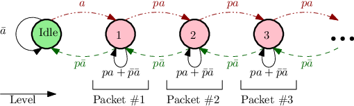
A two-dimensional Geo/PH/1 Markov chain is employed to model each IoT device, in which the levels indicate the number of packets in the queue and the phases indicate the transmission protocol states. Let $p_{m}$ be the probability of packet transmission success when the IoT device operate at transmission phase $m$ and let $(\bar{\cdot})=(1-\cdot)$ denote the probability complement operator. Then, the considered transmission protocols are shown in Figs. 1, 2(a), and 2(b), which are described below:

From the queueing perspective, the PH type distribution tracks the phases that the queue may experience until the packet is successfully transmitted. Let $n$ be the number of transient phases. Following [21], the PH type distribution is defined by the tuple ($\boldsymbol{\beta},\mathbf{S}$), where $\mathbf{S}\in\mathbb{R}^{n\times n}$ is the transient sub-stochastic matrix and $\boldsymbol{\beta}\in\mathbb{R}^{1\times n}$ is the initialization row-vector for the transient states. Particularly, the PH type distribution models the service procedure with an absorbing Markov chain with the following transition matrix

where $\mathbf{s}\in\mathbb{R}^{n\times 1}$ is given by $\mathbf{s}=\mathbf{e}-\mathbf{S}\times\mathbf{e}$ and $\mathbf{e}$ is a column vector of ones with the proper length. From (1), it is clear that $\mathbf{S}$ captures the transition probabilities between phases until absorption and $\mathbf{s}$ captures the probability of absorption from each phase, in which absorption corresponds to successful packet transmission through the channel. Exploiting the MAM with PH type service along with the packet-by-packet generation and service assumption, each IoT device employing any of the aforementioned transmission schemes can be represented by a Quasi-Birth-Death (QBD) queueing model with the following general probability transition matrix

where $B\in\mathbb{R},\mathbb{C}\in\mathbb{R}^{1\times n},\mathbb{E}\in\mathbb{R}^{n\times 1},\mathbb{A}_{0}\in\mathbb{R}^{n\times n},\mathbb{A}_{1}\in\mathbb{R}^{n\times n}$, and $\mathbb{A}_{2}\in\mathbb{R}^{n\times n}$ are the sub-stochastic matrices that capture the transitions between the queue levels. Particularly, the sub-matrix $\mathbb{A}_{0}=a\mathbf{S}$ captures the event where a packet arrives while being in the transient service state, which increases the number of packets in the queue by one. The sub-matrix $\mathbb{A}_{2}=\bar{a}\mathbf{s}\boldsymbol{\beta}$ captures the event where a service completion occurs and no packet arrives, which decreases the number of packets in the queue by one. The sub-matrix $\mathbb{A}_{1}=a\mathbf{s}\boldsymbol{\beta}+\bar{a}\mathbf{S}$ captures the events where a service completion occurs and a packet arrives or no packet arrives while being in transient state, which leaves the number of packets in the queue unchanged. The transitions captured by $\mathbb{A}_{2}$, $\mathbb{A}_{1}$, and $\mathbb{A}_{0}$ are visualized in Figs. 1, 2(a), and 2(b) by green, red, and black arrows, respectively. Boundary vectors $B=\bar{a},\mathbb{C}=a\boldsymbol{\beta}$, and $\mathbb{E}=\bar{a}\mathbf{s}$ capture the transitions from idle-to-idle, idle-to-level (i=1), and from level (i=1)-to-idle, respectively. Note that $B,\mathbb{C}$, and $\mathbb{E}$ have different sizes than $\mathbb{A}_{2}$, $\mathbb{A}_{1}$, and $\mathbb{A}_{0}$ due to the different phase structure between the idle state and the other levels $(i\geq 1)$. It is worth noting that the vector $\boldsymbol{\beta}$ appears in $\mathbb{C},\mathbb{A}_{1},$ and $\mathbb{A}_{2}$ to initialize the transient service states for a new packet.

Let $\mathbb{A}=\mathbb{A}_{0}+\mathbb{A}_{1}+\mathbb{A}_{2}$, and let the vector $\boldsymbol{\pi}$ be the unique solution of $\boldsymbol{\pi}\mathbb{A}=\boldsymbol{\pi}$ with the normalization condition $\boldsymbol{\pi}\mathbf{e}=1$. Then, the DTMC in (2) is stable if and only if $\boldsymbol{\pi}\mathbb{A}_{2}\mathbf{e}>\boldsymbol{\pi}\mathbb{A}_{0}\mathbf{e}$, which implies that the departure rate is higher that the arrival rate [21, 20]. For stable systems, the steady state solution can be obtained by solving

where $\mathbf{x}=[x_{\circ},x_{1,1}x_{1,2},\dots,x_{i,j-1},x_{i,j},x_{i,j+1}\dots]$ is the row vector that contains the steady-state probabilities, in which $x_{\circ}$ denotes the idle state probability and $x_{i,j}$ is the probability of being in level $i$ and phase $j$. Note that $\mathbf{x}$ is also denoted as the steady state distribution of the queue. When the stability condition ($\boldsymbol{\pi}\mathbb{A}_{2}\mathbf{e}>\boldsymbol{\pi}\mathbb{A}_{0}\mathbf{e}$) is not satisfied, the queue becomes unstable and the queue length grows indefinitely and the system in (3) with the transissiom matrix in (2) cannot be analyzed [20, 21]. Consequently, we abstract the queue size for unstable queues and look into the marginal phase distribution only $\mathbb{\Pi}$ as shown in Figs. 3(a) and 3(b), which is obtained by solving the following system

such that $\boldsymbol{\Pi}$ contains the probabilities for the states shown in Figs. 3(a) and 3(b). Note that these systems are finite and ergodic, and hence, are always stable.

To analyze the queue stability and solve the above queueing systems, the PH type distribution parameters ($\boldsymbol{\beta},\mathbf{S}$) should be determined. As discussed earlier and shown in Figs. 1, 2(a), and 2(b), the transmission protocol restarts its phases after each successful transmission. Hence, $\boldsymbol{\beta}\!\!=\!\!\{1,\boldsymbol{0}\}$ where $\boldsymbol{0}$ is a row vector of zeros with the proper length. This makes $\mathbf{S}$ the only missing component to solve the presented queueing model. Figs. 1 and 2 show that $\mathbf{S}$ involve computing the transmission probabilities $p$ and $p_{m}$, which are discussed in the next section.

A packet sent by an IoT device (i.e., queue) is successfully decoded at the serving BS (i.e., server) if the SINR at the BS exceeds a certain threshold $\theta$. Mathematically, the transmission success probabilities for the baseline and backoff schemes are expressed as

where $\tilde{\Phi}_{k}$ is the set containing the locations of interfering devices operating with power control $\rho_{k}$, $P_{i,k}$ is the transmit power of the $i^{th}$ device in $\tilde{\Phi}_{k}$, $\mathcal{I}_{k}$ is the aggregate interference power from devices in $\tilde{\Phi}_{k}$. The transmit powers $P_{i}$ and $P_{i,k}$ in (5) and (6) are random variables that depend on the distance between the i^th interfering IoT device and its own serving BS. The expression in (6) follows from the employed channel inversion power control, the exponential distribution of $h_{\circ}$, the definition of the Laplace transform, and the independence between $\tilde{\Phi}_{k}$, $\forall k$ at a given time slot. Equations (5) and (6) capture the interactions between the queues in the aggregate interference term. The equations also involve the effect of propagation, fading, and power control on the transmission success probabilities. The interference terms in (5) and (6) are functions of the points processes $\tilde{\Phi}$ and $\tilde{\Phi}_{k}$, respectively. Due to the random pseudo code selection and the independent thinning property of the PPP, both $\tilde{\Phi}$ and $\tilde{\Phi}_{k}$ are PPPs at any time slot. However, there may exist common interfering devices seen by the same BS from one time slot to another, which introduces temporal correlation for the success probability. Such temporal correlation involves memory to the queues and highly complicates the queueing analysis. Furthermore, the transmission powers of nearby devices are spatially correlated due to the employed channel inversion power control. Such temporal and spatial correlations impede the model tractability. Fortunately, the aforementioned temporal and spatial correlations have a negligible impact on the performance of the employed system model, which is verified by numerical results and simulations. Formal statements and comments on the involved approximations are given in the sequel.

The queueing and stochastic geometry analysis discussed in Sections III-A and III-B are interdependent, which impose a causality problem. Particularly, the matrix $\mathbf{S}$ that is required to construct and solve the queuing model in Section III-A depends on the transmission success probabilities in (5) and (6) of Section III-B. The converse is also true, the point processes $\tilde{\Phi}$ and $\tilde{\Phi}_{n}$ in (5) and (6) of Section III-B are constructed based on the steady state solution of (3) in Section III-A. To solve this causality problem, we employ the iterative solution, shown in Algorithm 1, to find the steady state probabilities and the associated aggregate interference.

The iterative algorithm in Algorithm 1 is equivalent to solving the system

where $\mathbf{P}\!\!\left(\mathbf{x}^{[i-1]}\right)$ is updated based on (5) and (6). Due to the ergodicity of the used queueing models, the system in (7) has a unique solution $\mathbf{x}^{[i]}$ for each $\mathbf{x}^{[i-1]}$ [21]. Hence, the Algorithm 1 converges by virtue of the fixed point theorem [38].

After determining the steady state solution $\mathbf{x}$ for the system via Algorithm 1, many performance metrics can be obtained. For instance, transmission success probability at steady state is

For stable systems, we can additionally find the average queue size, denoted as $\mathbb{E}[Q_{L}]$, and the average queueing delay, denoted as $\mathbb{E}[W_{q}]$. Let $Q_{L}$ be instantaneous queue size, then the average queue size in given by

where,

We start by the baseline scheme, which is the simplest transmission scheme. Fig. 1 shows that the baseline scheme has only one transmission phase. Hence, the transient state of (1) is just $\textbf{S}=\bar{p}$, where $p$ is the transmission success probability given by (5). This reduces the Geo/PH/1 queueing model in (2) to a simple Geo/Geo/1 queue with the following transmission matrix

Let $\mathbf{x}=[x_{\circ},\ x_{1},\ x_{2},\ \ldots,\ ]$ be the stationary distribution, where $x_{i}$ represents the probability of having $i$ packets in the queue, then solving (3) with the transition matrix in (13) gives

Using stochastic geometry, the transmission success probability $p$ for the baseline scheme is characterized via the following lemma.

In the power-ramping scheme, the transmission success probability depends on the transmission phase, and hence, a Geo/PH/1 queueing model is employed. From Fig. 2(a), it can be observed that each IoT device increments its power control threshold upon transmission failure, which gives the following PH type transient matrix

Let $\mathbf{x}=[x_{\circ},\mathbb{x}_{1},\mathbb{x}_{2},\ \ldots,\ ]$ be the stationary distribution, where $x_{\circ}$ represents the probability of having an idle queue and $\mathbb{x}_{i}=[x_{i,1}x_{i,2}\dots x_{i,M}]$ is the probability vector for transmission phases when of having $i$ packets in the queue. The steady state solution for the power-ramping queueing model is given in the following lemma

In the backoff scheme, the IoT devices defer their transmissions and go to backoff upon transmission failures. From Fig. 2(a), it can be observed that there are deterministic and probabilistic backoff states in which the PH type transient matrix can be represented as

Let $\mathbf{x}=[x_{\circ},x_{1,1},x_{1,2},\dots,x_{i,j-1},x_{i,j},x_{i,j+1}\dots]$ be the stationary distribution, where $x_{\circ}$ represents the probability of having an idle queue, $x_{i,1}$ represents the probability of being in the transmission phase, and $x_{i,j}$ for $i\geq 1$ and $j>1$ represents the probability of being in one of the backoff phases (i.e., having non-empty buffer but not transmitting). The steady state solution for the backoff scheme can be obtained via Lemma 3 but with $\mathbb{S}$ given in (29).

Using the same definition for $\mathbb{\Pi}$ as in Section IV-B, it is noticed that $\Pi_{1}$ is the probability of being in transmission state and $\Pi_{n}$ $n>1$ is the probability of being in the backoff phase. The marginal distribution $\mathbb{\Pi}$ for the backoff scheme can be obtained via (22) but with $\mathbb{S}$ given in (29). As discussed earlier, the marginal distribution $\mathbb{\Pi}$ is required to obtain the transmission success probability, which is given in the following lemma.

References

- [1] A. Al-Fuqaha, M. Guizani, M. Mohammadi, M. Aledhari, and M. Ayyash, “Internet of things: A survey on enabling technologies, protocols, and applications,” IEEE Commun. Surveys Tuts., vol. 17, no. 4, pp. 2347–2376, Fourthquarter 2015.
- [2] Ericsson Technology Review, “NB-IoT: A sustainable technology for connecting billions of devices,” vol. 93, no. 2, 2016. [Online]. Available: https://www.ericsson.com/thecompany/our_publications/ericsson_technology_review
- [3] K. Zheng, F. Hu, W. Wang, W. Xiang, and M. Dohler, “Radio resource allocation in LTE-advanced cellular networks with M2M communications,” IEEE Commun. Mag., vol. 50, no. 7, pp. 184–192, July 2012.
- [4] M. R. Palattella, M. Dohler, A. Grieco, G. Rizzo, J. Torsner, T. Engel, and L. Ladid, “Internet of things in the 5G era: Enablers, architecture, and business models,” IEEE J. Sel. Areas Commun., vol. 34, no. 3, pp. 510–527, March 2016.
- [5] M. Gerasimenko, V. Petrov, O. Galinina, S. Andreev, and Y. Koucheryavy, “Energy and delay analysis of LTE-advanced RACH performance under MTC overload,” in IEEE Global Communications Conference (GLOBECOM) Workshops, Anaheim, USA, Dec 2012, pp. 1632–1637.
- [6] M. Polese, M. Centenaro, A. Zanella, and M. Zorzi, “On the evaluation of LTE random access channel overload in a smart city scenario,” in Proc. of the 2016 IEEE International Conference on Communications (ICC), Kuala Lumpur , Malaysia, May 2016.
- [7] A. Bader, H. ElSawy, M. Gharbieh, M.-S. Alouini, A. Adinoyi, and F. Alshaalan, “First mile challenges for large-scale IoT,” IEEE Commun. Mag., March 2017.
- [8] R. R. Rao and A. Ephremides, “On the stability of interacting queues in a multiple-access system,” IEEE Trans. Inf. Theory, vol. 34, no. 5, pp. 918–930, Sep 1988.
- [9] V. Anantharam, “The stability region of the finite-user slotted ALOHA protocol,” in Decision and Control, 1989., Proceedings of the 28th IEEE Conference on, Dec 1989, pp. 579–584 vol.1.
- [10] W. Luo and A. Ephremides, “Stability of N interacting queues in random-access systems,” IEEE Trans. Inf. Theory, vol. 45, no. 5, pp. 1579–1587, Jul 1999.
- [11] N. Xie, J. M. Walsh, and S. Weber, “Properties of an ALOHA-like stability region,” arXiv preprint arXiv:1408.3469, 2014.
- [12] M. Haenggi, Stochastic Geometry for Wireless Networks. Cambridge University Press, 2012.
- [13] H. ElSawy, E. Hossain, and M. Haenggi, “Stochastic geometry for modeling, analysis, and design of multi-tier and cognitive cellular wireless networks: A survey,” IEEE Commun. Surveys Tuts., vol. 15, no. 3, pp. 996–1019, 2013.
- [14] H. ElSawy, A. Sultan-Salem, M.-S. Alouini, and M. Z. Win, “Modeling and analysis of cellular networks using stochastic geometry: A tutorial,” IEEE Commun. Surveys Tuts., to appear 2017.
- [15] Y. Zhong, M. Haenggi, T. Q. S. Quek, and W. Zhang, “On the stability of static poisson networks under random access,” IEEE Trans. Commun., accepted 2016.
- [16] M. Gharbieh, H. ElSawy, A. Bader, and M. S. Alouini, “Tractable stochastic geometry model for iot access in lte networks,” in 2016 IEEE Global Communications Conference (GLOBECOM), Dec 2016, pp. 1–7.
- [17] J. G. Andrews, F. Baccelli, and R. K. Ganti, “A tractable approach to coverage and rate in cellular networks,” IEEE Trans. Commun., vol. 59, no. 11, pp. 3122–3134, 2011.
- [18] A. Guo and M. Haenggi, “Spatial stochastic models and metrics for the structure of base stations in cellular networks,” IEEE Trans. Wireless Commun., vol. 12, no. 11, pp. 5800–5812, Nov. 2013.
- [19] W. Lu and M. D. Renzo, “Stochastic geometry modeling of cellular networks: Analysis, simulation and experimental validation,” CoRR, vol. abs/1506.03857, 2015. [Online]. Available: http://arxiv.org/abs/1506.03857
- [20] G. Latouche and V. Ramaswami, Introduction to matrix analytic methods in stochastic modeling. Siam, 1999, vol. 5.
- [21] A. S. Alfa, Applied Discrete-Time Queues. Springer New York, 2015.
- [22] S. Sesia, I. Toufik, and M. Baker, LTE: the UMTS long term evolution. Wiley Online Library, 2009.
- [23] R. Loyens, “The stability of a queue with non-independent inter-arrival and service times,” in Proc. Cambridge Philos. Soc, vol. 58, no. 3, pp. 470–520, 1962.
- [24] M. D. Renzo, W. Lu, and P. Guan, “The intensity matching approach: A tractable stochastic geometry approximation to system-level analysis of cellular networks,” IEEE Trans. Wireless Commun., vol. 15, no. 9, pp. 5963–5983, Sept 2016.
- [25] J. G. Andrews, X. Zhang, G. D. Durgin, and A. K. Gupta, “Are we approaching the fundamental limits of wireless network densification?” IEEE Commun. Mag., vol. 54, no. 10, pp. 184–190, October 2016.
- [26] A. AlAmmouri, H. ElSawy, A. Sultan-Salem, M. D. Renzo, and M. S. Alouini, “Modeling cellular networks in fading environments with dominant specular components,” in 2016 IEEE International Conference on Communications (ICC), May 2016, pp. 1–7.
- [27] M. D. Renzo and P. Guan, “Stochastic geometry modeling and system-level analysis of uplink heterogeneous cellular networks with multi-antenna base stations,” IEEE Trans. Commun., vol. 64, no. 6, pp. 2453–2476, June 2016.
- [28] S. Singh, X. Zhang, and J. G. Andrews, “Joint rate and SINR coverage analysis for decoupled uplink-downlink biased cell associations in HetNets,” IEEE Trans. Wireless Commun., vol. 14, no. 10, pp. 5360–5373, Oct 2015.
- [29] H. ElSawy and E. Hossain, “On stochastic geometry modeling of cellular uplink transmission with truncated channel inversion power control,” IEEE Trans. Wireless Commun., vol. 13, no. 8, pp. 4454–4469, 2014.
- [30] T. D. Novlan, H. S. Dhillon, and J. G. Andrews, “Analytical modeling of uplink cellular networks,” IEEE Trans. Wireless Commun., vol. 12, no. 6, pp. 2669–2679, June 2013.
- [31] H. Y. Lee, Y. J. Sang, and K. S. Kim, “On the uplink sir distributions in heterogeneous cellular networks,” IEEE Commun. Lett., vol. 18, no. 12, pp. 2145–2148, Dec 2014.
- [32] F. J. Martin-Vega, G. Gomez, M. C. Aguayo-Torres, and M. D. Renzo, “Analytical modeling of interference aware power control for the uplink of heterogeneous cellular networks,” IEEE Trans. Wireless Commun., vol. 15, no. 10, pp. 6742–6757, Oct 2016.
- [33] Y. Zhong, W. Zhang, and M. Haenggi, “Managing interference correlation through random medium access,” IEEE Trans. Wireless Commun., vol. 13, no. 2, pp. 928–941, February 2014.
- [34] S. Singh, H. S. Dhillon, and J. G. Andrews, “Offloading in heterogeneous networks: Modeling, analysis, and design insights,” IEEE Trans. Wireless Commun., vol. 12, no. 5, pp. 2484–2497, May 2013.
- [35] H. ElSawy, E. Hossain, and S. Camorlinga, “Traffic offloading techniques in two-tier femtocell networks,” in 2013 IEEE International Conference on Communications (ICC), June 2013, pp. 6086–6090.
- [36] A. AlAmmouri, H. ElSawy, and M.-S. Alouini, “Load-aware modeling for uplink cellular networks in a multi-channel environment,” in Proc. of the 25th IEEE Personal Indoor and Mobile Radio Communications (PIMRC’14), Washington D.C., USA, Sep. 2014.
- [37] H. S. Dhillon and J. G. Andrews, “Downlink rate distribution in heterogeneous cellular networks under generalized cell selection,” IEEE Wireless Commun. Lett., vol. 3, no. 1, pp. 42–45, February 2014.
- [38] L. Sartori, S. E. Elayoubi, B. Fourestie, and Z. Nouir, “On the WiMAX and HSDPA coexistence,” in 2007 IEEE International Conference on Communications, June 2007, pp. 5636–5641.
- [39] G. Nigam, P. Minero, and M. Haenggi, “Spatiotemporal cooperation in heterogeneous cellular networks,” IEEE J. Sel. Areas Commun., vol. 33, no. 6, pp. 1253–1265, June 2015.
- [40] H. ElSawy and E. Hossain, “On cognitive small cells in two-tier heterogeneous networks,” in 11th International Symposium on Modeling Optimization in Mobile, Ad Hoc Wireless Networks (WiOpt), May 2013, pp. 75–82.