Hermite interpolation by piecewise polynomial surfaces with polynomial area element
Abstract
This paper is devoted to the construction of polynomial 2-surfaces which possess a polynomial area element. In particular we study these surfaces in the Euclidean space (where they are equivalent to the PN surfaces) and in the Minkowski space (where they provide the MOS surfaces). We show generally in real vector spaces of any dimension and any metric that the Gram determinant of a parametric set of subspaces is a perfect square if and only if the Gram determinant of its orthogonal complement is a perfect square. Consequently the polynomial surfaces of a given degree with polynomial area element can be constructed from the prescribed normal fields solving a system of linear equations. The degree of the constructed surface depending on the degree and the quality of the prescribed normal field is investigated and discussed. We use the presented approach to interpolate a network of points and associated normals with piecewise polynomial surfaces with polynomial area element and demonstrate our method on a number of examples (constructions of quadrilateral as well as triangular patches).
Keywords:
Hermite interpolation , PN surfaces , MOS surfaces , polynomial area element1 Introduction
Rational surfaces with Pythagorean normal vector fields (PN surfaces) were introduced by Pottmann (1995) as a surface analogy to Pythagorean hodograph (PH) curves defined previously by Farouki and Sakkalis (1990). For a survey of shapes with Pythagorean property see e.g. (Farouki, 2008) and references therein. It holds that PH curves in plane and PN surfaces in space considered as hypersurfaces share some common properties, e.g. they both yield rational offsets. Nevertheless there exist lot of significant differences between these classes of rational varieties. For instance, the curves with Pythagorean hodographs were introduced as planar polynomial shapes and a compact formula for their description based on Pythagorean triples of polynomials is available. On the other hand, a description of rational Pythagorean normal vector surfaces reflecting their dual description was revealed first in (Pottmann, 1995) and it is still not known how to specify these formulas to obtain from them the subclass of polynomial PN surfaces. This could be probably one of the reasons why the PN surfaces do not have as many particular applications as the PH curves. Nonetheless, new attempts to study PN surfaces has again begun recently, see (Kozak et al., 2016; Lávička et al., 2016).
Indeed, when working with PH curves and PN surfaces then focusing only on the rationality of their offsets can conceal other important properties and it does not offer a full overview of their useful features. In the curve case, another (or maybe the main) very important practical application is based on the fact that the parametric speed (or the length element), and thus also the arc length, of polynomial PH curves is polynomial, too. This is important for formulating efficient real time interpolator algorithms for CNC machines. We recall that the interpolators for general NURBS curves are typically computed using Taylor series expansions. Of course, this approach brings truncation errors caused by omitting higher-order terms. When the Pythagorean hodograph curves are applied for describing the tool path, this problem is overcome. The concept of planar polynomial PH curves was generalized also to spatial polynomial PH curves (Farouki and Sakkalis, 1994) which are not hypersurfaces anymore and thus we do not construct their offsets as in the plane case. This can be taken as another reason for preferring the polynomiality of the parametric speed over the rationality of their offsets as a main distinguishing property. Later, planar and spatial PH curves were studied also as rational objects (Pottmann, 1995; Farouki and Šír, 2011). However, we would like to emphasize that for rational PH curves their arc length does not have to be expressible as a rational function of the parameter as the integral of a rational function is not rational, in general.
Analogously to the parametric speed and the arc length in the curve case we recall the area element and the surface area for surfaces. Clearly, the area element, and thus also the surface area, of polynomial PN surfaces is polynomial but the surface area of rational PN surfaces is again not rational, in general. This underlines a prominent role of polynomial PN surfaces and shows a more natural relation between polynomial PH curves to polynomial PN surfaces rather then the rationality of their offsets. Moreover, as the curves with the polynomial/rational line element (i.e., PH curves) can be defined in any arbitrary dimension, the same holds also for the surfaces with the polynomial/rational area element, whose special instances the PN surfaces in 3-space are. Unfortunately, there is not known very much about polynomial PN surfaces. As a particular result we can mention the investigation of a remarkable family of cubic polynomial PN surfaces with birational Gauss mapping, which represent a surface counterpart to the planar Tschirnhausen cubic, the simplest planar polynomial PH curve. A full description of these PN surfaces, among which e.g. the Enneper surface belongs, was presented and their properties were thoroughly discussed in Lávička and Vršek (2012). Recently an approach for a construction of polynomial PN surfaces based on bivariate polynomials with quaternion coefficients was presented by Kozak et al. (2016).
As concerns modelling techniques formulated for PN surfaces, in particular the Hermite interpolation schemes by piecewise PN surfaces, there are not many results from this area. One can find a few indirect algorithms for the interpolations with PN surfaces, where ‘indirect’ means that the resulting surfaces become rational PN only after a suitable reparameterization – we recall e.g. (Jüttler and Sampoli, 2000; Bastl et al., 2008); however these must be always followed by non-trivial trimming of the parameter domain. One can find also a few direct algorithms based on the dual approach, which is especially convenient for PN surfaces, see e.g. (Peternell and Pottmann, 1996; Lávička et al., 2016). Nevertheless these approaches produce rational PN surfaces and are inapplicable when polynomial parameterizations are required. As far as we are aware, the algorithm presented in this paper is the first functional and complex method solving the Hermite problem directly (i.e., without a need of any consequent reparameterization) and formulated without a need of envelope formula (necessary when dual approach is used) and thus yielding polynomial parameterizations. We will show that in our approach the interpolation problem can be always transformed to solving a system of linear equations. In addition, after a slight modification we present an analogous approach for interpolating with polynomial medial surface transforms yielding rational envelopes (so called MOS surfaces), which are further surfaces playing an important role in solving practical problems originated in technical practice.
The remainder of this paper is organized as follows. Section recalls some basic facts concerning curves with polynomial/rational length element (PH and MPH curves) and mainly surfaces with polynomial/rational area element (especially PN and MOS surfaces) that are the principal topic of this paper. A certain generalization of the presented ideas to an -dimensional space and to an arbitrary rational -surface is revealed. In Section 3, we present a simple method for describing and generating all polynomial surfaces with polynomial area element. The results are formulated in the simplest possible way to be later easily applicable for formulating functional algorithms for the Hermite interpolation by piecewise polynomial PN/MOS surfaces. This section contains also a theoretical part devoted to the problem of finding relation between the degree of prescribed normal vector fields, the degree of the obtained surfaces and the dimension of the set of solutions. Efficient tools from the commutative algebra, as e.g. syzygy modules, complexes and Hilbert functions, are used to answer the natural questions, important also for the interpolation. In Section 4, the results from the previous parts are applied to a practical problem of Hermite interpolation by piecewise polynomial surfaces with polynomial area element. Simple methods for smooth surface interpolation using polynomial patches with rational offsets in , or using polynomial medial surface transforms in yielding rational envelopes are presented and thoroughly discussed. We will show that in our approach the interpolation problem can be always transformed to solving a system of linear equations. The functionality of the designed algorithms is shown on several examples. Finally, we conclude the paper in Section 5.
2 Preliminary
We start with PH curves in plane, and consequently we generalize the approach to an -dimensional space and to an arbitrary rational -surface. Especially, we will focus on 2-surfaces in spaces and .
A parametric curve in is called a Pythagorean hodograph curve (a PH curve for short) if there exists a rational function such that it is satisfied
| (1) |
This means that for PH curves the squared length element
| (2) |
where ’’ is the standard Euclidean inner product, is a perfect square. Hence, these curves can be also denoted as curves with rational length element. Furthermore, this approach is applicable for introducing the PH curves in any dimension and one can speak about PH curves (or curves with rational length element) in an arbitrary space . It is evident that all polynomial PH curves in any space possess polynomial arc length .
Next, we follow the same approach for 2-surfaces in (or in , in general). The squared area element has the form
| (3) |
where , , and , , are the coefficients of the first fundamental form. Then a parametric surface is called a surface with rational area element if there exists a rational function such that it is satisfied
| (4) |
Again all polynomial surfaces in space with polynomial area element possess polynomial surface area .
For later use, we mention some fundamental facts extending the previous ideas. Let be given a rational parameterization , where , and is a real space of dimension equipped with the inner product of signature (especially, if we have the standard Euclidean space, if we have the Minkowski space). We consider a system of tangent vectors , or for short, and compute its corresponding Gram determinant (or Gramian)
| (5) |
As known the Gram determinant of given vectors is equal to the square of the -dimensional volume of the parallelotope spanned by these vectors. Hence the squared volume element has the form
| (6) |
To sum up, is called a -surface with rational volume element if there exists a rational function such that
| (7) |
In particular, if then (7) describes (Euclidean) Pythagorean hodograph curves. For we obtain Minkowski Pythagorean hodograph (MPH) curves. If then we get the so called MOS surfaces, i.e., medial surfaces obeying a certain sum of squares condition. Finally, when we arrive at (Euclidean) hypersurfaces with rational volume element. As in the curve and surfaces case, a special role is played by polynomial varieties with polynomial volume element as they possess polynomial volume .
Moreover, as it holds for a hypersurface
| (8) |
where is the generalized cross product providing a normal vector , condition (7) yields in this case hypersurfaces with Pythagorean normals (shortly PN hypersurfaces) in . Their distinguishing property is that they admit two-sided rational -offset hypersurfaces
| (9) |
It holds that planar PH curves (i.e., curves with rational length element) in are PN curves (i.e., rational offset curves), and surfaces with rational area element in are PN surfaces (i.e., rational offset surfaces).
As concerns the formulas for rational/polynomial -surfaces with rational volume element (suitable e.g. for formulating interpolation algorithms), these are known only in special cases. For instance, it was proved in (Farouki and Sakkalis, 1990; Kubota, 1972) that the coordinates of hodographs of polynomial planar PH curves and form the following Pythagorean triples
| (10) |
where , , are any non-zero polynomials and are relatively prime. The parameterization of the PH curve is then obtained by integrating the hodograph coordinates from (10). Obviously this approach cannot be used for rational planar PH curves as the integral of a rational function is not rational, in general. Analogous formulas, derived using a similar approach, were found by Farouki and Sakkalis (1994) for polynomial PH curves in and by Moon (1999) for polynomial MPH curves in . Later, formulas describing rational PH curves in and rational MPH curves in were presented in (Farouki and Šír, 2011; Kosinka and Lávička, 2010).
The next -surfaces with rational volume element for which compact formulas exist are PN hypersurfaces. In this case, the construction is based on their dual representation. Any rational PN hypersurface can be represented as the envelope of its tangent hyperplanes
| (11) |
where is a polynomial normal vector field such that is a perfect square, see (Dietz et al., 1993), and is a rational function. Differentiating (11) with respect to gives the system of linear equations in variables
| (12) |
Solving (12) we arrive at a general representation of PN hypersurfaces with non-degenerate Gaussian image, cf. (Pottmann, 1995); PN hypersurfaces with degenerate Gaussian image for which is non-invertible, e.g. developable surfaces in , need a special treatment.
3 Two remarkable classes of polynomial surfaces with polynomial surface area element
The method discussed in the previous section, formulated for rational PN hypersurfaces, is not suitable for computing parameterizations of polynomial PN surfaces, coinciding with the class of surfaces with polynomial area element in . And polynomial MOS surfaces as 2-surfaces with polynomial area element in 4-dimensional space are not hypersurfaces, thus the presented dual approach cannot be applied inherently. So in what follows, we will reveal another method for describing polynomial surfaces with polynomial area element.
When studying varieties with polynomial volume elements then it is sometimes more convenient to prescribe the tangents space (e.g. in case of spatial PH or MPH curves) and sometimes it is more convenient to start with the normal space (e.g. in case of PN surfaces). In the following subsection we will show that both ways are equivalent and thus one can always choose an approach which is computationally more accessible.
3.1 Gram determinants of -parametric families of vector subspaces and their orthogonal complements
Consider a set of parameterizations of polynomial vector fields given by for . Assuming that for almost all the corresponding vectors are linearly independent, we may understand the –tuple as a –parametric family of -dimensional subspaces . Define the reduced Gram determinant to be a square-free part of the Gram determinant .
Lemma 3.1.
Let and be two parameterizations of the same . Then there exists a non-zero constant such that ,
Proof.
Let be a change-of-basis matrix such that . Then the Gram determinants are linked by the relation
| (13) |
Since is a square it is omitted when taking the square-free part. Thus the reduced Gram determinants may differ only by a constant. ∎
Hence, the quantity does not depend on a particular parametrization and we may define the reduced Gram determinant of the -parametric set of -subspaces .
Recall now that for a subspace the totally orthogonal subspace (or the orthogonal complement) is defined as the set of all vectors from orthogonal to all vectors of .
Lemma 3.2.
.
Proof.
To prove this lemma we will use the tools from exterior algebra. Let and be two -vectors. We recall that is the exterior product. Next, the product on induces the product on the -th exterior power via the relation
| (14) |
Recall that for the Hodge star operator is the isomorphism fulfilling
| (15) |
where are as above and is the normalized –vector. For the can be written as where is the basis of the subspace totally orthogonal to the one spanned by ’s.
3.2 Polynomial PN surfaces in
We recall Lemma 3.2 and reformulate the statement for 2-surfaces in 3-dimensional space. Let be given a polynomial parameterized surface . Consider the tangent space and the normal space . Then it holds
| (18) |
where is a non-zero factor.
Thus when looking for some parameterized polynomial PN surface (polynomial surface with polynomial surface element in ) it is natural to start with a polynomial normal vector field of degree such that is a perfect square. Its parameterization can be easily gained from polynomial Pythagorean quadruples, cf. (Dietz et al., 1993). By (18) the Pythagorean property of guarantees the polynomiality of area element.
In addition, to determine an associated polynomial PN parameterization of degree in a direct way, we have to find suitable polynomial vector fields
| (19) |
which will play the role of , , respectively. Thus, , must satisfy the following conditions
| (20) |
where the third equation expresses the condition for the integrability. Since a polynomial of degree in two variables possesses coefficients, the problem is now transformed to solving a system of homogeneous linear equations with unknowns . The corresponding PN parameterization is then obtain as
| (21) |
For large enough, system of equations (20) is solvable. In this case we arrive at a polynomial PN parameterization such that , where is a factor balancing suitably the degrees of and . We can formulate
Proposition 3.3.
Given in a polynomial vector field such that is a perfect square. Then there exists a polynomial PN surface, i.e., a polynomial surface with polynomial surface area element, possessing as its normal vector field.
When computing orthogonal to a given normal field of degree it is always necessary to prescribe first a suitable degree for which we have guaranteed the existence of . This degree is of course in a direct relation to the dimension of the solution, which depends on the number of equations and unknowns. From this reason we will study the independence of the linear equations in the system.
For the normal field the set of all vector fields orthogonal to forms a module over the ring . This is called a syzygy module, i.e.,
| (22) |
Theorem 3.4.
The is a free module of rank two. Moreover, two vector fields and form its basis if and only if there exists a constant such that .
Proof.
As the particular steps of the proof would directly follow the ideas and results on syzygies of four polynomials in two variables from (Chen et al., 2005) we omit it and refer the readers to the mentioned paper.
∎
Example 3.5.
Let be a polynomial normal field related to a parameterization of the unit sphere. It can be easily verified that the two vector fields
| (23) |
fulfils and thus they form a basis of . In other words any polynomial vector field orthogonal to can be uniquely written as for some polynomials .
Remark 3.6.
Let us demonstrate in more detail the main added value of knowing a basis of , i.e., that any vector field orthogonal to can be uniquely generated as an algebraic combination of this basis. In this situation, one does not have to consider (and thoroughly discuss) situations when polynomial vector fields are obtained from generating set using rational functions as multiplying coefficients. Moreover, then the fundamental question must read: Which rational coefficients yield polynomial combinations? We recall e.g. Section 4.1 in Kozak et al. (2016) in which the generating set (not being a basis) is used for determining cubic polynomial PN surfaces applying particular quadratic rational functions.
Let be a polynomial vector field of degree and in addition assume . Then there exist only finitely many points such that , for . These points are called base points of the vector field. The consecutive result depends on the existence of such base points, which must be considered over and also at infinity (i.e., common roots of the terms of of degree ).
Lemma 3.7.
The system of linear equations has the full rank if and only if is basepoint-free. Then the dimension of the set of vector fields of degree at most orthogonal to is equal to
| (24) |
Proof.
Because of its technical nature the proof is postponed to Appendix. ∎
Lemma 3.8.
The system of linear equations has the full rank. Thus, the dimension of the set of pairs of compatible polynomials of degree at most is equal to
| (25) |
Proof.
This problem can be directly transformed to computing the non-absolute coefficients of a polynomial of degree since after the computation of its partial derivatives one immediately obtains pairs of compatible polynomials of degree . ∎
To sum up, if we have prescribed a polynomial normal vector field of degree then the family of polynomial parameterized surfaces of degree (up to translation) with as its normal vector field has the dimension
| (26) |
where represents a correction responsible for the quality of the normal vector field. For instance for possessing base points (which is a typical property of parameterizations of sphere-like surfaces, used in this paper).
Let us emphasize a main importance of (26) for practical applications studied in this paper. Although is generally difficult to compute, (26) immediately reveals a clear effect, i.e., we can easily find to any prescribed the upper bound for . Moreover, as non-standard vector fields lead to solutions with more free parameters, we are usually able (especially for Pythagorean normal vector fields) to construct parameterizations of lower degree than the computed upper bound, see Example 3.9.
The previous observations and equations (20) will be used later for formulating an algorithm for the Hermite interpolation by piecewise polynomial PN surfaces.
Example 3.9.
Consider the normal vector field . Using (26) we have guaranteed that linear equations (20) possess a solution for . However Pythagorean normal vector field has base points and thus we obtain a 3-parametric solution already for quadratic polynomials (19). In particular, we arrive at the following family of PN surfaces (up to translation)
| (27) |
with the area element equal to
| (28) |
where
| (29) |
This also confirms the result from paper (Lávička and Vršek, 2012) in which the polynomial cubic surfaces were thoroughly investigated and the same three generating surfaces were found.
Remark 3.10.

3.3 Polynomial MOS surfaces in
MOS surfaces, i.e., Medial surfaces Obeying the Sum of squares condition, were introduced by Kosinka and Jüttler (2007) as a surface analogy of MPH curves in four-dimensional Minkowski space . The distinguishing property of MOS surfaces is that if considered as an MST (medial surface transform) of a spatial domain, the associated envelope and its offsets admit exact rational parameterization.
For the sake of brevity, we recall at least an expression of the envelope associated to a medial surface transform in . If we denote by the corresponding medial surface in then the closed-form envelope formula has the form
| (30) |
where
| (31) |
where is a unit vector perpendicular to . The components of the first fundamental form of are computed using the indefinite Minkowski inner product with the signature , whereas the components of the first fundamental form of are determined using the standard Euclidean inner product in . Then MOS surfaces are rational surfaces characterized by the condition
| (32) |
that guarantees the rationality of (31) and thus of the envelope . From this it is evident that MOS surfaces are simultaneously surfaces with rational area element in .
If points in the projective closure of are described using the standard homogeneous coordinates then the equation describes the ideal hyperplane as the set of all asymptotic directions, i.e., of points at infinity. The subset of the ideal hyperplane which is invariant with respect to transformations maintaining Minkowski inner product (i.e., Lorentz transforms) is called the absolute quadric and characterized by
| (33) |
Now, consider in a surface given by the parametrization . At regular points (i.e., where the vectors are linearly independent), the normal vectors of (vectors orthogonal to the tangent 2-plane with respect to Minkowski inner product, cf. Fig. 2) satisfy the two linear equations
| (34) |
Among them, the isotropic normal vectors are described by
| (35) |
As shown in (Bastl et al., 2010), these isotropic normal vectors of have the form (31) and play a significant role in the envelope formula (30).
The isotropic normals can be identified with points of the oval quadric (33) considered as the unit sphere in . For each point we obtain two isotropic normal vectors , which correspond to two points on obtained as intersection of the line conjugated with the ideal line of with respect to . The set of these points forms two components , which is usually called the isotropic Gauss image of , cf. (Bastl et al., 2010)

To find a method for deriving parameterizations of polynomial MOS surfaces, later applicable for Hermite interpolation, we use the approach that worked before for PN (hyper)surfaces in . Firstly, we again recall Lemma 3.2 and reformulate the statement for 2-surfaces in 4-dimensional space. Let be given a polynomial parameterized surface in 4-dimensional space. Consider the tangent space and the normal space . Then it holds
| (36) |
where is a non-zero factor.
This means that it is again possible to start with suitable normal vectors when constructing parameterizations of polynomial MOS surfaces as the condition on the polynomiality of the area element depends on . Clearly, when at least one of the normal vectors , or is isotropic, i.e., its squared norm is zero, then is automatically a perfect square.
Therefore after a slight modification we can use the main ideas from the approach discussed in the previous section. We start with the normal space given by the polynomial isotropic vectors of degree , i.e., . Their parameterizations can be again obtained from polynomial Pythagorean quadruples, cf. (Dietz et al., 1993).
To determine an associated polynomial MOS parameterization of degree , we are supposed to find suitable polynomial vector fields
| (37) |
which will play the role of , , respectively. Thus, , must satisfy the following conditions
| (38) |
where the third equation expresses the condition for the integrability. For large enough, system of linear equations (38) with unknowns is solvable and we arrive at the corresponding MOS parameterization
| (39) |
for which it holds , where is a factor balancing suitably the degrees of and . Hence, we can formulate
Proposition 3.11.
Given in isotropic polynomial vector fields and . Then there exists a polynomial MOS surface, i.e., a polynomial surface with polynomial surface area element, possessing as its normal space.
Remark 3.12.
Obviously, for generating arbitrary MOS parameterizations it is sufficient when only one of the vectors is isotropic. This guarantees that is a perfect square. However, for interpolation purposes it is then necessary to ensure the continuity conditions in the other way, cf. Section 4.2.
4 Smooth surface interpolation using polynomial patches with polynomial area element
In this section we will show how the ideas and results from the previous sections can be directly applied to a practical problem of Hermite interpolation by piecewise polynomial surfaces with polynomial area element. Mainly we will discuss a method for smooth surface interpolation using polynomial patches with rational offsets. Then we sketch in short an analogous approach also for polynomial medial surface transforms yielding rational envelopes.
4.1 Hermite interpolation by piecewise polynomial surfaces with rational offsets
In what follows we present a direct method for interpolating given network of position data (points) and first order data (normals) by piecewise polynomial surfaces with rational offsets (Pythagorean normal surfaces). We start with the construction of one quadrilateral/triangular patch interpolating prescribed corner points and normals, and consequently the approach will be extended also for points arranged in a rectangular grid (for more details about quadrilateral mesh generation and processing see e.g. Bommes et al. (2013) and also for smoothly joined triangular patches interpolating triangular meshes, cf. Farin (1986).
Consider four points , , and four associated tangent planes determined by the unit normal vectors (for quadrilateral patches); or three points , and , and three associated tangent planes determined by the unit normal vectors (for triangular patches). Following the ideas presented in the previous sections, we can see that the whole algorithm consists of two subparts: (i) first, a suitable normal vector field interpolating data , , and having the polynomial norm (i.e., satisfying the Pythagorean property) must be constructed; (ii) next, a polynomial patch interpolating the points and possessing normal vector field (which guarantees the PN property) is computed.
As concerns Part (i), any method for interpolating data by a (quadrilateral/triangular) rational patch on the unit sphere can be utilized, see e.g. (Alfeld et al., 1996). For the sake of completeness and to show the functionality and the simplicity of the designed algorithm, we recall one standard method based on using the stereographic projection. Nonetheless, one significant limitation of this approach should be noted – the points on the unit sphere must be suitably distributed and the Gauss image of the interpolating surface cannot contain the chosen center of the stereographic projection. This means that in some cases a preliminary coordinate transformation is needed.
So, we choose a suitable center of the stereographic projection (preferably on the opposite hemisphere; see the limitations mentioned above) and project data to the plane . Then, we construct a suitable rational patch in interpolating . For instance, in the quadrilateral case one can consider the bilinear patch
| (42) |
or in the triangular case one can consider the linear patch
| (43) |
The inverse stereographic projection yields a rational patch on . In addition, as we are interested not in rational but in polynomial normal vector field we can omit the least common denominator and consider only numerators of the parameterization. Thus we arrive at a polynomial parameterization of a sphere-like surface, see (Alfeld et al., 1996), fulfilling the Pythagorean property and moreover satisfying the prescribed interpolation conditions
| (44) |
Once we have a suitable polynomial vector field of degree we can continue with Part (ii) of the algorithm. Our goal is to find a polynomial patch of prescribed degree possessing as its associated normal vector field and interpolating given position data, i.e., it must hold
| (45) |
and
| (46) |
Thus for further computations, we prescribe a polynomial surface
| (47) |
with its coefficients taken as free parameters to be determined by the above constraints.
Clearly differentiating (47) with respect to , we arrive at , , respectively, see (19). Let us emphasize that starting with one polynomial parameterization (47) instead of two in (19) and computing partial derivatives of (47) instead of integrating (21) is more appropriate for the purpose of interpolation as one does not have to take care of the compatibility condition. Moreover, the number of the resulting linear equations is significantly lower. On the other hand, for gaining the theoretical results as e.g. for the estimation of degree of the resulting surface, prescribing two independent parameterizations , from (19) was more convenient.
To conclude the method, expressions (45) and (46) depend linearly on coefficients of and therefore can be rewritten as a system of linear equations, which is easy to solve. Solving the equations from systems (45) and (46) yields a polynomial PN patch interpolating the points and touching the planes at these points.


Example 4.1.
Consider four points
| (48) |
and the associated unit normal vectors
| (49) |
Our goal is to construct a quadrilateral PN patch of a low degree interpolating the prescribed points and normals.
The distribution of on shows that it is possible to use the standard stereographic projection
| (50) |
with the center . We project via and construct the quadratic planar patch (42) in the form
| (51) |
Then lifting back on gives a rational spherical patch interpolating . Omitting the denominator we arrive at the polynomial vector field
| (52) |
which fulfills the Pythagorean condition
| (53) |
and interpolates data , i.e., the prescribed normal directions. In this case we obtain the polynomial vector field of degree 4
| (54) |
with the norm satisfying
| (55) |
Finally, we prescribe a polynomial parameterization (47) of degree 8 and solve the gained systems of linear equations (45) and (46) – in particular, we obtain -parametric solution. One particular patch from this two-parametric family of polynomial PN surfaces interpolating given data is shown in Fig 3 (left).
Example 4.2.
Consider three points
| (56) |
and the associated unit normal vectors
| (57) |
Our goal is to construct a triangular PN patch of a low degree interpolating the prescribed points and normals.
We use again the standard stereographic projection, cf. (50), and construct the linear triangular planar patch (43), i.e.,
| (58) |
Then lifting back on and omitting the denominator yields the polynomial vector field
| (59) |
fulfilling the Pythagorean condition
| (60) |
Finally, we prescribe a polynomial parameterization (47) of degree four and solve the systems of linear equations (45) and (46) which yields -parametric solution, see Fig. 3 (right) for one particular solution.
In what follows, we present how the designed approach can be easily modified also for computing smoothly joined quadrilateral patches. Suppose that we are given a network of arranged points with the associated unit normal vectors , where and . Our goal is to construct a set of polynomial PN patches for , . Each patch will be defined on the interval and will interpolate the corner points , , , together with the corresponding normals. In addition, the union of these patches is required to be globally continuous.
Using the method described above we construct the normal vector fields , , for each part separately such that the constructed are globally continuous (or joined with higher continuity when needed). We recall that local constructions as e.g. Coons patches of suitable degree, see (Farin, 1988), are especially useful. Then for each patch we gather equations (45) and (46) which give us the whole system of linear equations corresponding to a block-structured matrix. Finally we have to add to this system of equations additional suitable linear equations responsible for the smooth joint of the constructed patches. In particular for two patches and , it is enough to add the following equations ensuring the continuity:
| (61) |
As a result, the patches and will join with continuity since they have already prescribed normal vector fields with are continuous.


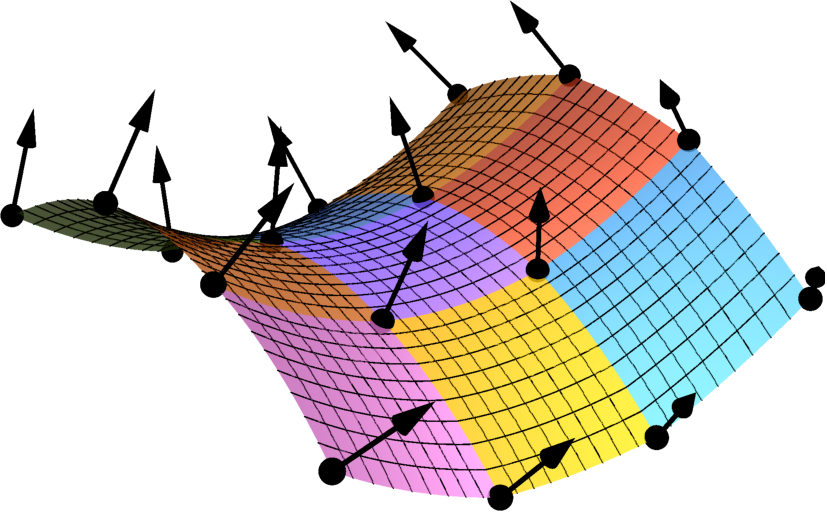
Example 4.3.
Consider 16 points , , and the associated unit normal vectors , see Fig. 5. The distribution of on shows again that also in this example it is possible to use the standard stereographic projection (50)
We project the unit vectors to plane, construct nine planar patches, see Fig. 4 (left), and lift them back to space, see Fig. 4 (right). Then, we construct nine polynomial patches of degree nine such that each patch corresponds to equations (45) and (46). Moreover we will consider equations:
| (62) |
Finally, by solving the whole system of linear equations we arrive at one-parametric solution. One particular solution is shown in Fig. 5.
Now we present how the designed approach can be easily adapted also for constructing smoothly joined triangular patches. The following example presents computing approximated polynomial PN parameterizations of patches on given surfaces, and thus also computing approximate (piecewise) polynomial PN parameterizations either of non-PN surfaces, or of PN surfaces with rational PN parameterizations only.
Example 4.4.
Consider the ellipsoid with the implicit equation
| (63) |
We approximate the ellipsoid with piecewise polynomial PN parametrization. In particular, we parameterize one octant corresponding to unit normal vectors:
| (64) |
and by symmetry, we find the remainder seven octants. Solving
| (65) |
yields two points for each normal vector. From each pair we choose one point such that all chosen points lie in the same octant, e.g.,
| (66) |
Next we interpolate vectors by a polynomial vector field fulfilling the Pythagorean property. In particular using stereographic projection (50) we project to the plane and in the plane we construct
| (67) |
as a rational triangular Bézier patch, see Fig. 6 (left).
Lifting via and omitting the denominator yields a Pythagorean normal vector field of bi-degree two. The vector field was constructed such that the symmetry yields a continuous normal vector field of the whole ellipsoid, see Fig. 6 (right).


Now we construct a PN surface (one triangular PN patch) of degree . Solving equations (45) and (46) together with equations
| (68) |
which guarantee a possibility to use the symmetry and thus to obtain all remaining seven patches, yields a -parametric solution. We choose the most suitable one by minimizing the following objective function
| (69) |
which is responsible for the deviation of the parametrization from the implicit surface . In this case we obtain the error smaller then . Finally using the symmetry we obtain the approximate piecewise polynomial PN parametric description of the whole ellipsoid (63), see Fig. 7.

Remark 4.5.
Let emphasize that when a higher continuity of the constructed interpolation piecewise polynomial surface is needed, then the presented method can be still applied. It is enough to increase the degree of the PN parameterizations (to have more free parameters) and add suitable extra continuity constrains (again linear equations) to the original linear system. Especially, when e.g. the continuity of the joint between two patches is required it is necessary to construct continuous normal vector fields (e.g. applying the bi-cubic Coons construction in the quadrilateral case, or cubic Clough-Tocher or quadratic Powell-Sabin elements in the triangular case).
4.2 Hermite interpolation by piecewise polynomial medial surface transforms yielding rational envelopes
The ideas formulated in the previous section for PN surfaces can be easily adapted also for Hermite interpolation with polynomial MOS surfaces. We present the approach at least for one quadrilateral and one triangular patch. We recall that interpolations by MOS surfaces can be used, for instance, when rational blending or skinning surfaces are constructed as the envelopes of two-parameter families of spheres.
Consider four points , , and four associated tangent planes determined by the vectors and . We find the ideal lines of , compute the conjugated lines with respect to (i.e., the ideal lines of the normal planes at ), and by intersecting them with the absolute quadric , cf. (33), we arrive at the isotropic vectors . Next, we interpolate the isotropic Gauss image (see Section 3.3), i.e., given data , by suitable rational patches and taking them as the input for (38) we arrive at an MOS patch interpolating given Hermite data .
Example 4.6.
Consider in the points
| (70) |
and the tangent vectors
| (71) |
determining the tangent planes at .
Then solving
| (72) |
yields the following isotropic normal vectors:
| (73) |
W.l.o.g, we choose for instance and compute the associated normals on the unit sphere , i.e.,
| (74) |
Next we interpolate data by a rational patch on the unit sphere , see Section 4.1, and finally we arrive at as the isotropic normal field interpolating data .
Then we prescribe a polynomial parameterization
| (75) |
of degree six and solve linear system of equations (34) together with the equations:
| (76) |
Let us emphasize that equations (76) must be added to ensure the prescribed interpolation conditions, i.e., that is tangent to at . Finally we obtain -parametric set of polynomial MOS surfaces of degree six interpolating given Hermite data , see Fig. 8 (left) for one particular example from the set of solutions.
The triangular patch would be treated analogously to the quadrilateral one, see the following example.
Example 4.7.
Consider in three points
| (77) |
and the three pairs of tangent vectors
| (78) |
determining the tangent planes at . By Solving (72) we arrive at the isotropic normal vectors:
| (79) |
Again, we choose e.g. , compute the associated normals on the unit sphere and construct the spherical triangular patch interpolating (see Section 4.1), i.e.,
| (80) |
Then we arrive at as the isotropic normal field interpolating data , where is given by (80).
Finally we prescribe a polynomial quartic parameterization (75) and solving linear system of equations (34) together with the equations (76) (now for ) yields -parametric set of quartic polynomial MOS surfaces interpolating given Hermite data , see Fig. 8 (right) for one chosen triangular patch from the set of all solutions.


5 Concluding remarks
In this paper the problem of Hermite interpolations by piecewise polynomial surfaces with polynomial area element was investigated. It was shown that the interpolation problem can be always transformed to solving a system of linear equations and the same approach is suitable not only for polynomial PN surfaces but also for polynomial MOS surfaces. Simplicity and functionality of the designed algorithm was presented on several examples. In our future work we would like to focus on better understanding of the quantity in (26) responsible for increasing free parameters in the construction, on the study of existence (or its eliminating) of the factor which causes vanishing of the normals along a curve on the surface, and finally on the construction of polynomial PN patches given by the boundary curves, which is a challenging open problem in geometric modelling.
Acknowledgments
The authors Michal Bizzarri, Miroslav Lávička and Jan Vršek were supported by the project LO1506 of the Czech Ministry of Education, Youth and Sports.
Appendix A Appendix
Let be the homogenization of the normal vector field , i.e., it is a triple of homogeneous polynomials of the same degree . As already mentioned earlier, the result depends on the occurrence of the base points of over . Denote the coordinate ring of . Analogously to we define which is a submodule of in this case.
Next, it is known that is a graded module over itself whose graded pieces are formed by the sets of homogeneous polynomials of degree . Obviously each is a finite–dimensional vector space over . For such a graded module , the Hilbert function is defined as
| (81) |
We introduce the standard notation for the shifted module, i.e., . Hence the Hilbert function of this module is
| (82) |
Let us emphasize that unlike the homogeneous syzygy module is not free anymore. The reason is that the basis of does not remain a basis of syzygy module after homogenization. To see this let be the homogenization of the vector field from Example 3.5. Then obviously but there is no way how to write it as -linear combination of
| (83) |
In fact is generated by , and . Nevertheless they do not form a basis because of the dependence relation .
Next let denote the ideal generated by the components of the normal field . Then there exists the so called Koszul complex
| (84) |
where the differentials are given by
| (85) |
This complex is known to be exact if and only if the sequence , , is regular. If admits the base points then the sequence cannot be regular. Nevertheless we have, cf. (Cox and Schenck, 2003)
Lemma A.1.
If has a codimension two in then complex (84) is exact except at .
Now we can formulate and prove the theorem that gives consequently a result presented in Section 3.2.
Theorem A.2.
Let be a homogeneous normal vector field of degree as above. Then
| (86) |
where the equality holds if and only if the normal field is basepoint-free.
Proof.
From (84) and (85) we immediately see that is the kernel of the map . Hence
| (87) |
where the term comes from the shift .
By Lemma A.1 complex (84) is exact except at , hence it is possible to express Hilbert function of the
| (88) |
Now is a submodule of and moreover if and only if has no base point. Thus we have where the equality occurs whenever the normal field is basepoint-free. Substituting (82) into (88) proves the theorem.
∎
References
- Alfeld et al. (1996) Alfeld, P., Neamtu, M., Schumaker, L. L., 1996. Fitting scattered data on sphere-like surfaces using spherical splines. Journal of Computational and Applied Mathematics 73 (1), 5–43.
- Bastl et al. (2008) Bastl, B., Jüttler, B., Kosinka, J., Lávička, M., 2008. Computing exact rational offsets of quadratic triangular Bézier surface patches. Computer-Aided Design 40, 197–209.
- Bastl et al. (2010) Bastl, B., Jüttler, B., Kosinka, J., Lávička, M., 2010. Volumes with piecewise quadratic medial surface transforms: Computation of boundaries and trimmed offsets. Computer-Aided Design 42 (6), 571–579.
- Bommes et al. (2013) Bommes, D., Lévy, B., Pietroni, N., Puppo, E., Silva, C., Tarini, M., Zorin, D., 2013. Quad-mesh generation and processing: A survey. Computer Graphics Forum 32 (6), 51–76.
- Chen et al. (2005) Chen, F., Cox, D., Liu, Y., 2005. The -basis and implicitization of a rational parametric surface. Journal of Symbolic Computation 39 (6), 689–706.
- Cox and Schenck (2003) Cox, D. A., Schenck, H., 2003. Local complete intersections in and Koszul syzygies. Proceedings of the American Mathematical Society 131 (7), 2007–2014.
- Dietz et al. (1993) Dietz, R., Hoschek, J., Jüttler, B., 1993. An algebraic approach to curves and surfaces on the sphere and on other quadrics. Computer Aided Geometric Design 10 (3-4), 211–229.
- Farin (1986) Farin, G., 1986. Triangular bernstein-bézier patches. Computer Aided Geometric Design 3 (2), 83–127.
- Farin (1988) Farin, G., 1988. Curves and Surfaces for Computer-Aided Geometric Design. Academic Press.
- Farouki (2008) Farouki, R., 2008. Pythagorean-Hodograph Curves: Algebra and Geometry Inseparable. Springer.
- Farouki and Sakkalis (1990) Farouki, R., Sakkalis, T., 1990. Pythagorean hodographs. IBM Journal of Research and Development 34 (5), 736–752.
- Farouki and Sakkalis (1994) Farouki, R., Sakkalis, T., 1994. Pythagorean-hodograph space curves. Advances in Computational Mathematics 2, 41–66.
- Farouki and Šír (2011) Farouki, R. T., Šír, Z., February 2011. Rational Pythagorean-hodograph space curves. Computer Aided Geometric Design 28, 75–88.
- Jüttler and Sampoli (2000) Jüttler, B., Sampoli, M., 2000. Hermite interpolation by piecewise polynomial surfaces with rational offsets. Computer Aided Geometric Design 17, 361–385.
- Kosinka and Jüttler (2007) Kosinka, J., Jüttler, B., 2007. MOS surfaces: Medial surface transforms with rational domain boundaries. In: The Mathematics of Surfaces XII. Vol. 4647 of Lecture Notes in Computer Science. Springer, pp. 245–262.
- Kosinka and Lávička (2010) Kosinka, J., Lávička, M., 2010. On rational Minkowski Pythagorean hodograph curves. Computer Aided Geometric Design 27 (7), 514–524.
- Kozak et al. (2016) Kozak, J., Krajnc, M., Vitrih, V., 2016. A quaternion approach to polynomial PN surfaces. Computer Aided Geometric Design(to appear).
- Kubota (1972) Kubota, K., 1972. Pythagorean triples in unique factorization domains. American Mathematical Monthly 79, 503–505.
- Lávička and Vršek (2012) Lávička, M., Vršek, J., 2012. On a special class of polynomial surfaces with Pythagorean normal vector fields. In: Boissonnat, J.-D., Chenin, P., Cohen, A., Gout, C., Lyche, T., Mazure, M.-L., Schumaker, L. (Eds.), Curves and Surfaces. Vol. 6920 of Lecture Notes in Computer Science. Springer Berlin Heidelberg, pp. 431–444.
- Lávička et al. (2016) Lávička, M., Šír, Z., Vršek, J., 2016. Smooth surface interpolation using patches with rational offsets. Computer Aided Geometric Design (submitted).
- Moon (1999) Moon, H., 1999. Minkowski Pythagorean hodographs. Computer Aided Geometric Design 16, 739–753.
- Peternell and Pottmann (1996) Peternell, M., Pottmann, H., 1996. Designing rational surfaces with rational offsets. In: Fontanella, F., Jetter, K., Laurent, P. (Eds.), Advanced Topics in Multivariate Approximation. World Scientific, pp. 275–286.
- Pottmann (1995) Pottmann, H., 1995. Rational curves and surfaces with rational offsets. Computer Aided Geometric Design 12 (2), 175–192.