Exact and Efficient Hamilton-Jacobi-based Guaranteed Safety Analysis via System Decomposition

For clarity, we assume that the state space $\mathcal{Z}$ is $\mathbb{R}^{n}$, but our theory also applies to systems with periodic state dimensions such as angles. The control is denoted by $u$, with the control function $u(\cdot)$ being drawn from the set of measurable functions¹¹ 1 A function $f:X\to Y$ between two measurable spaces $(X,\Sigma_{X})$ and $(Y,\Sigma_{Y})$ is said to be measurable if the preimage of a measurable set in $Y$ is a measurable set in $X$, that is: $\forall V\in\Sigma_{Y},f^{-1}(V)\in\Sigma_{X}$, with $\Sigma_{X},\Sigma_{Y}$ $\sigma$-algebras on $X$,$Y$.:

The system dynamics $f:\mathcal{Z}\times\mathcal{U}\rightarrow\mathcal{Z}$ is assumed to be uniformly continuous, bounded, and Lipschitz continuous in $z$ for fixed $u$. With this assumption, given $u(\cdot)\in\mathbb{U}$, there exists a unique trajectory solving (1) [20, 21].

We will denote solutions, or trajectories of (1) starting from some state $z$ at time $t$ under control $u(\cdot)$ as $\zeta(s;z,t,u(\cdot))$. The system trajectory satisfies an initial condition and the ODE (1) almost everywhere:

In this paper, we consider a common definition of the BRS relevant for guaranteeing safety. Intuitively, the BRS represents the set of states $z$ from which the system can be driven into an unsafe set $\mathcal{L}$ at a particular time. For our definition of BRS, we stipulate that the system be driven to $\mathcal{L}$ for all control functions $u(\cdot)$. In this case, the unsafe set can often be interpreted as a set of states to be avoided (such as an obstacle), and the BRS represents the set of states that leads to the system entering the unsafe set despite all possible control functions. We now formally define the BRS.

There are various similar HJ formulations such as [1, 2, 4], and [22] that cast the reachability problem as an optimal control problem and directly compute the BRS in the full state space of the system. These numerical solutions to the optimal control problem involve solving an HJ PDE on a grid that represents a discretization of the state space. Although these methods are not scalable beyond relatively low-dimensional systems, they form the foundation on which we will build our theory. We now briefly summarize the necessary details related to the HJ PDEs, and what their solutions represent in terms of the cost function and value function of the corresponding optimal control problem.

Let the unsafe set $\mathcal{L}\subseteq\mathcal{Z}$ be represented by the implicit surface function $l(z)$ such that the unsafe set is the zero sub-level set of the implicit surface function: $\mathcal{L}=\{z\in\mathcal{Z}:l(z)\leq 0\}$. Such a function always exists since we can choose $l(\cdot)$ to be the signed distance function from $\mathcal{L}$. Examples of implicit surface functions are shown as colored surfaces in Fig. 1, with the boundary of the corresponding sets they represent shown in black.

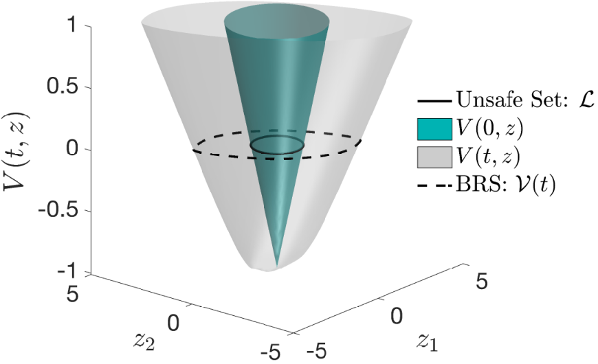
Consider the optimal control problem given by

It is well-known that the value function $V(t,z)$ is the implicit surface function representing $\mathcal{V}(t)$: $\mathcal{V}(t)=\{z\in\mathcal{Z}:V(t,z)\leq 0\}$.

The value function $V(t,z)$ is the viscosity solution [23, 24] of the HJ PDE

The Hamiltonian in (7) is given by

Fig. 1 shows an illustration of HJ reachability. $l(z)$, the implicit surface function representing $\mathcal{L}$, and the value function $V(t,z)$, the implicit surface function representing the BRS $\mathcal{V}(t)$, are shown as the blue and light gray surfaces respectively. The unsafe set $\mathcal{L}$ and the BRS $\mathcal{V}(t)$ are the zero sub-level sets of these two surface functions; the boundaries of $\mathcal{L}$ and $\mathcal{V}(t)$ are shown in black. Once the value function $V$ is computed, the optimal control (6) can be obtained by the expression

We state the following algorithm for clarity and convenience:

We assume that the full system unsafe set $\mathcal{L}$ can be written in terms of the subsystem unsafe sets $\mathcal{L}_{x_{1}}\in\mathcal{X}_{1},\mathcal{L}_{x_{2}}\in\mathcal{X}_{2}$ in the way depicted in Fig. 3:

Next, we define the subsystem BRSs $\mathcal{V}_{x_{1}},\mathcal{V}_{x_{2}}$ the same way as in (4), but with the subsystems in (12) and subsystem unsafe sets $\mathcal{L}_{x_{1}},\mathcal{L}_{x_{2}}$, respectively:

Given a system in the form of (12) with unsafe set that can be represented by (21), our goal is to compute the full-dimensional BRS by performing computations in the lower-dimensional subspaces. Specifically, we would like to first compute the subsystem BRSs $\mathcal{V}_{x_{1}}(t),\mathcal{V}_{x_{2}}(t)$, and then construct the full system BRS $\mathcal{V}(t)$ exactly. This process dramatically reduces computation complexity by decomposing the higher-dimensional system into two lower-dimensional subsystems. Specifically, we will show that if the unsafe set can be decomposed in the way described by (21), then the full-dimensional BRS is decomposable in the same way:

It is important to note that if the subsystem states $x_{1},x_{2}$ have no overlapping states (and are therefore decoupled), the above statement is relatively intuitive and easy to show; however, when the subsystems have the overlapping states in the partition $y_{3}$, they are coupled to each other through these overlapping states. Our main result in this paper proves that despite this coupling, (23) still holds.

The Dubins Car is a well-known system whose dynamics are given by (13). This system is only 3D, and its BRS can be tractably computed in the full-dimensional space, so we use it to compare the full formulation with the SCS formulation.

As previously mentioned, the Dubins Car dynamics can be decomposed according to (14).

For this example, we computed the BRS from the unsafe set representing the set of positions near the origin in both the $p_{x}$ and $p_{y}$ dimensions. More concretely, our unsafe set was defined to be $\mathcal{L}=\{(p_{x},p_{y},\theta):|p_{x}|,|p_{y}|\leq 0.5\}$. Such an unsafe set can be used to model an obstacle that the vehicle must avoid. Given the unsafe set, the interpretation of the BRS $\mathcal{V}(t)$ is the set of states from which a collision with the obstacle may occur after a duration of $t$.

From $\mathcal{L}$, we computed the BRS $\mathcal{V}(t)$ of time horizon $t=0.5$. The resulting full formulation BRS is shown in Fig. 4 as the red surface which appears in the two subplots on the right.

To compute the BRS using the SCS formulation, note that the unsafe set $\mathcal{L}$ can be written as $\mathcal{L}=\text{proj}^{-1}(\mathcal{L}_{x_{1}})\cap\text{proj}^{-1}(\mathcal{L}_{x_{2}})$, with

From these lower-dimensional unsafe sets, we computed the lower-dimensional BRSs $\mathcal{V}_{\mathcal{X}_{1}}(t)$ and $\mathcal{V}_{\mathcal{X}_{2}}(t)$, and then constructed the full-dimensional BRS $\mathcal{V}(t)$ using Theorem 1: $\mathcal{V}(t)=\text{proj}^{-1}(\mathcal{V}_{x_{1}}(t))\cap\text{proj}^{-1}(\mathcal{V}_{x_{2}}(t))$. The subsystem BRSs and their back projections are shown in magenta and green in the left subplot of Fig. 4. The constructed BRS is shown in the three left subplots of Fig. 4 as the black mesh.

In the middle-right plot of Fig. 4, we superimpose the full-dimensional BRS computed using the two methods. We show the comparison of the computation results viewed from several different angles in Fig. 5. The results are indistinguishable. However, when using the SCS formulation, Theorem 1 allows the computation to be done significantly faster in lower-dimensional subspaces. An additional benefit of the SCS formulation is that in the numerical methods for solving the HJ PDE, the amount of numerical dissipation increases with the number of state dimensions. Thus, computations in lower-dimensional subspaces lead to a slightly more accurate numerical solution.

The computation benefits of using the SCS formulation can be seen from Fig. 6. Both subplots show the computation time in seconds versus the number of grid points per dimension in the numerical computation. From the top subplot, one can easily see that the direct computation of the full formulation BRS in 3D becomes very time-consuming as the number of grid points per dimension is increased, while the computation using the SCS formulation hardly takes any time in comparison. The bottom subplot shows the same data, but on a log-log scale for more detail. Directly computing the BRS with 251 grid points per dimension using the full formulation took approximately 80 minutes, while computing the BRS using the SCS formulation is faster by several orders of magnitude: the computation only took approximately 30 seconds! The computations were timed on a desktop computer with an Intel Core i7-2600K processor and 16GB of random-access memory.

This example illustrates the ability of the SCS formulation to produce BRSs for high-dimensional systems that would be otherwise intractable to analyze by current HJ-based methods. In [25], a 6D Acrobatic Quadrotor model used to perform backflips was simplified into a series of smaller hybrid models due to the intractability of computing a BRS over a 6D state space. Using the new SCS formulation we can accurately compute a BRS for the full 6D system.

The 6D Acrobatic Quadrotor’s state is $z=(p_{x},v_{x},p_{y},v_{y},\phi,\omega)$; the dynamics are given by [25]:

The state partitions of this system are $y_{1}=(p_{x},v_{x}),y_{2}=(p_{y},v_{y}),y_{3}=(\phi,\omega)$. Using the SCS formulation, we decompose the full system into the following set of subsystems:

For this example we will compute the BRS that describes the set of initial conditions from which the system may enter the unsafe set after a given time period $t$ despite best possible control. We define the unsafe set as a square of length 1m centered at $(p_{x},p_{y})=(0,0)$ described by $\mathcal{L}=\{(p_{x},v_{x},p_{y},v_{y},\phi,\omega):|p_{x}|,|p_{y}|\leq 1\}$. This can be interpreted as a positional box centered at the origin that must be avoided for all angles and velocities. From the unsafe set, we define $l(z)$ such that $l(z)\leq 0\Leftrightarrow x\in\mathcal{L}$. This unsafe set must be decomposed to provide a suitable unsafe set for each subsystem. This is done by letting $\mathcal{L}_{x_{i}},$ $i=1,2$ be

The BRS of each 4D subsystem is computed and then combined into the 6D BRS using the SCS formulation. To visually depict the 6D BRS, 3D slices of the BRS along the positional and velocity axes were computed. Fig. 7 shows a 3D slice in $(p_{x},p_{y},\phi)$ space at $v_{x}=v_{y}=1$ m/s, $\omega=0$ rad/s. The dark blue set represents the unsafe set $\mathcal{L}$, with the BRS in light blue.

In Fig. 8, 3D slices in $(v_{x},v_{y},\omega)$ space are visualized at $p_{x},p_{y}=1.5$ m, $\phi=1.5$ rad. These colored sets represent the BRS at different points in time.

References

- [1] E. N. Barron, “Differential Games with Maximum Cost,” Nonlinear analysis: Theory, methods & applications, pp. 971–989, 1990.
- [2] I. M. Mitchell, A. M. Bayen, and C. J. Tomlin, “A time-dependent Hamilton-Jacobi formulation of reachable sets for continuous dynamic games,” IEEE Transactions on Automatic Control, vol. 50, no. 7, pp. 947–957, July 2005.
- [3] K. Margellos and J. Lygeros, “Hamilton-Jacobi Formulation for Reach-Avoid Differential Games,” IEEE Transactions on Automatic Control, vol. 56, no. 8, Aug 2011.
- [4] O. Bokanowski and H. Zidani, “Minimal time problems with moving targets and obstacles,” {IFAC} Proceedings Volumes, vol. 44, no. 1, pp. 2589 – 2593, 2011.
- [5] J. Ding, J. Sprinkle, S. S. Sastry, and C. J. Tomlin, “Reachability calculations for automated aerial refueling,” in IEEE Conference on Decision and Control, Cancun, Mexico, 2008.
- [6] E. M. Vaisbord and V. I. Zhukovskii, Introduction to Multi-player Differential Games and Their Applications. Routledge, 1988.
- [7] I. Mitchell, “Application of level set methods to control and reachability problems in continuous and hybrid systems,” Ph.D. dissertation, Stanford University, 2002.
- [8] J. A. Sethian, “A fast marching level set method for monotonically advancing fronts,” Proceedings of the National Academy of Sciences, vol. 93, no. 4, pp. 1591–1595, 1996.
- [9] S. Osher and R. Fedkiw, Level Set Methods and Dynamic Implicit Surfaces. Springer-Verlag, 2002.
- [10] I. Mitchell, A Toolbox of Level Set Methods, 2009. [Online]. Available: http://people.cs.ubc.ca/ mitchell/ToolboxLS/index.html
- [11] A. Majumdar and R. Tedrake, Algorithmic Foundations of Robotics X: Proceedings of the Tenth Workshop on the Algorithmic Foundations of Robotics. Springer Berlin Heidelberg, 2013, ch. Robust Online Motion Planning with Regions of Finite Time Invariance, pp. 543–558.
- [12] T. Dreossi, T. Dang, and C. Piazza, “Parallelotope bundles for polynomial reachability,” in 19th International Conference on Hybrid Systems: Computation and Controls, 2016.
- [13] A. B. Kurzhanski and P. Varaiya, “Ellipsoidal techniques for reachability analysis: internal approximation,” Systems & control letters, vol. 41, no. 3, pp. 201–211, 2000.
- [14] J. N. Maidens, S. Kaynama, I. M. Mitchell, M. M. Oishi, and G. A. Dumont, “Lagrangian methods for approximating the viability kernel in high-dimensional systems,” Automatica, July 2013.
- [15] J. Darbon and S. Osher, “Algorithms for overcoming the curse of dimensionality for certain hamilton-jacobi equations arising in control theory and elsewhere,” arXiv preprint arXiv:1605.01799, 2016.
- [16] I. M. Mitchell and C. J. Tomlin, “Overapproximating reachable sets by hamilton-jacobi projections,” Journal of Scientific Computing, vol. 19, no. 1-3, pp. 323–346, 2003.
- [17] M. Chen*, S. Herbert*, and C. J. Tomlin, “Fast reachable set approximations via state decoupling disturbances,” in 55th IEEE Conference on Decision and Control, 2016.
- [18] I. M. Mitchell, “Scalable calculation of reach sets and tubes for nonlinear systems with terminal integrators: A mixed implicit explicit formulation,” in Proceedings of the 14th International Conference on Hybrid Systems: Computation and Control, 2011, pp. 103–112.
- [19] J. F. Fisac, M. Chen, C. J. Tomlin, and S. S. Shankar, “Reach-avoid problems with time-varying dynamics, targets and constraints,” in 18th International Conference on Hybrid Systems: Computation and Controls, 2015.
- [20] L. C. Evans and P. E. Souganidis, “Differential games and representation formulas for solutions of Hamilton-Jacobi-Isaacs equations,” Indiana Univ. Math. J., vol. 33, no. 5, pp. 773–797, 1984.
- [21] E. A. Coddington and N. Levinson, Theory of ordinary differential equations. Tata McGraw-Hill Education, 1955.
- [22] P. Varaiya, “On the existence of solutions to a differential game,” SIAM Journal on Control, vol. 5, no. 1, pp. 153–162, 1967.
- [23] M. G. Crandall and P.-L. Lions, “Viscosity solutions of Hamilton-Jacobi equations,” Transactions of the American Mathematical Society, vol. 277, no. 1, pp. 1–42, 1983.
- [24] M. G. Crandall, L. C. Evans, and P. L. Lions, “Some properties of viscosity solutions of hamilton-jacobi equations,” Transactions of the American Mathematical Society, vol. 282, no. 2, p. 487, April 1984.
- [25] J. H. Gillula, G. M. Hoffmann, H. Huang, M. P. Vitus, and C. J. Tomlin, “Applications of hybrid reachability analysis to robotic aerial vehicles,” International Journal of Robotics Research, vol. 30, no. 3, pp. 335–354, March 2011.