A Computation in a Cellular Automaton Collider Rule 110
Abstract
A cellular automaton collider is a finite state machine build of rings of one-dimensional cellular automata. We show how a computation can be performed on the collider by exploiting interactions between gliders (particles, localisations). The constructions proposed are based on universality of elementary cellular automaton rule 110, cyclic tag systems, supercolliders, and computing on rings.
0.1 Introduction: Rule 110
Elementary cellular automaton (CA) rule 110 is the binary cell state automaton with a local transition function of a one-dimensional (1D) CA order in Wolfram’s nomenclature [57], where is the number of cell states and the number of neighbours of a cell. We consider periodic boundaries, i.e. first and last cells of a 1D array are neighbours. The local transition function for rule 110 is defined in Tab. 0.1, the string 01101110 is the number 110 in decimal notation:
| (1) | ||||

A cell in state ‘0’ takes state ‘1’ if both its neighbours are in state ‘1’ or left neighbour is ‘0’ and right neighbour is ‘1’; otherwise, the call remains in the state ‘0’. A cell in state ‘1’ takes state ‘0’ if both its neighbours are in state ‘1’, or both its neighbours are in state ‘0’ or it left neighbour is ‘1’ and its right neighbour is ‘0’. Fig. 1 shows an evolution of rule 110 from a random initial condition. We can see there travelling localisation: particles or gliders, and some stationary localisations: breathers, oscillators or stationary structures.
0.1.1 System of particles
A detailed description of particles/gliders discovered in evolutions of CA rule 110 is provided in [32, 36].11 1 See also, http://uncomp.uwe.ac.uk/genaro/rule110/glidersRule110.html Further, we refers to a train of copies of particle as .

| Margins | ||||||
| Structure | Left – Right | Velocity | Lineal | |||
| Volume | ||||||
| \svhline | . | 1 | . | 1 | 2/3 0.666666 | 14 |
| 1 | . | 1 | . | -1/2 = -0.5 | 14 | |
| . | 1 | . | 1 | 2/3 0.666666 | 6 | |
| 1 | . | 1 | . | -2/4 = -0.5 | 8 | |
| 3 | . | 3 | . | -6/12 = -0.5 | 22 | |
| 3 | . | 3 | . | -6/12 = -0.5 | 39 | |
| 1 | 1 | 1 | 1 | 0/7 = 0 | 9-23 | |
| 1 | 1 | 1 | 1 | 0/7 = 0 | 17 | |
| 1 | 1 | 1 | 1 | 0/7 = 0 | 11 | |
| 1 | 2 | 1 | 2 | 2/10 = 0.2 | 11-25 | |
| 1 | 2 | 1 | 2 | 2/10 = 0.2 | 19 | |
| 3 | 1 | 3 | 1 | -4/15 -0.266666 | 19 | |
| 6 | 2 | 6 | 2 | -8/30 -0.266666 | 21 | |
| 6 | 4 | 6 | 4 | -4/36 -0.111111 | 15-29 | |
| 9 | 2 | 9 | 2 | -14/42 -0.333333 | 24-38 | |
| 17 | 8 | 17 | 8 | -18/92 -0.195652 | 39-53 | |
| glider gun | 15 | 5 | 15 | 5 | -20/77 -0.259740 | 27-55 |
Figure 2 shows all known particles, and generators of particles, or glider guns. Each particle has its unique features, e.g. slopes, velocities, periods, contact points, collisions, and phases [37, 35, 33]. A set of particles in rule 110 is defined as:
where means that a structure of the particle can be extendible infinitely, the rest of symbols denote types of particles as shown in Fig. 2. Table 1 summarizes key features of the particles: column structure gives the name of each particle including two more structures: and which represent the slopes of ether pattern (periodic background). The next four columns labeled margins indicate the number of periodic margins in each particle: they are useful to recognize contact points for collisions. The margins are partitioned in two types with even values ems and odd values oms which are distributed also in two groups: left and right margins. Column indicates a velocity of a particle , where belongs to a particle of the set of particles G. A relative velocity is calculated during the particle’s displacement on cells during period . We indicate three types of a particle propagation via sign of its velocity. A particle travelling to the right has positive velocity, a particle travelling to the left has negative velocity. Stationary particle has zero velocity. Different velocities of particles allow us to control distances between the particle to obtained programmable reactions between the particles. Typically, larger particles has lower velocity values. No particle can move faster than or . Column lineal volume shows the minimum and maximum number of necessary cells occupied by the particle.
0.1.2 Particles as regular expressions
We represent CA particles as strings. These strings can be calculated using de Bruin diagrams [31, 34, 55, 32, 37] or with the tiles theory [16, 33, 35, 37]. 22 2 See a complete set of regular expressions for every particle in rule 110 in http://uncomp.uwe.ac.uk/genaro/rule110/listPhasesR110.txt
A regular language is based on a set of regular expressions uniquely describing every particle of G. A subset of the set of regular expressions
| (2) |
where is a period, determines the language
| (3) |
From these set of strings we can code initial configurations to program collisions between particles [39, 27, 36].

To deriver the regular expressions we use the de Bruijn diagrams [31, 55, 34] as follows. Assume the particle moves two cells to the right in three time steps (see Tab. 1). The corresponding extended de Bruijn diagram (2-shift, 3-gen) is shown in Fig. 3. Cycles in the diagram are periodic sequences uniquely representing each phase of the particle. Diagram in Fig. 3 has two cycles: a cycle formed by just a vertex 0 and another large cycle of 26 vertices composed by other nine internal cycles. The sequences or regular expressions determining the phases of the particle are obtained by following paths through the edges of the diagram. There regular expressions and corresponding paths in Bruijn diagram are shown below.
- I.
The expression (1110)*: vertices 29, 59, 55, 46 determining particles.
- II.
The expression (111110)*: vertices 61, 59, 55, 47, 31, 62 defining particles with a tile among each particle.
- III.
The expression (11111000100110)*: vertices 13, 27, 55, 47, 31, 62, 60, 56, 49, 34, 4, 9, 19, 38 describing the periodic background configurations in a specific phase.
Cycle with period 1 (vertex 0) yields a homogeneous evolution in state 0. The evolution space in Fig. 3 shows different trains of particles. The initial condition is constructed following some of the seven possible cycles of the de Bruijn diagram or a combination of them. In this way, the number of particles or the number of intermediate tiles can be selected by moving from one cycle to another.
The alignment of the fi_1 phases is analysed to determine the whole set of strings for every particle. We describe the form and limits of each particle by tiles. Then a phase is fixed (in our case the phase fi_1) and a horizontal line is placed in the evolution space bounded by two aligned tiles. The sequence between both tiles aligned in each of the four levels determines a periodic sequence representing a particular structure in the evolution space of rule 110. All periodic sequences in a specific phase are calculated, enumerating the phases for each particle or non-periodic structure.
| phases level one () | f1_1, f2_1, f3_1, f4_1 | |
| phases level two () | f1_2, f2_2, f3_2, f4_2 | |
| phases level three () | f1_3, f2_3, f3_3, f4_3 | |
| phases level four () | f1_4, f2_4, f3_4, f4_4 |
Table 2 represents disjoint subset of phases, each level contains four phases. Variable fi indicates the phase of a particle, and the subscript (in the notation fi_) indicates the selected set of regular expressions. Finally, we use the next notation to codify initial conditions by phases as follows:
| (4) |
where #1 represents a particle according to Cook’s classification (Table 1) and #2 is a phase of the particle with period greater than four.
0.2 Universal elementary CA
A concept of universality and self-reproduction in CA was proposed by von Neumann in [54] in his design of a universal constructor in a 2D CA with 29 cell-states. Architectures of universal CA have been simplified by Codd in 1968 [10], Banks in 1971 [7], Smith in 1971 [51], Conway in 1982 [8], Lindgren and Nordahl in 1990 [22], and Cook in 1998 [11].33 3 A range of universal CA is listed here http://uncomp.uwe.ac.uk/genaro/Complex_CA_repository.html Cook simulated a cyclic tag system, equivalent to a minimal Turing machine, in CA rule 110. In general, computation capacities are explores in complex CA and chaotic CA [40].
0.3 Cyclic tag systems
Cyclic tag systems are used by Cook in [11] as a tool to implement computations in rule 110. Cyclic tag systems are modified from tag systems by allowing the system to have the same action of reading a tape in the front and adding characters at its end:
- 1.
Cyclic tag systems have at least two letters in their alphabet ().
- 2.
Only the first character is deleted () and its respective sequence is added.
- 3.
In all cases if the machine reads a character zero then the production rule is always null (, where represents the empty word).
- 4.
There are sequences from which are periodically accessed to specify the current production rule when a nonzero character is taken by the system. Therefore the period of each cycle is determinate by .
Such cycle determines a partial computation over the tape, although a halt condition is not specified. Let us see some samples of a cyclic tag system working with , and the following production rules: , and . To avoid writing a chain when there is no need to add characters, the relation is just indicated. For example, the 00001 represents the relations 00001 0001 001 01 1 10. Each relation indicates which exactly sequence is selected.
Cyclic tag systems tend to growth quickly which makes it difficult to analyse their behaviour. Morita in [43, 44] demonstrated how to implement a particular halt condition in cyclic tag systems given an output string when the system is halting, and how a partitioned CA can simulate any cyclic tag system, consequently computing all the recursive functions.
Similar to Post’s developments with tag systems, Cook determined that for a cyclic tag system with , , the productions and , and starting evolution with the state 1 on the tape, it is impossible to decide if the process is terminal.
0.4 Cyclic tag system working in rule 110
Let us see how a cyclic tag system operates in rule 110 [58]. We use a cyclic tag system with , and the productions and , starting its evolution in state 1 on the tape. A fragments of the systems’ behaviour is shown below:
1 11 110 1011 01110 11010 101011 0101110 0111010 1101010 10101011 010101110 010111010 011101010 110101010 1010101011 01010101110 01010111010 01011101010 01110101010 11010101010 101010101011 0101010101110 0101010111010 01010111010 10 0101110101010 0111010101010 1101010101010 10101010101011 010101010101110 010101010111010 01010 1011101010 010101110101010 010111010101010
We start with the expression 1(10)*. The cyclic tag systems moves (from the right to the left) and adds a pair of bits. As soon as the expression 1(10)* appears again, a number of relations selected in each interval in such a manner that the expressions grow lineally in order of .

If we take consecutive copies of 1(10)* with their respective intervals determined by the number of productions (represented as ), we obtain the following sequence: 1 110 11010 1101010 1101010 110101010 11010101010 1101010101010 . There are no states where to ‘0’ appear together.
Further, we show how to interpret particles and their collisions to emulate a cyclic tag system in rule 110. We must use trains of particles to represent data and operators, their reactions, transform and deletion of data on the tape. A schematic diagram, where trains of particles are represented by lines, is shown in Fig. 4. The diagram is explained with details in the next sections.
0.4.1 Components based on sets of particles
A construction of the cyclic tag system in rule 110 can be subdivided into three parts (Fig. 4). First part is the left periodic part controlled by trains of 4_ particles. This part is static. It controls the production of ’s and ’s. The second part is the center determining the initial value on the tape. The third part is the right, cyclic, part which contains the data to process. It adds or removes data on the tape.
Set of particles 4_
The four trains of particles are static but their phases change periodically. A key point is to implement these components by defining both distances and phases, because some choices of phases or distances might induce an undesirable reactions between the trains of particles.

Packages defined by particles have three different phases: f1_1, f2_1 and f3_1. To construct the first train 4_ we must establish the phase of each . Let us assign phases as follows:
(f3_1)--(f2_1)--(f1_1)--(f3_1),
see Fig. 5. Spaces between each train 4_ are fixed but the phases change. The soliton-like collisions between the particles occur:
{-(f2_1)--(f1_1)--(f3_1)--(f2_1)--(f1_1)-
-(f3_1)--(f2_1)--(f1_1)]--(f3_1)--(f2_1)--
(f1_1)--(f3_1)}*
If for every 4_ we take a phase representing the complete train, we can rename it as:
{-4_(F2)--4_(F1)--4_(F3)}*
this phase change is important to preserve good reactions coming to the left side of the system.
Set of particles 1Ele and 0Ele
The central part is made of the state ‘1’ written on the tape represented by a train of four particles. A set of particles 1Ele represents ‘1’ and a set of particles 0Ele represents ‘0’ on the tape.

The left configurations in Fig. 6 shows the set of particles 1Ele. We should reproduce each set of particles by the phases fi_1. The phases are coded as follows: (A,f1_1)--(A,f1_1)--(A,f1_1)--(B,f2_1). The first three particles are in phase (A,f1_1) and the fourth particle is in phase (B,f2_1). The distances between the particles are --. To determine the distances, we count the number of tiles between particles. Similarly, we obtain the distances -- for the particles 0Ele.
Set of particles 0Blo
The left part stores blocks of data without transformations in trains of and the particles .

The set of particles 0Blo is formed by 12 particles as we can see in Fig. 7. There must be an exact phase and distance between each one of the particles, otherwise the whole system will be disturbed.
Set of particles 1BloP and 1BloS
To write ‘1’s we must use two set of particles — primary and standard.

They are differences in distance between first two particles , as shown in Fig. 8. Both blocks produce the same set of particles 1Add. The main reason to use both set of particles is because the CA rule 110 evolves asymmetrically and therefore we need a double set of particles to produce values 1 correctly.
Set of particles SepInit

A leader component renamed as the set of particles SepInit (see Fig. 9) is essential to separate trains of data and to determine the incorporation of the data on the tape. Its has a small but detailed code determining which data without transformation would be added or erased from the tape, depending on the value that is coming.
Set of particles 1Add and 0Add
Figure 10 illustrates the set of particles 1Add and 0Add produced by two previous different trains of data. A set of particles 1Add must be generated by the set of particles 1BloP or 1BloS. This way, both set of particles can produce the same element.

On the other hand, a set of particles 0Add is generated by a set of particles 0Blo. Nevertheless, we could produce particles modifying their first two distances and preserving them without changing others particles to get a reliable reaction. This is possible if we want to experiment with other combinations of blocks of data.
If a leader set of particles SepInit reaches a set of particles 1Ele, it erases this value from the tape and adds a new data that shall be transformed. In other case, if it finds a set of particles 0Ele, then it erases this set of particles from the tape and also erases a set of unchanged data which comes from the right until finding a new leader set of particles. This operation represents the addition of new values from periodic trains of particles coming from the right. Thus a set of particles 1Add is transformed into 1Ele colliding against a train of 4 particles representing a value 1 in the tape, and the set of particles 0Add is transformed into 0Ele colliding against a train of 4 particles representing a value 0 in the tape.
| set of particles | distance |
|---|---|
| 1Ele | 9-9-7 |
| 0Ele | 9-5-7 |
| 1BloP | 4-6-2-8-8-2-10-1-2-8-8 |
| 1BloS | 10-1-2-8-8-2-10-1-2-8-8 |
| 0Blo | 10-1-2-8-8-8-10-1-2-8-8 |
| SepInit | 4-14--6-9-2-8 |
| 1Add | 27-21-27 |
| 0Add | 27-27-27 |
Table 3 shows all distances (in numbers of tiles) for every. We can code the construction of this cyclic tag system across phase representations in three main big sub systems:
left: … --4(F2)--4(F1)--4(F3)--4(F2)- -4(F1)--4(F3)-- center: 1Ele(A,f1_1)--(f1_1)- right: SepInit(C,f3_1)-1BloP(C,f4_1)-SepInit(C,f3_1)- 1BloP(C,f4_1)-0Blo(C,f4_1)-1BloS(A,f4_1)- SepInit(A,f2_1)(2)-1BloP(F,f1_1)-SepInit(A,f3_1)(2)- 1BloP(F,f1_1)-0Blo(E,f4_1)-1BloS(C,f4_1)-- SepInit(B,f1_1)(2)-1BloP(F,f3_1)-- SepInit(B,f1_1)(2)--….
The initial conditions in rule 110 are able to generate the serial sequence of bits 1110111 and a separator at the end with two particles. A desired construction is achieved in 57,400 generations and an initial configuration of 56,240 cells. The whole evolution space is 3,228,176,000 cells. See details [38].
0.4.2 Simulating a cyclic tag system in rule 110
The cyclic tag system starts with the value ‘1’ on the tape, see Fig. 4. We show a selection of snapshots of the machine working in rule 110 (see details in [38, 47]). We show different sets of particles with coloured labels on the snapshot below.

Figure 11 shows the initial stage of the cyclic tag system with the state ‘1’ in the tape. This data is represented by the set of particles 1Ele. The snaphshot shows a central part of the machine and a train of particles. We can see the first leader in the set of particles SepInit coming from the right periodic side.

The first reaction in Fig. 11 deletes the state ‘1’ on the tape. The set of particles 1Ele) and the particles’ separator are prepared for next data to be aggregated. If a set of particles 0Ele is encountered on the tape then data is not added to the tape until another separator appears. The particles left after the first production are invisible to the system, they do not affect any operations because they cross as solitons, without state modifications, the subsequent set of particles 4.

In Fig. 12 we see a set of particles 1Ele constructed from a train of particles 4. These particles have a very short life because quickly a separator set of particles arrives. This separator erases the particles and prepares new data that would be aggregated to the tape.

Figure 13 presents the construction of a set of particles 1Ele. In this stage of the evolution, we can see how data is aggregated, based on their values, before they cross the tape. Similar reactions can be observed with the set of particles 0Ele.
Figure 14 shows a constructed a set of particles 0Ele and its roles in the system. At the top, a set of particles 1Add, previously produced by a standard component 1BloS, crosses a set of particles 0Ele. A leader set of the particles deletes ‘0’ from the tape and all the subsequent incoming data. There are 1BloP, 0Blo and 1BloS set of particles in the illustrated sequence. The tile is generated in the process. This differences in distances between the particles determine a change of phases which will lead to erasure of particles , instead of production of particles . The reaction is used to delete the particles.
Production rules in cyclic tag system specify that for the state ‘0’ the first element of the chain must be erased and the other elements are conserved and no data are written on the tape. If the state is ‘1’ the first element of the chain is deleted and 10 or 11 are aggregated depending of the value. This behaviour is particularly visible when a separator finds 0 or 1 and deletes it from the tape. If the deleted data is ‘0’, a separator does not allow the production of new data. If the deleted data is ‘1’ the separator aggregates new elements 11 or 10, which are modified at later stages of the system’s development. Using this procedure, we can calculate up to the sixth ‘1’ of the sequence 01110 produced by the cyclic tag system.
In terms of periodic phases, this cyclic tag system working in rule 110 can be simplified as follows:
left: {-4(F)}*, for in sequential order center: -1EleC2(A,f1_1)--(f1_1) right: {SepInit(#,fi_1)-1BloP(#,fi_1)-SepInit(#,fi_1)- 1BloP(#,fi_1)-0Blo(#,fi_1)-1BloS(#,fi_1)}* (where and # represents a particular phase).
These periodic coding will be very useful to design and synchronise three interlinked rings of 1D CA (cyclotrons) to make a ‘supercollider’.
0.5 Cellular automata supercollider
In the late 1970s Fredkin and Toffoli proposed a concept of computation based on ballistic interactions between quanta of information that are represented by abstract particles [53]. The Boolean states of logical variables are represented by balls or atoms, which preserve their identity when they collide with each other. Fredkin, Toffoli and Margolus developed a billiard-ball model of computation, with underpinning mechanics of elastically colliding balls and mirrors reflecting the balls’ trajectories. Margolus proposed a special class of CA which implements the billiard-ball model [24]. Margolus’ partitioned CA exhibited computational universality because they simulated Fredkin gates via collision of soft spheres [26, 25]. Also, we consider previous results about circular machines designed by Arbib, Kudlek, and Rogozhin in [5, 20, 21]. Initial reports about CA collider were published in [30, 28, 29].
The following functions with two input arguments and can be realised in collisions between two localizations:
[]
To represent Toffoli’s supercollider [53] in 1D CA we use the notion of an idealised particle (without energy and potential). The particle is represented by a binary string of cell states.
[]


Figure 16 shows two typical scenarios where particles and travel in a CA cyclotron. The first scenario (Fig. 16a) shows two particles travelling in opposite directions; these particles collide one with another. Their collision site (contact point) is shown by a dark circle in Fig. 16a. The second scenario demonstrates a beam routing where a fast particle eventually catches up with a slow particle at a collision site (Fig. 16b). If the particles collide like solitons, then the faster particle simply overtakes the slower particle and continues its motion (Fig. 16c).
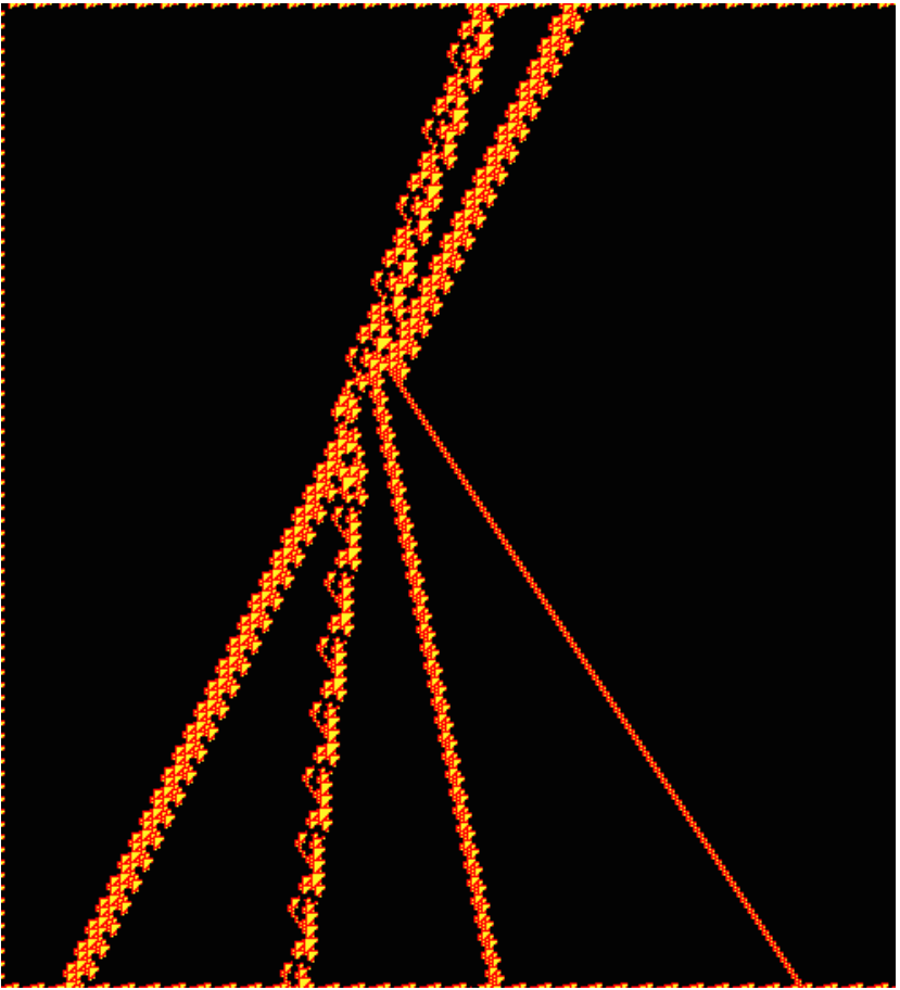
Typically, we can find all types of particles in complex CA, including particles with positive , negative , and neutral displacements, and composite particles assembled from elementary localizations. A sample coding and colliding particles is shown in Fig. 17, which displays a typical collision between two particles in rule 110. As a result of the collision one particle is split into three different particles (for full details please see [35]). The previous collision positions of particles determines the outcomes of the collision. Particles are represented now with orientation and name of the particle in rule 110 as follows: .
[]


To represent particles on a given beam routing scheme (see Fig. 16), we do not consider the periodic background configuration in rule 110 because essentially this does not affect on collisions. Fig. 18 displays a 1D configuration where two particles collide repeatedly and interact as solitons so that the identities of the particles are preserved in the collisions. A negative particle collides with and overtakes a neutral particle . First cyclotron (Fig. 18a) presents a whole set of cells in state 1 (dark points) evolving with the periodic background. By applying a filter we can see better these interactions (Fig. 18b).44 4 Cyclotron evolution was simulated with DDLab software, available at http://www.ddlab.org. Typical space-time configurations of a CA exhibiting a collision between and particles are shown in Fig. 18c.
0.6 Beam routings and computations
We examine beam routing based on particle-collisions. We will show how the beam routing can be used in designs of computing based-collisions connecting cyclotrons. Figure 19 shows a beam routing design, connecting two of beams and then creating a new beam routing diagram where edges represent a change of particles and collisions. In such a transition, new particles emerge and collide to return to the first beam. The particles oscillate between these two beam routing indefinitely.

To understand how dynamics of a double beam differs from a conventional 1D evolution space we provide Fig. 22. There we can see multiple collisions between particles from first beam routing and trains particles. Exactly, we have that
changes to the set of particles derived in the second beam routing:
This oscillation determines two beam routing connected by a transition of collisions as:
We can see that a beam routing representation allows for a design of collisions in cyclotrons. We employ the beam routing to implement the cyclic tag system in the CA rings. A construction of the cyclic tag system in rule 110 consists of three components (as was discussed in Sect. 0.4.2):
- •
The left periodic part, controlled by trains of 4_ particles. This part is static. It controls the production of ’s and ’s.
- •
The centre, determining the initial value in the tape.
- •
The right periodic part, which has the data to process, adding a leader component which determines if data will be added or erased in the tape.
[]


Left periodic part is defined by four trains of (Fig. 20c), trains of have three phases. The key point is to implement these components defining both distances and phases, because a distinct phase or a distance induces an undesirable reaction.
The central part is represented by one value ‘1’ on the tape across a train of four particles. The component 1Ele (Fig. 20b) represents ‘1’ and the component 0Ele (Fig. 20a) represents ‘0’ on the tape. The component 0Blo is formed by 12 particles. The construct includes two components to represent the state ‘1’: 1BloP (Fig. 20f) named primary and 1BloS (Fig. 20g) named standard. A leader component SepInit (Fig. 20d) is used to separate trains of data and to determine their incorporation into of the tape.

The components 1Add (Fig. 20i) and 0Add (Fig. 20h) are produced by two previous different trains of data. The component 1Add must be generated by a block 1BloP or by 1BloS. This way, both components can yield the same element. The component 0Add is generated by a component 0Blo (Fig. 20e). For a complete and full description of such reproduction by phases f, see [38].
To get a cyclic tag system emulation in rule 110 by beam routings, we will use connections between beam routings as a finite state machine represented in Fig 21. Transitions between beam routings means a change of state (transition function). Initial state is represented by the component 1Ele. A final state is not specified because it is determined by the state of the computation, i.e., a halt condition. Components 1Ele and 0Ele are compressed and shown as a dark circle, which represents the point of collision. Both components are made of four particles being at different distances. When a leader component (SepInit) is transformed, given previous binary value on the tape, it collides with component, i.e., a or element. If is ‘0’, then a cascade of collisions starts to delete all components that come with three particles successively. If is ‘1’ then a cascade of transformations dominated by additional particles is initiated, in order to reach the next leader component. Here, we have more variants because pre-transformed train of particles is encoded into binary values that are then written on the machine tape. If a component of particles is 1BloP or 1BloS this means that such a component will be transformed to one 1Add element. If a component of particles is 0Blo, then such a component will be transformed to 0Add element. At this stage, when both components are prepared then a binary value is introduced on the tape, a 1Add element stores a 1 (1Ele), and a 0Add element stores a 0 (0Ele), which eventually will be deleted for the next leader component and starts a new cycle in the cyclic tag system. In bigger spaces these components will be represented just as a point in the evolution space: we describe this representation in the next section.
0.7 Cyclotrons
We use cyclotrons to explore large computational spaces where exact structures of particles are not relevant but only the interactions between the particles. There we can represent the particles as points and trains of particles as sequences of points. A 3D representation is convenient to understand the history of the evolutions, number of particles, positions, and collisions. Fig. 23 shows a cyclotron evolving from a random initial configuration with 20,000 cells. Three stages are initialised in the evolution and the particles undergo successions of collisions in few first steps of evolution. The evolution is presented in a vertical orientation rotated 90 degrees. The present state shown is a front and its projection in three dimensions unveils the history and the evolution. Following this representation we can design a number of initial conditions to reproduce periodic patterns.55 5 The simulations are done in Discrete Dynamics Lab (DDLab, http://www.ddlab.org/) [59].
Figure 24 shows a basic flip-flop pattern. We synchronise 16 particles , the basic collision takes place for two pairs of particles, a particle and a train of particles. The distance is determined by a factor of mod 14. A second reaction is synchronised with to return back to the initial and particles. All 16 particles are forced in the same phase to guarantee an adequate distance, this distance is fixed in 64 copies of 14 cells (ether). Finally eight collisions are controlled every time simultaneously on an evolution space with 7,464 cells.


0.8 Collider computing
A cyclic tag system consists of three main components. Each stage of computation can be represented with a cyclotron. A synchronisation of these cyclotrons injects beams of particles to a central main collider to obtain the collisions that will simulate a computation. The periodic representations of left and right cyclotrons are fixed. Diagram in Fig. 25 shows the dynamics of particles in a collider.


- Left part
-
Periodic area handle beams of three trains of four particles, travelling from the left side with a constant velocity of . This ring has 30,640 cells, the minimum interval between trains of particles is 649 copies of ether. Each beam of can have three possible phases. The sequence of phases is periodic and fixed sequentially: -(F, for (Fig. 25 left area). Fig. 26 shows a simulation of these periodic beams of particles.

Figure 28: First stage of collisions of the cyclic tag system. Solitonic interactions take place 4 and two particles. First symbol ‘1’ on the type is deleted (center). The the first separator is read and deleted. - Right part
-
Periodic area handle beams of six trains of 12’s particles (), travelling from the right side with a constant velocity of . There are 12 particles related to a perfect square with possibilities to arrange inputs into the main collider. Interval between 12 particles is mod 14. Figure 27 shows the whole set of 72 particles. The set contains leaders and separator components, and beams of particles that introduce ‘0’s and ‘1’s on the tape.

Figure 29: This snapshot shows when a ‘1’ is introduced in the type. A second beam of 12 particles is coming to leave just spaced four particles, these particles collide with one of 4 particles. The result is four 4 particles at the bottom of the simulation that represent one ‘1’ in the cyclic tag system type. - Center
-
Initial state of particles starts with a ‘1’ on the type of the cyclic tag system. Fig. 28 shows the first stage of the collider. The system start with one ‘1’ in the type (four vertical particles), they are static particles that wait for the first beam of particles to arrive at the right side to delete this input and decode the next inputs. In this process two solitons emerge, but they do not affect the system and the first beam of particles without changing their states.

Figure 30: This snapshot shows how a sequence of values ‘0’ and ‘1’ is precoded. You can see sequences of ‘0’s and ‘1’s, and particles travelling to from the left to the right. Figure 29 shows how a second symbol ‘1’ is introduced in the collider. A leader component is deleted and the second binary data is prepared to collide later with the first beam of 4 particles. Finally, the second ‘1’ is represented for the vertical particles, as shown at the bottom of Fig. 29.

Figure 31: This snapshot shows from another angle how binary values are introduced in the cyclic tag system. We can also see how a number of values are prepared to collide with beams of 4 particles at the end of simulation. Figure 30 shows how further symbols ‘0’ and ‘1’ are introduced in the system. They are coded with particles. Before the current ‘1’ is introduced with 4 particles, the next set of 4 particles is prepared in advance.

Figure 32: This evolution displays a full cycle of beams of and particles. In this snapshot we can see all necessary operations in the cyclic tag system: input values, deleting block of values, particles like solitons, and the next stage of the collider. Figure 31 shows the largest stage of the collider’s working. A second beam of 4 arrives. More beams of particles are introduced. Figure 32 displays a full cycle of beams of and particles. All operations are performed at least once. The next set of particles is ready to continue with the next stage of the computation.
0.9 Discussion
The CA collider is a viable prototype of a collision-based computing device. It well compliments existing models of computing circuits based on particle collisions [18, 42, 15, 45, 41, 23, 60, 56]. How complex is our design? With regarding to time complexity, rule simulates Turing machine a polynomial time and any step of rule 110 can be predicted in a polynomial time [46]. As to space complexity, left cyclotron in the collider is made of 30,640 cells and the right cyclotron of 5,864 cells. The main collider should have 61,280 cells to implement a full set of reactions; however, it is possible to reduce the number of cells in the main collider, because the first train of 4 particles needs just 10,218 cells; and subsequent trains can be prepared while initial data are processed. Thus, the simulated collider have just thousands of cells not millions.The space complexity of the implemented cyclic tag systems has been reduced substantially [11, 58, 12].
What are chances of implementing the CA collider model in physical substrates? A particle, or gliders, is a key component of the collider. The glider is a finite-state machine implementation of a propagation localisation. A solitary wave, or an impulse, propagating in a polymer chain could be a phenomenologically suitable analog of the glider. A wide range of polymer chains, both inorganic and organic, support solitons [13, 17, 50, 9, 1, 2, 3, 52, 6, 14, 19]. We believe actin filaments could make the most suitable substrate for implementation of a cyclic tag system via linked rings of CA colliders.
An actin filament is a double spiral helix of globular protein units. Not only actin is a key element of a cell skeleton, and is responsible for a cell’s motility, but actin networks is a sensorial, information processing and decision making system of cells. In [4] we proposed a model of actin filaments as two chains of one-dimensional binary-state semi-totalistic automaton arrays. We show that a rich family of travelling localisations is observed in automaton model of actin, and many of the localisation observed behave similarly to gliders in CA rule 110. The finite state machine model has been further extended to a quantum cellular automata model in [48]. We have shown that quantum actin automata can perform basic operations of Boolean logic, and implemented a binary adder. To bring more ‘physical’ meaning in our actin-computing concept we also employed the electrical properties of imitated actin filaments — resistance, capacitance, inductance — and found that it is possible to implement logical gates via interacting voltage impulses [49]; voltage impulses in non-linear transmission wires are analogs of gliders in 1D CA. Clearly, having just actin is not enough: we must couple rings together, arrange physical initiation of solitons and their detection, and solve myriad of other experimental laboratory problems. That will be a scope of further studies.
0.10 Additional stuff: video simulations
- •
Cyclic left-side of particles in a cyclic tag system in ECA rule 110.
URL: https://youtu.be/HFJlbz7qATg - •
Cyclic right-side of particles in a cyclic tag system in ECA rule 110.
URL: https://youtu.be/kciEa6cF1QQ - •
A computation in a cellular automaton collider rule 110.
URL: https://youtu.be/i5af0tQiVd4 - •
Three glider guns evolving in a virtual collider in ECA rule 110.
URL: https://youtu.be/JElxQt32Odc
References
- (1) Adamatzky, A.: Computing in Nonlinear Media and Automata Collectives. Institute of Physics Publishing, Bristol and Philadelphia, Bristol (2001)
- (2) Adamatzky, A. (ed.): Collision-Based Computing. Springer-Verlag London (2002)
- (3) Adamatzky, A.: Unconventional Computing. Human Brain Project magazine (2015)
- (4) Adamatzky, A., Mayne, R.: Actin automata: Phenomenology and localizations. International Journal of Bifurcation and Chaos. 25(02), 1550030 (2015)
- (5) Arbib, M.A.: Theories of Abstract Automata. Prentice-Hall Series in Automatic Computation, Michigan (1969)
- (6) Bandyopadhyay, A., Pati, R., Sahu, S., Peper, F., Fujita, D.: Massively parallel computing on an organic molecular layer. Nature Physics. 6, 369–375 (2010)
- (7) Banks, E.R.: Information and transmission in cellular automata. PhD Dissertation. Massachusetts Institute of Technology, Cambridge, MA (1971)
- (8) Berlekamp, E.R., Conway, J.H., Guy, R.K.: Winning Ways for your Mathematical Plays. Academic Press, vol. 2, chapter 25, (1982)
- (9) Bredas, J.L., Street, G.B.: Polarons, bipolarons, and solitons in conducting polymers. Accounts of Chemical Research. 18(10), 309–315 (1985)
- (10) Codd, E.F.: Cellular Automata. Academic Press, Inc. New York and London (1968)
- (11) Cook, M.: Universality in elementary cellular automata. Complex Systems. 15(1), 1–40 (2004)
- (12) Cook, M.: A Concrete View of Rule 110 Computation. In The Complexity of Simple Programs (T. Neary, D. Woods, A. K. Seda, N. Murphy (eds.)), pp. 31–55 (2008)
- (13) Davydov, A.S.: Solitons and energy transfer along protein molecules. Journal of theoretical biology. 66(2), 379–387 (1977)
- (14) Davydov, A.S.: Solitons in Molecular Systems. Springer (1990)
- (15) Fredkin, E., Toffoli, T.: Design Principles for Achieving High-Performance Submicron Digital Technologies. In A. Adamatzky (ed.), Collision-Based Computing. (pp. 27–46) Springer London (2002)
- (16) Grünbaum, B., Shephard, G.C.: Tilings and Patterns. W. H. Freeman, New York (1986)
- (17) Heeger, A.J., Kivelson, S., Schrieffer, J.R., Su, W.P.: Solitons in conducting polymers. Reviews of Modern Physics. 60(3), 781 (1988)
- (18) Hey, A.J.G. (ed): Feynman and computation: exploring the limits of computers. Perseus Books (1998)
- (19) Jakubowski, M.H., Steiglitz, K., Squier, R.: Computing with Solitons: A Review and Prospectus. Multiple-Valued Logic. 6(5-6), 439–462 (2001)
- (20) Kudlek, M., Rogozhin, Y.: New Small Universal Post Machine. Lecture Notes in Computer Science. 2138, 217–227 (2001).
- (21) Kudlek, M., Rogozhin, Y.: Small Universal Circular Post Machine. Computer Science Journal of Moldova. 9(25), 34–52 (2001)
- (22) Lindgren, K., Nordahl, M.G.: Universal computation in simple one-dimensional cellular automata. Complex Systems. 4, 229–318 (1990)
- (23) Lu, Y., Sato, Y., Amari, S.: Traveling bumps and their collisions in a two-dimensional neural field. Neural Computation. 23(5), 1248–1260 (2011)
- (24) Margolus, N.H.: Physics-like models of computation. Physica D. 10(1-2), 81–95 (1984)
- (25) Margolus, N.H.: Crystalline Computation, In: A.J.G. Hey (ed.) Feynman and computation: exploring the limits of computers, pp. 267–305, Perseus Books (1998)
- (26) Margolus, N.H.: Universal cellular automata based on the collisions of soft spheres. In A. Adamatzky (ed.), Collision-Based Computing, pp. 107–134. Springer-Verlag London (2002)
- (27) Martínez, G.J., Adamatzky, A., Chen, F., Chua, L.: On soliton collisions between localizations in complex elementary cellular automata: rules 54 and 110 and beyond. Complex Systems. 21(2), 117–142 (2012)
- (28) Martínez, G.J., Adamatzky, A., McIntosh, H.V.: Computing on Rings. In H. Zenil (ed.), A Computable Universe: Understanding and Exploring Nature as Computation, pp. 283–302, World Scientific Press (2012)
- (29) Martínez, G.J., Adamatzky, A., McIntosh, H.V.: Computing with virtual cellular automata collider. IEEE Proceedings of Science and Information Conference, pp. 62–68, London, UK (2015) DOI: 10.1109/SAI.2015.7237127.
- (30) Martínez, G.J., Adamatzky, A., Stephens, C.R., Hoeflich, A.: Cellular automaton supercolliders. Int. J. Mod. Phys. C. 22(4), 419–439 (2011)
- (31) McIntosh, H.V.: Linear cellular automata via de Bruijn diagrams, http://delta.cs.cinvestav.mx/~mcintosh/cellularautomata/Papers_files/debruijn.pdf. Cited 10 August 1991.
- (32) McIntosh, H.V.: Rule 110 as it relates to the presence of gliders, http://delta.cs.cinvestav.mx/~mcintosh/comun/RULE110W/RULE110.html. Cited 14 May 2001.
- (33) McIntosh, H.V.: A concordance for rule 110, http://delta.cs.cinvestav.mx/~mcintosh/cellularautomata/Papers_files/ccord.pdf. Cited 14 May 2002.
- (34) McIntosh, H.V.: One Dimensional Cellular Automata. Luniver Press, Bristol (2009)
- (35) Martínez, G.J., McIntosh, H.V.: ATLAS: Collisions of gliders like phases of ether in Rule 110, http://uncomp.uwe.ac.uk/genaro/Papers/Papers_on_CA_files/ATLAS/bookcollisions.html. Cited 14 August 2001.
- (36) Martínez, G.J., McIntosh, H.V., Seck, J.C.S.T.: Gliders in Rule 110. Int. J. Unconv. Comput. 2(1), 1–49 (2006)
- (37) Martínez, G.J., McIntosh, H.V., Mora, J.C.S.T., Vergara, S.V.C.: Determining a regular language by glider-based structures called phases fi_1 in Rule 110, J. Cellular Automata. 3(3), 231–270 (2008)
- (38) Martínez, G.J., McIntosh, H.V., Mora, J.C.S.T., Vergara, S.V.C.: Reproducing the cyclic tag system developed by Matthew Cook with rule 110 using the phases f1_1. J. Cellular Automata. 6(2-3), 121–161 (2011)
- (39) Martínez, G.J., McIntosh, H.V., Mora, J.C.S.T., Vergara, S.V.C.: Rule 110 objects and other collision-based constructions. J. Cellular Automata. 2(3), 219–242 (2007)
- (40) Martínez, G.J., Seck-Tuoh-Mora, J.C., Zenil, H.: Computation and Universality: Class IV versus Class III Cellular Automata. J. Cellular Automata. 7(5-6), 393–430 (2013)
- (41) Mills, J. W.: The nature of the Extended Analog Computer. Physica D. 237, 1235–1256 (2008)
- (42) Minsky, M.: Computation: Finite and Infinite Machines. Prentice Hall (1967)
- (43) Morita, K.: Simple universal one-dimensional reversible cellular automata. J. Cellular Automata. 2, 159–166 (2007)
- (44) Morita, K.: Simulating reversible Turing machines and cyclic tag systems by one-dimensional reversible cellular automata. Theoretical Computer Science. 412, 3856–3865 (2011)
- (45) Margolus, N. Toffoli, T., Vichniac, G.: Cellular-Automata Supercomputers for Fluid Dynamics Modeling. Physical Review Letters. 56(16), 1694–1696 (1986)
- (46) Neary, T., Woods, D.: P-completeness of cellular automaton Rule 110. Lecture Notes in Computer Science. 4051, 132–143 (2006)
- (47) Ninagawa, S., Martínez, G.J.: Compression-Based Analysis of Cyclic Tag System Emulated by Rule 110. J. Cellular Automata. 9(1), 23–35 (2014)
- (48) Siccardi, S., Adamatzky, A.: Actin quantum automata: Communication and computation in molecular networks. Nano Communication Networks. 6(1), 15-27 (2015)
- (49) Siccardi, S., Tuszynski, J. A., Adamatzky, A.: Boolean gates on actin filaments. Physics Letters A. 380, 88–97 (2016)
- (50) Scott, A. C.: Dynamics of Davydov solitons. Physical Review A. 26(1), 578 (1982)
- (51) Smith III, A.R.: Simple computation-universal cellular spaces. J. of the Assoc. for Computing Machinery. 18, 339–353 (1971)
- (52) Toffoli, T.: Non-Conventional Computers. In: J. Webster (ed.), Encyclopedia of Electrical and Electronics Engineering. 14, Wiley & Sons, 455–471 (1998)
- (53) Toffoli, T.: Symbol Super Colliders. In: A. Adamatzky (ed.), Collision-Based Computing, pp. 1–23, Springer-Verlag London (2002)
- (54) von Neumann, J.: Theory of Self-reproducing Automata (edited and completed by A. W. Burks), University of Illinois Press, Urbana and London (1966)
- (55) Voorhees, B.H.: Computational analysis of one-dimensional cellular automata. World Scientific Series on Nonlinear Science, Series A, Vol. 15. Singapore (1996)
- (56) Wolfram, S.: Cellular Automata Supercomputing. In: R.B. Wilhelmson (ed.) High Speed Computing: Scientific Applications and Algorithm Design. pp. 40–48, University of Illinois Press (1988)
- (57) Wolfram, S.: Cellular Automata and Complexity. Addison-Wesley Publishing Company, Colorado (1994)
- (58) Wolfram, S.: A New Kind of Science. Wolfram Media, Inc., Champaign, Illinois (2002)
- (59) Wuensche, A.: Exploring Discrete Dynamics. Luniver Press, Bristol (2011)
- (60) Zenil, H. (Ed.): A Computable Universe. World Scientific Press (2012)