Learning Tuple Probabilities

Maximilian Dylla

Martin Theobald Address: Max-Planck-Institute for Informatics Address: Saarbrücken, Germany Email: mdylla@mpi-inf.mpg.de Address: University of Ulm Address: Ulm, Germany Email: martin.theobald@uni-ulm.de

Abstract

Learning the parameters of complex probabilistic-relational models from labeled training data is a standard technique in machine learning, which has been intensively studied in the subfield of Statistical Relational Learning (SRL), but—so far—this is still an under-investigated topic in the context of Probabilistic Databases (PDBs). In this paper, we focus on learning the probability values of base tuples in a PDB from labeled lineage formulas. The resulting learning problem can be viewed as the inverse problem to confidence computations in PDBs: given a set of labeled query answers, learn the probability values of the base tuples, such that the marginal probabilities of the query answers again yield in the assigned probability labels. We analyze the learning problem from a theoretical perspective, cast it into an optimization problem, and provide an algorithm based on stochastic gradient descent. Finally, we conclude by an experimental evaluation on three real-world and one synthetic dataset, thus comparing our approach to various techniques from SRL, reasoning in information extraction, and optimization.

1 Introduction

The increasing availability of large, uncertain datasets, for example arising from imprecise sensor readings, information extraction or data integration applications, has led to a recent advent in the research on probabilistic databases (PDBs) [36]. PDBs adopt scalable techniques for processing queries expressed in SQL, Relational Algebra or Datalog from their deterministic counterparts. However, already for fairly simple select-project-join (SPJ) queries, computing a query answer’s confidence (in the form of a marginal probability) remains a $\#\mathcal{P}$ -hard problem [9, 10]. Consequently, the majority of scientific works in this area is centered around the problem of confidence computation, either by investigating tractable subclasses of query plans [9, 10, 36], various knowledge compilation techniques [24], or general approximation techniques [30]. Moreover, nearly all the works we are aware of (except [35]) assume the probability values of base tuples stored in the PDB to be given. Although stated as a major challenge already in [7] by Dalvi, Ré and Suciu, to this date, incorporating user feedback in order to create, update or clean a PDB has been left as future work.

Problem Setting. In this work, we address the problem of updating or cleaning a PDB by learning tuple probabilities from labeled lineage formulas. This problem can be seen as the inverse problem to confidence computations in PDBs: given a set of Boolean lineage formulas, each labeled with a probability, learn the probability values associated with the base tuples in this PDB, such that the marginal probabilities of the lineage formulas again yield their probability labels. The labels serving as input can equally result from human feedback, an application running on top of the PDB, or they can be obtained from a provided set of consistency constraints.

Related Techniques. Our work is closely related to learning the parameters (i.e., weights) of probabilistic-relational models in the field of Statistical Relational Learning (SRL) [18]. SRL comes with a plethora of individual approaches (most notably Markov Logic [28, 32, 34] and ProbLog [11]), but due to the generality of these techniques, which are designed to support large fragments of first-order logic, it is difficult to scale these to database-like instance sizes. In this work, we focus on relational (and probabilistic) data as input and on the core operations expressible in Relational Algebra or Datalog for query processing. Moreover, we show that our approach subsumes previously raised problems of deriving PDBs from incomplete databases [35] as well as of enforcing constraints over PDBs via conditioning the base tuples onto a given set of consistency constraints [27]. We illustrate our setting by the following running example.

Example 1

Our running example resembles a simple information-extraction setting, in which we employ a set of textual patterns to extract facts from various Web domains. The references to the involved patterns and the domains, as well as the extracted facts, together form the PDB shown in Figure 1.

\begin{array}[]{c|c|c|c|c|c}\hfil\hfil\lx@intercol&\lx@intercol\hfil\text{WonPrizeExtraction}\hfil\lx@intercol&\\ \cline{2-5}\cr&\text{Subject}&\text{Object}&\text{Pid}&\text{Did}&p\\ \cline{2-5}\cr t_{1}&\mathit{Spielberg}&\mathit{AcademyAward}&1&1&0.6\\ t_{2}&\mathit{Spielberg}&\mathit{AcademyAward}&2&1&0.3\\ \cline{2-5}\cr\end{array}

\begin{array}[]{c|c|c|c|c|c}\hfil\hfil\lx@intercol&\lx@intercol\hfil\text{BornInExtraction}\hfil\lx@intercol&\\ \cline{2-5}\cr&\text{Subject}&\text{Object}&\text{Pid}&\text{Did}&p\\ \cline{2-5}\cr t_{3}&\mathit{Spielberg}&\mathit{Cinncinati}&3&1&0.7\\ t_{4}&\mathit{Spielberg}&\mathit{LosAngeles}&3&2&0.4\\ \cline{2-5}\cr\end{array}

\begin{array}[]{c|c|c|ccc|c|c|c}\hfil\hfil\lx@intercol&\lx@intercol\hfil\text{UsingPattern}\hfil\lx@intercol&&&\hfil\hfil\lx@intercol&\lx@intercol\hfil\text{FromDomain}\hfil\lx@intercol&\\ \cline{2-3}\cr\cline{7-8}\cr&\text{Pid}&\text{Pattern}&p&&&\text{Did}&\text{Domain}&p\\ \cline{2-3}\cr\cline{7-8}\cr t_{5}&1&\mathit{Received}&?&&t_{8}&1&\mathit{Wikipedia.org}&?\\ t_{6}&2&\mathit{Won}&?&&t_{9}&2&\mathit{Imdb.com}&?\\ \cline{7-8}\cr t_{7}&3&\mathit{Born}&?&&\hfil\hfil\lx@intercol\\ \cline{2-3}\cr\end{array}

Figure 1: An Example Probabilistic Database

The fact captured by $t_{1}$ , for example, expresses that Spielberg won an AcademyAward with a given probability value of $0.6$ , which we consider to be provided as input to our database. In contrast, the probability values of tuples in UsingPattern and FromDomain are unknown (as indicated by the question marks). We thus are unsure about the reliability—or trustworthiness—of the extraction patterns and the Web domains that led to the extraction of our remaining facts, respectively.

By joining the WonPrizeExtraction relation with UsingPattern and FromDomain on Pid and Did, respectively, we can see that $t_{1}$ was extracted from Wikipedia.org using the textual pattern Received. We express this join via the following deduction rule (in Datalog-style syntax):

\mathit{WonPrize}(S,O)\leftarrow\left(\!\!\!\begin{array}[]{c}\mathit{WonPrizeExtraction}(S,O,\mathit{Pid},\mathit{Did})\\ \land\mathit{UsingPattern}(\mathit{Pid},P)\\ \land\mathit{FromDomain}(\mathit{Did},D)\\ \end{array}\!\!\!\right)

(1)

Analogously, we reconcile fact extractions for the BornIn relation as follows:

\mathit{BornIn}(S,O)\leftarrow\left(\!\!\!\begin{array}[]{c}\mathit{BornInExtraction}(S,O,\mathit{Pid},\mathit{Did})\\ \land\mathit{UsingPattern}(\mathit{Pid},P)\\ \land\mathit{FromDomain}(\mathit{Did},D)\\ \end{array}\!\!\!\right)

(2)

Instantiating (i.e., “grounding”) Rules (1) and (2) against the base tuples of Figure 1 yields the new tuples BornIn(Spielberg, Cinncinati), BornIn(Spielberg, LosAngeles), and WonPrize(Spielberg,AcademyAward). Figure 2 shows these new tuples along with their Boolean lineage formulas, which capture their logical dependencies with the base tuples.

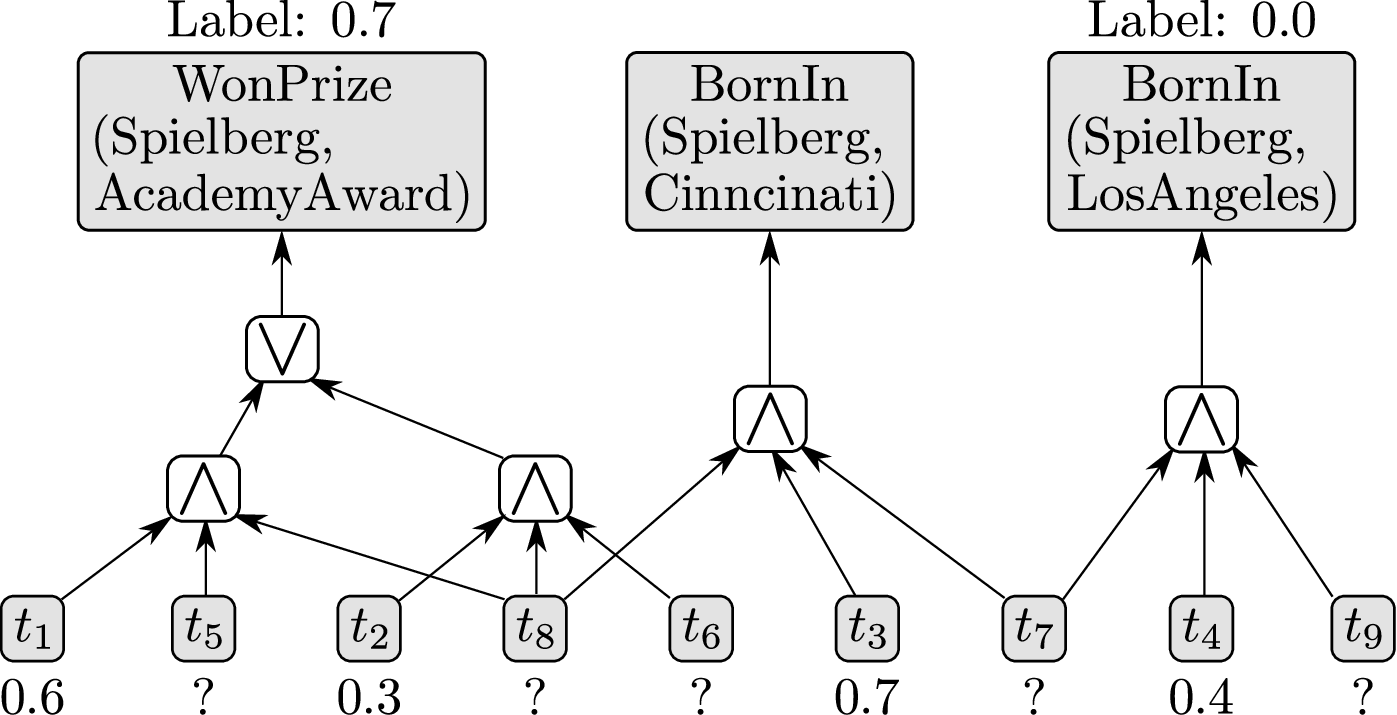
Refer to caption — Figure 2: Example Lineages and Labels

A closer look at the new tuples reveals, however, that not all of them are correct. For instance, BornIn(Spielberg,LosAngeles) is wrong, so we label it with the probability of $0.0$ . Moreover, WonPrize(Spielberg,AcademyAward) is likely correct, hence we label it with the probability of $0.7$ , as shown on top of Figure 2. Given the probability labels of the query answers, the goal of the learning procedure is to learn the base tuples’ unknown probability values for UsingPattern and FromDomain (while leaving the ones for WonPrizeExtraction and BornInExtraction unchanged), such that the lineage formulas again produce the given probability labels.

Contributions. We summarize the contributions of this work as follows.

$\bullet$

To our knowledge, we present the first approach to tackle the problem of learning unknown (or missing) tuple probabilities from labeled lineage formulas in the context of PDBs. In Section 4, we formally define the learning problem and analyze its properties from a theoretical perspective.
$\bullet$

We formulate the learning problem as an optimization problem, devise two different objective functions for solving it, and discuss both in Section 5.
$\bullet$

In Section 6, we present a learning algorithm based on stochastic gradient descent, which scales to problem instances with hundreds of thousands of labels and millions of tuples to learn the probability values for (Section 8.5).
$\bullet$

In Section 7, we show that the learning problem supports prior probabilities of base tuples which can be incorporated to update and clean PDBs. Also, we demonstrate that the learning problem subsumes both learning from incomplete databases [35] and applying constraints to PDBs [27].
$\bullet$

Additionally, we perform an experimental evaluation on three different real world datasets as well as on synthetic data (see Figure 4(a)), where we compare our approach to various techniques based on SRL, reasoning in information extraction, and optimization (Section 8).

2 Related Work

In the following, we briefly review a number of related works from the areas of SRL and PDBs, which we believe are closest to our work.

Machine Learning. Many machine learning approaches have been applied to large scale data sets (see [3] for an overview). However, the scalable methods tend to not offer a declarative language (similar to deduction rules or constraints) in order to induce correlations among facts, as queries and lineage do in PDBs. In contrast, in the subfield of SRL [18], correlations between ground atoms (similar to base tuples in PDBs) are often induced by logical formulas (similar to lineage in PDBs). But in turn, these methods lack scalability. Markov Logic Networks (MLNs) [32] (and their learning techniques [28, 34]) are built on an open-world assumption, which instantiates all combinations of constants, often resulting in a blow-up incompatible to database-like instance sizes. Even a very efficient implementation of MLNs, Markov: TheBeast [33], does not meet the scalability required for databases (see Section 8.3). As opposed to MLNs, ProbLog [11] computes marginal probabilities while relying on SLD proofs, which makes it very similar to PDBs with their closed-world assumption and deductive grounding techniques. However, also its learning procedure [22] does not scale well to large datasets (see Section 8.3). Within the ProbLog framework, [21] proposes the most similar approach to ours, however lacking both a theoretical analysis and large scale experiments.

Probabilistic Databases. A number of PDB engines, including MystiQ [6], MayBMS [2], and Trio [4] have been released as open-source prototypes in recent years and found a wide recognition in the database community. Due to the hardness of computing probabilities for query answers, a main focus of these approaches lies in finding tractable subclasses of query plans [9, 10, 36] for which probability computations can be done in polynomial time. A recent trend towards scalable inference is compiling Boolean formulas into more succinct representation formalisms such as OBDDs [24]. [8, 24], for example, develop an entire lattice of algebras and compilation techniques over unions of conjunctive queries (UCQs) which admit for polynomial-time inference. MarkoViews [23] represent another step towards SRL, by introducing uncertain views, where probabilities depend on the input tuples, but—still—do not tackle the actual learning problem. Also, [37] circumvent the learning problem by enabling direct querying of Conditional Random Fields via a probabilistic database.

Creating Probabilistic Databases. There are very few works on the actual creation of PDBs. The authors of [35] induce a probabilistic database by estimating probabilities from a given incomplete database, a problem that is subsumed by our definition of the learning problem (see Section 7.4). Enforcing consistency constraints by conditioning the base tuples of a PDB [27] onto these constraints allows for altering the tuple probabilities. Since conditioning lacks support for non-Boolean or inconsistent constraints, we can show that our work also subsumes this problem, but not the other way round (see Section 7.2). Similarly, incorporating user feedback by means of probabilistic data integration, as in [26], focuses on consistent, Boolean-only labels.

Lineage & Polynomials. The theoretical analysis of our learning problem (Section 4) is based on computing marginal probabilities via polynomials. Similarly, the authors of [19] used semirings over polynomials to model provenance, where lineage is a special case. Also, Sum-Product Networks [31] investigates tractable graphical models by representing these as polynomial expressions with polynomially many terms.

3 Probabilistic Databases

In this section, we introduce our data model which follows the common possible-worlds semantics over tuple-independent probabilistic databases with lineage [36], which is closed and complete [4]. Throughout this section, we assume that the probabilities of all base tuples are known and fixed (i.e., even for $t_{5}$ – $t_{9}$ in Example 1). Later, in Section 4 we relax this view to address the learning problem.

Probabilistic Database. We define a tuple-independent probabilistic database [36] $(\mathcal{T},p)$ as a pair consisting of a finite set of base tuples $\mathcal{T}$ and a probability measure $p:\mathcal{T}\rightarrow[0,1]$ , which assigns a probability value $p(t)$ to each uncertain tuple $t\in\mathcal{T}$ . As in a regular database, we assume the set of tuples $\mathcal{T}$ to be partitioned into a set of extensional relations (see, e.g., WonPrizeExtraction, BornInExtraction, UsingPattern, and FromDomain in Example 1). The probability value $p(t)$ of a base tuple $t$ thus denotes the confidence in the existence of the tuple in the database, i.e., a higher value $p(t)$ denotes a higher confidence in $t$ being valid.

Possible Worlds. Assuming independence among all base tuples $\mathcal{T}$ , the probability $P(\mathcal{W},\mathcal{T})$ of a possible world $\mathcal{W}\subseteq\mathcal{T}$ is defined as follows.

\displaystyle P(\mathcal{W},\mathcal{T}):=\prod_{t\in\mathcal{W}}p(t)\prod_{t\in\mathcal{T}\backslash\mathcal{W}}(1-p(t))

(3)

In the absence of any constraints (compare to Subsection 7.2) that would restrict this set of possible worlds, any subset $\mathcal{W}$ of tuples in $\mathcal{T}$ forms a valid possible world (i.e., a possible instance) of the probabilistic database. Hence, there are exponentially many possible worlds.

Deduction Rules. To support query answering over a PDB, we employ deduction rules (see, e.g., Rules (1) and (2)), which we express in a Datalog-style notation. Syntactically, these deduction rules have the shape of a logical implication with exactly one positive head literal and a conjunction of both positive and negative literals in the body. Formally, the class of rules we support corresponds to safe, non-recursive Datalog programs, which also coincides with the core operations expressible in the Relational Algebra [1].

Definition 1

A deduction rule is a logical rule of the form

R(\bar{X})\leftarrow\bigwedge_{i=1,\dots,n}R_{i}(\bar{X}_{i})\land\bigwedge_{j=1,\dots,m}\neg R_{j}(\bar{X}_{j})~~\land\Phi(\bar{X}^{\prime})

where

1.

$R$ denotes the head literal’s intensional relation, whereas $R_{i}$ , $R_{j}$ may refer to both intensional or extensional relations;
2.

$n\geq 1$ , $m\geq 0$ , thus requiring at least one positive relational literal;
3.

$\bar{X}$ , $\bar{X}_{i}$ , $\bar{X}_{j}$ , and $\bar{X}^{\prime}$ denote tuples of variables and constants, where $\mathit{Var}(\bar{X}),\mathit{Var}(\bar{X}_{j}),\mathit{Var}(\bar{X}^{\prime})\subseteq\bigcup_{i}\mathit{Var}(\bar{X}_{i})$ ;
4.

$\Phi(\bar{X}^{\prime})$ is a conjunction of arithmetic predicates, such as “ $=$ ”, “ $\neq$ ”, and “ $<$ ”.

Lineage. We utilize data lineage to represent the logical dependencies between base tuples in $\mathcal{T}$ and tuples derived from the deduction rules (see Figure 2). In analogy to [36], we consider lineage as a Boolean formula. It relates each derived tuple (or “query answer”) with the base tuples $\mathcal{T}$ via the three Boolean connectives $\land$ , $\lor$ and $\neg$ , which reflect the semantics of the relational operations that were applied to derive that tuple. Specifically, we employ

$\bullet$

a conjunction ( $\land$ ) that connects the relational literals in the body of a deduction rule;
$\bullet$

a negation ( $\neg$ ) for a negated relational literal in the body of a deduction rule;
$\bullet$

a disjunction ( $\lor$ ) whenever the same tuple is obtained from the head literals of two or more deduction rules;
$\bullet$

a Boolean (random) variable $t$ representing a tuple in $\mathcal{T}$ whenever an extensional literal matches this tuple.

For a formal definition of lineage in combination with Datalog rules and relational operators, we refer the reader to [15] and [36], respectively.

Example 2

In Figure 2, the conjunctions ( $\land$ ) are obtained from instantiating the conjunctions in Rule (1) and (2)’s bodies. Because two instances of Rule (1) result in the same derived tuple WonPrize(Spielberg,AcademyAward), the disjunction ( $\lor$ ) connects the two instantiated bodies. $\diamond$

Marginal Probabilities. We say that a possible world $\mathcal{W}$ entails a Boolean lineage formula $\phi$ , denoted as $\mathcal{W}\models\phi$ , if it represents a satisfying truth assignment to $\phi$ by setting all tuples in $\mathcal{W}$ to true and all tuples in $\mathcal{T}\backslash\mathcal{W}$ to false. Then, we can compute the marginal probability of any Boolean formula $\phi$ over tuples in $\mathcal{T}$ as the sum of the probabilities of all the possible worlds $\mathcal{W}\subseteq\mathcal{T}$ that entail $\phi$ :

P(\phi):=\sum_{\mathcal{W}\subseteq\mathcal{T},\mathcal{W}\models\phi}~\underbrace{P(\mathcal{W},\mathcal{T})}_{\text{via Eq.}~\eqref{eq:ProbPossibleWorld}}

(4)

To avoid the exponential cost involved in following Equation (4), we can—in many cases—compute the marginal probability $P(\phi)$ directly on the structure of the lineage formula $\phi$ [36]. Let $T(\phi)\subseteq\mathcal{T}$ denote the set of base tuples occurring in $\phi$ .

\small\!\!\begin{array}[]{rcl|c}\lx@intercol\hfil\text{Definition}\hfil\lx@intercol\vrule\lx@intercol&\text{Condition}\\ \hline\cr P(t)&\!\!:=&\!\!p(t)&t\in\mathcal{T}\\ P(\bigwedge_{i}\phi_{i})&\!\!:=&\!\!\prod_{i}P(\phi_{i})&i\!\neq\!j\Rightarrow\mathit{T}(\phi_{i})\!\cap\!\mathit{T}(\phi_{j})\!=\!\emptyset\\ P(\bigvee_{i}\phi_{i})&\!\!:=&\!\!1-\prod_{i}(1-P(\phi_{i}))&i\!\neq\!j\Rightarrow\mathit{T}(\phi_{i})\!\cap\!\mathit{T}(\phi_{j})\!=\!\emptyset\\ P(\phi\lor\psi)&\!\!:=&\!\!P(\phi)+P(\psi)&\phi\land\psi\equiv\mathit{false}\\ P(\neg\phi)&\!\!:=&\!\!1-P(\phi)&\\ \end{array}

(5)

The first line captures the case of a base tuple $t$ , for which we return its attached probability value $p(t)$ . The next two lines handle independent-and and independent-or operations for conjunctions and disjunctions over variable-disjoint subformulas $\phi_{i}$ , respectively. In the following line, we address disjunctions for two subformulas $\phi$ and $\psi$ that denote disjoint probabilistic events (known as disjoint-or [36]). The last line finally handles negation. Equation (5)’s definition of $P(\phi)$ runs in linear time in the size of $\phi$ . However, for general Boolean formulas, computing $P(\phi)$ is $\#\mathcal{P}$ -hard [9, 36]. This becomes evident if we consider Equation (6), called Shannon expansion, which is a form of variable elimination that is applicable to any Boolean formula:

P(\phi):=p(t)\cdot P(\phi_{[t\rightarrow\mathit{true}]})+(1-p(t))\cdot P(\phi_{[t\rightarrow\mathit{false}]})

(6)

Here, the notation $\phi_{[t\rightarrow\mathit{true}]}$ for a tuple $t\in T(\phi)$ denotes that we replace all occurrences of $t$ in $\phi$ by true (and false, respectively). Repeated applications of Shannon expansions may however result in an exponential increase of $\phi$ . The hardness of computing $P(\phi)$ for general propositional formulas has been addressed by various techniques [36], such as knowledge compilation [24] or approximation [30].

Example 3

Consider $P((t_{1}\land t_{5}\land t_{8})\lor(t_{2}\land t_{6}\land t_{8}))$ and assume $p(t_{5})=0.5$ , $p(t_{6})=0.6$ , and $p(t_{8})=0.8$ in addition to the known tuple probabilities shown in Figure 1. First, Line 3 of Equation (5) is not applicable, since $t_{8}$ occurs on both sides. So we apply a Shannon expansion, yielding $p(t_{8})\cdot P((t_{1}\land t_{5})\lor(t_{2}\land t_{6}))+(1-p(t_{8}))\cdot P(\mathit{false})=0.8\cdot P((t_{1}\land t_{5})\lor(t_{2}\land t_{6}))$ , where we used $P(\mathit{false})=0.0$ . Next, we apply Line 3 of Equation (5) which results in $0.8\cdot(1-(1-P(t_{1}\land t_{5}))\cdot(1-P(t_{2}\land t_{6})))$ . Then, two applications of Line 2 deliver $0.8\cdot(1-(1-p(t_{1})\cdot p(t_{5}))\cdot(1-p(t_{2})\cdot p(t_{6})))$ which can be simplified to $0.3408$ . $\diamond$

Marginal Probabilities via Polynomials. For the theoretical analysis of the learning problem presented in Section 4, we next devise an alternative way of computing marginals via polynomial expressions. As a preliminary, we reduce the number of terms in Equation (4)’s sum by considering just tuples $T(\phi)$ that occur in $\phi$ [36].

Proposition 1

We can compute $P(\phi)$ relying on tuples in $T(\phi)$ , only, by writing:

P(\phi)=\sum_{V\subseteq T(\phi),V\models\phi}\underbrace{P(V,T(\phi))}_{\text{via Eq.}~\eqref{eq:ProbPossibleWorld}}

(7)

Equation (7) expresses $P(\phi)$ as a polynomial. Its terms are defined by Equation (3), and the variables are $p(t)$ for $t\in T(\phi)$ . The polynomial’s degree is limited as follows.

Corollary 1

A lineage formula $\phi$ ’s marginal probability $P(\phi)$ can be expressed by a multi-linear polynomial over variables $p(t)$ , for $t\in T(\phi)$ , with a degree of at most $|T(\phi)|$ .

Proof 3.1.

By inspecting Proposition 1, we note that the sum ranges over subsets of $T(\phi)$ only, hence each term has a degree of at most $|T(\phi)|$ .

Example 3.2.

Considering the lineage formula $\phi\equiv t_{1}\lor t_{2}$ , the occurring tuples are $T(\phi)=\{t_{1},t_{2}\}$ . Then, it holds that $\{t_{1},t_{2}\}\models\phi$ , $\{t_{1}\}\models\phi$ , and $\{t_{2}\}\models\phi$ . Hence, we can write $P(\phi)=p(t_{1})\cdot p(t_{2})+p(t_{1})\cdot(1-p(t_{2}))+(1-p(t_{1}))\cdot p(t_{2})$ . Thus, $P(\phi)$ is a polynomial over the variables $p(t_{1})$ , $p(t_{2})$ and has degree $2=|T(\phi)|=|\{t_{1},t_{2}\}|$ . $\diamond$

4 Learning Problem

We now move away from the case where the probability values of all base tuples are known. Instead, we intend to learn the unknown probability values of (some of) these tuples (e.g. of $t_{5}$ – $t_{9}$ in Example 1). More formally, for a tuple-independent probabilistic database $(\mathcal{T},p)$ , we consider $\mathcal{T}_{l}\subseteq\mathcal{T}$ to be the set of base tuples for which we learn their probability values. That is, initially $p(t)$ is unknown for all $t\in\mathcal{T}_{l}$ . Conversely, $p(t)$ is known and fixed for all $t\in\mathcal{T}\backslash\mathcal{T}_{l}$ . To be able to complete $p(t)$ , we are given labels in the form of pairs $(\phi_{i},l_{i})$ , each containing a lineage formula $\phi_{i}$ (i.e., a query answer) and its desired marginal probability $l_{i}$ . We formally define the resulting learning problem as follows.

Definition 4.3.

We are given a probabilistic database $(\mathcal{T},p)$ , a set of tuples $\mathcal{T}_{l}\subseteq\mathcal{T}$ with unknown probability values $p(t_{l})$ and a multi-set of given labels $\mathcal{L}=\langle(\phi_{1},l_{1}),\dots,$ $(\phi_{n},l_{n})\rangle$ , where each $\phi_{i}$ is a lineage formula over $\mathcal{T}$ and each $l_{i}\in[0,1]\subset\mathbb{R}$ is a marginal probability for $\phi_{i}$ . Then, the learning problem is defined as follows:

\begin{array}[]{l}\text{Determine:}~~p(t_{l})\in[0,1]\subset\mathbb{R}~\text{for all}~t_{l}\in\mathcal{T}_{l}\\ \text{such that:}~~~P(\phi_{i})=l_{i}~\text{for all}~(\phi_{i},l_{i})\in\mathcal{L}\\ \end{array}

Intuitively, we aim to set the probability values of the base tuples $t_{l}\in\mathcal{T}_{l}$ such that the labeled lineage formulas $\phi_{i}$ yield the marginal probability $l_{i}$ . We want to remark that probability values of tuples in $\mathcal{T}\backslash\mathcal{T}_{l}$ remain unaltered. Also, we note that the Boolean labels true and false can be represented as $l_{i}=0.0$ and $l_{i}=1.0$ , respectively. Hence, Boolean labels resolve to a special case of Definition 4.3’s labels.

Example 4.4.

Formalizing Example 1’s problem setting, we obtain $\mathcal{T}:=\{t_{1},\dots,t_{9}\}$ , $\mathcal{T}_{l}:=\{t_{5},\dots,t_{9}\}$ with labels $((t_{1}\land t_{5}\land t_{8})\lor(t_{2}\land t_{6}\land t_{8}),0.7)$ , and $((t_{3}\land t_{7}\land t_{9}),0.0)$ . $\diamond$

Unfortunately, the above problem definition exhibits hard instances. First, computing $P(\phi_{i})$ may be $\#\mathcal{P}$ -hard [9], which would require many Shannon expansions. But even for cases when all $P(\phi_{i})$ can be computed in polynomial time (i.e., when Equation (5) is applicable), there are combinatorially hard cases of the above learning problem.

Lemma 4.5.

For a given instance of Definition 4.3’s learning problem, where all $P(\phi_{i})$ with $(\phi_{i},l_{i})\in\mathcal{L}$ can be computed in polynomial time, deciding whether there exists a solution to the learning problem is $\mathcal{NP}$ -hard.

Proof 4.6.

We encode the 3-satisfiability problem (3SAT) for a Boolean formula $\Psi\equiv\psi_{1}\land\dots\land\psi_{n}$ in CNF into Definition 4.3’s learning problem. For each variable $X_{i}\in\mathit{Var}(\Psi)$ , we create two tuples $t_{i}$ , $t^{\prime}_{i}$ whose probability values will be learned. Hence, $2\cdot|\mathit{Var}(\Psi)|=|\mathcal{T}_{l}|=|\mathcal{T}|$ . Then, for each $X_{i}$ , we add the label $((t_{i}\land t^{\prime}_{i})\lor(\neg t_{i}\land\neg t^{\prime}_{i}),1.0)$ . The corresponding polynomial equation $p(t_{i})p(t^{\prime}_{i})+(1-p(t_{i}))(1-p(t^{\prime}_{i}))=1.0$ has exactly two possible solutions for $p(t_{i}),p(t^{\prime}_{i})\in[0,1]$ , namely $p(t_{i})=p(t^{\prime}_{i})=1.0$ and $p(t_{i})=p(t^{\prime}_{i})=0.0$ . Next, we replace all variables $X_{i}$ in $\Psi$ by their tuple $t_{i}$ . Now, for each clause $\psi_{i}$ of $\Psi$ , we introduce one label $(\psi_{i},1.0)$ . Altogether, we have $|\mathcal{L}|=|\mathit{Var}(\Psi)|+n$ labels for Definition 4.3’s problem. Each labeled lineage formula $\phi$ has at most three variables, hence $P(\phi)$ takes at most 8 steps. Still, Definition 4.3 solves 3SAT, where the learned values of each pair of $p(t_{i})$ , $p(t^{\prime}_{i})$ (either $0.0$ or $1.0$ ) correspond to $X_{i}$ ’s truth value for a satisfying assignment of $\Psi$ . From this, it follows that the decision problem formulated in Lemma 4.5 is $\mathcal{NP}$ -hard.

Besides computationally hard instances, there might also be inconsistent instances of the learning problem. That is, it may be impossible to define $p:\mathcal{T}_{l}\rightarrow[0,1]$ such that all labels are satisfied.

Example 4.7.

If we consider $\mathcal{T}_{l}:=\{t_{1},t_{2}\}$ with the labels $\mathcal{L}:=\langle(t_{1},0.2),(t_{2},0.3),(t_{1}\land t_{2},0.9)\rangle$ , then it is impossible to fulfill all three labels at the same time.

From a practical point of view, there remain a number of questions regarding Definition 4.3. First, how many labels do we need in comparison to the number of tuples for which we are learning the probability values (i.e., $|\mathcal{L}|$ vs. $|\mathcal{T}_{l}|$ )? And second, is there a difference in labeling lineage formulas that involve many tuples or very few tuples (i.e., $|T(\phi_{i})|$ )? These questions will be answered by the following theorem. It is based on Corollary 1’s computation of marginal probabilities via their polynomial representation. We write the learning problem’s conditions $P(\phi_{i})=l_{i}$ as polynomials over variables $p(t_{l})$ of the form $P(\phi_{i})-l_{i}$ , where $t_{l}\in\mathcal{T}_{l}$ and the probability values $p(t)$ for all $t\in\mathcal{T}\backslash\mathcal{T}_{l}$ are fixed and hence represent constants.

Theorem 4.8.

If the labeling is consistent, Definition 4.3’s problem instances can be classified as follows:

1.

If $|\mathcal{L}|<|\mathcal{T}_{l}|$ , the problem has infinitely many solutions.
2.

If $|\mathcal{L}|=|\mathcal{T}_{l}|$ and the polynomials $P(\phi_{i})-l_{i}$ have common zeros, then the problem has infinitely many solutions.
3.

If $|\mathcal{L}|=|\mathcal{T}_{l}|$ and the polynomials $P(\phi_{i})-l_{i}$ have no common zeros, then the problem has at most $\prod_{i}|T(\phi_{i})\cap\mathcal{T}_{l}|$ solutions.
4.

If $|\mathcal{L}|>|\mathcal{T}_{l}|$ , then the polynomials $P(\phi_{i})-l_{i}$ have common zeros, thus reducing this to one of the previous cases.

Proof 4.9.

The first case is a classical under-determined system of equations. In the second case, without loss of generality, there are two polynomials $P(\phi_{i})-l_{i}$ and $P(\phi_{j})-l_{j}$ with a common zero, say $p(t_{k})=c_{k}$ . Setting $p(t_{k})=c_{k}$ satisfies both $P(\phi_{i})-l_{i}=0$ and $P(\phi_{j})-l_{j}=0$ , hence we have $\mathcal{L}^{\prime}:=\mathcal{L}\backslash\langle(\phi_{i},l_{i}),(\phi_{j},l_{j})\rangle$ and $\mathcal{T}^{\prime}_{l}:=\mathcal{T}_{l}\backslash\{t_{k}\}$ which yields the theorem’s first case again ( $|\mathcal{L}^{\prime}|<|\mathcal{T}^{\prime}_{l}|$ ). Regarding the third case, Bezout’s theorem [12], a central result from algebraic geometry, is applicable: for a system of polynomial equations, the number of solutions (including their multiplicities) over variables in $\mathbb{C}$ is equal to the product of the degrees of the polynomials. In our case, the polynomials are $P(\phi_{i})-l_{i}$ with variables $p(t_{l}),t_{l}\in\mathcal{T}_{l}$ . So, according to Corollary 1 their degree is at most $|T(\phi_{i})\cap\mathcal{T}_{l}|$ . Since our variables $p(t_{l})$ range only over $[0,1]\subset\mathbb{R}$ , and Corollary 1 is an upper bound only, $\prod_{i}|T(\phi_{i})\cap\mathcal{T}_{l}|$ is an upper bound on the number of solutions. In the fourth case, the system of equations is over-determined, such that redundancies like common zeros will reduce the problem to one of the previous cases.

Example 4.10.

We illustrate the theorem by providing examples for each of the four cases.

1.

In Example 4.4’s formalization of Example 1, we have $|\mathcal{T}_{l}|=5$ and $|\mathcal{L}|=2$ . So, the problem is under-specified and has infinitely many solutions, since assigning $p(t_{7})=0.0$ enables $p(t_{9})$ to take any value in $[0,1]\subset\mathbb{R}$ .
2.

We assume $\mathcal{T}_{l}=\{t_{5},t_{6},t_{7}\}$ , and $\mathcal{L}=\langle(t_{5}\land\neg t_{6},0.0),(t_{5}\land\neg t_{6}\land t_{7},0.0),(t_{5}\land t_{7},0.0)\rangle$ . This results in the equations $p(t_{5})\cdot(1-p(t_{6}))=0.0$ , $p(t_{5})\cdot(1-p(t_{6}))\cdot p(t_{7})=0.0$ , and $p(t_{5})\cdot p(t_{7})=0.0$ , where $p(t_{5})$ is a common zero to all three polynomials. Hence, setting $p(t_{5})=0.0$ allows $p(t_{6})$ and $p(t_{7})$ to take any value in $[0,1]\subset\mathbb{R}$ .
3.
Let us consider $\mathcal{T}_{l}=\{t_{7},t_{8}\}$ .
- (a)
  
  If $\mathcal{L}=\langle(t_{7},0.4),(t_{8},0.7)\rangle$ , then there is exactly one solution as predicted by $|T(t_{7})|\cdot|T(t_{8})|=1$ .
- (b)
  
  If $\mathcal{L}=\langle(t_{7}\land t_{8},0.1),(t_{7}\lor t_{8},0.6)\rangle$ , then there are two solutions, namely $p(t_{7})=0.2$ , $p(t_{8})=0.5$ and $p(t_{7})=0.5$ , $p(t_{8})=0.2$ . Here, $\prod_{i}|T(\phi_{i})\cap\mathcal{T}_{l}|=|T(t_{7}\land t_{8})|\cdot|T(t_{7}\lor t_{8})|=4$ is an upper bound.
4.

We extend this example’s second case by the label $(t_{5},0.0)$ , thus yielding the same solutions but having $|\mathcal{L}|>|\mathcal{T}_{l}|$ . $\diamond$

In general, a learning problem instance has many solutions, where Definition 4.3 does not specify a precedence, but all of them are equivalent. The number of solutions shrinks by adding labels to $\mathcal{L}$ , or by labeling lineage formulas $\phi_{i}$ that involve fewer tuples in $\mathcal{T}_{l}$ (thus resulting in a smaller intersection $|T(\phi_{i})\cap\mathcal{T}_{l}|$ ). Hence, to achieve more uniquely specified probabilities for all tuples $t_{l}\in\mathcal{T}_{l}$ , in practice we should obtain the same number of labels as the number of tuples for which we learn their probability values, i.e., $|\mathcal{L}|=|\mathcal{T}_{l}|$ , and label those lineage formulas with fewer tuples in $\mathcal{T}_{l}$ .

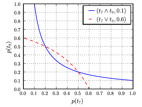
Based on algebraic geometry, the learning problem allows for an interesting visual interpretation. All possible definitions of probability values for tuples in $\mathcal{T}_{l}$ , that is $p:\mathcal{T}_{l}\rightarrow[0,1]$ , span the hypercube $[0,1]^{|\mathcal{T}_{l}|}$ . In Example 4.10, Cases 3(a) and 3(b), the hypercube has two dimensions, namely $p(t_{7})$ and $p(t_{8})$ , as depicted in Figures 3(a) and 3(b). Hence, one definition of $p$ specifies exactly one point in the hypercube. Moreover, all definitions of $p$ that satisfy a given label define a curve (or plane) through the hypercube (e.g., the two labels in Figure 3(a) define two straight lines). Also, the points, in which all labels’ curves intersect, represent solutions to the learning problem (e.g., the solutions of Example 4.10, Case 3(b), are the intersections in Figure 3(b)). If the learning problem is inconsistent, there is no point in which all labels’ curves intersect. Furthermore, if the learning problem has infinitely many solutions, the labels’ curves intersect in curves or planes, rather than points.

5 Solving the Learning Problem

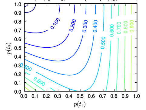
In the previous section, we formally characterized the learning problem and devised the basic properties of its solutions. From a visual perspective, Definition 4.3 established curves and planes whose intersections represent the solutions (see, e.g., Figure 3(b)). In this section, we introduce different objective functions that describe surfaces whose optima correspond to these solutions. For instance, Figure 3(b)’s problem has Figure 3(c)’s surface if we the use mean squared error (MSE) as the objective, which will be defined in this section. Calculating a gradient on such a surface thus allows the application of an optimization method to solve the learning problem.

Alternative Approaches. In general, based on the polynomial equations, an exact solution to an instance of the learning problem can be computed in exponential time [12], which is not acceptable in a database setting. Also, besides gradient-based optimization methods, other approaches, such as expectation maximization [20], are possible and represent valuable targets for future work.

Derivative. In order to establish a gradient on Definition 4.3’s conditions, i.e., $P(\phi_{i})=l_{i}$ , we introduce the partial derivative of a lineage formula’s marginal probability $P(\phi)$ with respect to a given tuple $t\in T(\phi)$ .

Definition 5.11.

[25] Given a lineage formula $\phi$ and a tuple $t\in T(\phi)$ , the partial derivative of $P(\phi)$ with respect to $p(t)$ is defined as:

\frac{\partial P(\phi)}{\partial p(t)}:=P(\phi_{[t\rightarrow\mathit{true}]})-P(\phi_{[t\rightarrow\mathit{false}]})

Here, $\phi_{[t\rightarrow\mathit{true}]}$ means that all occurrences of $t$ in $\phi$ are replaced by true (and analogously for false).

Example 5.12.

Considering the marginal probability $P(t_{1}\lor t_{2})$ with $p(t_{1})=0.6$ , we determine the partial derivative with respect to $p(t_{2})$ , that is $\frac{\partial P(t_{1}\lor t_{2})}{\partial p(t_{2})}=P(t_{1}\lor\mathit{true})-P(t_{1}\lor\mathit{false})=1.0-0.6=0.4$ . $\diamond$

Desired Properties. Before we define objective functions for solving the learning problem, we establish a list of desired properties of these (which we do not claim to be complete). Later, we judge different objectives based on these properties.

Definition 5.13.

An objective function to the learning problem should satisfy the following three desired properties:

1.

All instances of Definition 4.3’s learning problem can be expressed, including inconsistent ones.
2.

If all $P(\phi_{i})$ are computable in polynomial time, then also the objective is computable in polynomial time.
3.

The objective is stable, that is $\mathcal{L}:=\langle(\phi_{1},l_{1}),\dots,$ $(\phi_{n},l_{n})\rangle$ and $\mathcal{L}\cup\langle(\phi_{i}^{\prime},l_{i})\rangle$ with $\phi_{i}^{\prime}\equiv\phi_{i}$ , $(\phi_{i},l_{i})\in\mathcal{L}$ define the same surface.

Here, the first case ensures that the objective can be applied to all instances of the learning problem. We insist on inconsistent instances, because they occur often in practice (see Figure 4(a)). The second property restricts a blow-up in computation, which yields the following useful characteristic: if we can compute $P(\phi)$ for all labels, e.g., for labeled query answers, then we can also compute the objective function. Finally, the last of the desiderata reflects an objective function’s ability to detect dependencies between labels. Since $\phi_{i}\equiv\phi_{i}^{\prime}$ both $\mathcal{L}$ and $\mathcal{L}\cup\langle(\phi_{i}^{\prime},l_{i})\rangle$ allow exactly the same solutions, the surface should be the same. Unfortunately, including convexity of an objective as an additional desired property is not possible. For example Figure 3(b) has two disconnected solutions, which induce at least two optima, thus prohibiting convexity. In the following, we establish two objective functions, which behave very differently with respect to the desired properties.

Logical Objective. If we restrict the learning problem’s probability labels to $l_{i}\in\{0.0,1.0\}$ , we can define a objective function based on computing marginals as follows.

Definition 5.14.

Let an instance of Definition 4.3’s learning problem be given by a probabilistic database $(\mathcal{T},p)$ , tuples with unknown probability values $\mathcal{T}_{l}\subseteq\mathcal{T}$ , and labels $\mathcal{L}=\langle(\phi_{1},l_{1}),\dots,$ $(\phi_{n},l_{n})\rangle$ such that all $l_{i}\in\{0.0,1.0\}$ . Then, the logical objective is formulated as:

\mathit{Logical}(\mathcal{L},p):=P\left(\bigwedge_{(\phi_{i},l_{i})\in\mathcal{L},l_{i}=1.0}\!\!\!\!\!\!\phi_{i}~\land\bigwedge_{(\phi_{i},l_{i})\in\mathcal{L},l_{i}=0.0}\!\!\!\!\!\!\!\!\!\!\neg\phi_{i}\right)

(8)

The above definition is a maximization problem, and its global optima are identified by $\mathit{Logical}(\mathcal{L},p)=1.0$ . Moreover, from Definition 5.11, we may obtain its derivative.

Example 5.15.

Let $\mathcal{T}=\mathcal{T}_{l}:=\{t_{1},t_{2}\}$ and $\mathcal{L}:=\langle(t_{1}\lor t_{2},1.0),(t_{1},0.0)\rangle$ be given. Then, $\mathit{Logical}(\mathcal{L},p)$ is instantiated as $P((t_{1}\lor t_{2})\land\neg t_{1})=P(\neg t_{1}\land t_{2})$ . Visually, this defines a surface whose optimum lies in $p(t_{1})=0.0$ and $p(t_{2})=1.0$ , as shown in Figure 3(d). $\diamond$

With respect to Definition 5.13, the third desired property is fulfilled, as $P(\phi_{i}^{\prime}\land\phi_{i})=P(\phi_{i})$ . Hence, the logical objective’s surface, shown for instance in Figure 3(d), is never altered by adding equivalent labels. Still, the first property is not given, since the probability labels are restricted to $l_{i}\in\{0.0,1.0\}$ and inconsistent problem instances collapse Equation (8) to $P(\mathit{false})$ , thus rendering the objective non-applicable. Also, the second property is violated, because in the spirit of Lemma 4.5’s proof, we can construct an instance where each label’s $P(\phi_{i})$ on its own is computable in polynomial time, whereas the computation of the marginal probability for Equation (8) is $\mathcal{\#P}$ -hard.

Mean Squared Error Objective. Another approach, which is common in machine learning, lies in using the mean squared error (MSE) to define the objective function.

Definition 5.16.

Let an instance of Definition 4.3’s learning problem be given by a probabilistic database $(\mathcal{T},p)$ , tuples with unknown probability values $\mathcal{T}_{l}\subseteq\mathcal{T}$ , and labels $\mathcal{L}=\langle(\phi_{1},l_{1}),\dots,$ $(\phi_{n},l_{n})\rangle$ . Then, the mean squared error objective function is formulated as:

\mathit{MSE}(\mathcal{L},p):=\frac{1}{|\mathcal{L}|}\sum_{(\phi_{i},l_{i})\in\mathcal{L}}(P(\phi_{i})-l_{i})^{2}

Moreover, its partial derivative with respect to the tuple’s probability value $p(t)$ is:

\frac{\partial\mathit{MSE}(\mathcal{L},p)}{\partial p(t)}:=\frac{1}{|\mathcal{L}|}\sum_{(\phi_{i},l_{i})\in\mathcal{L},t\in T(\phi_{i})}\!\!\!\!\!2\cdot(P(\phi_{i})-l_{i})\cdot\underbrace{\frac{\partial P(\phi_{i})}{\partial p(t)}}_{\text{Def.}~\ref{def:confDerivative}}

The above formulation is a minimization problem whose solutions have $0.0$ as the objective’s value.

Example 5.17.

Example 4.10, Case 3(b), is visualized in Figure 3(b). The corresponding surface induced by the MSE objective is depicted in Figure 3(c) and has its minima at the learning problem’s solutions. $\diamond$

Judging the above objective by means of Definition 5.13, we realize that the first property is met, as there are no restrictions on the learning problem, and inconsistent instances can be tackled (but deliver objective values larger than zero). Furthermore, since the $P(\phi_{i})$ ’s occur in separate terms of the objective’s sum, the second desired property is maintained. However, the third desired property is violated, as illustrated by the following example.

Example 5.18.

In accordance to Example 5.15 and Figure 3(d), we set $\mathcal{T}=\mathcal{T}_{l}:=\{t_{1},t_{2}\}$ and $\mathcal{L}:=\langle(t_{1}\lor t_{2},1.0),$ $(t_{1},0.0)\rangle$ . Then, the MSE objective defines the surface in Figure 3(e). However, if we replicate the label $(t_{1},0.0)$ , thus resulting in Figure 3(f) (note the “times two” in the objective), its surface becomes steeper along the $p(t_{1})$ -axis, but has the same minimum. Thus, MSE’s surface is not stable. Instead, it becomes more ill-conditioned [29]. $\diamond$

Discussion. Both the logical objective and the MSE objective have optima exactly at the solutions of Definition 4.3’s learning problem. With respect to Definition 5.13’s desired properties, we summarize the behavior of both objectives in the following table:

\begin{array}[]{r|c|c|c}&\lx@intercol\hfil\text{Properties}\hfil\lx@intercol\\ \text{Objective}&1.&2.&3.\\ \hline\cr\text{Logical}&\times&\times&\checkmark\\ \text{MSE}&\checkmark&\checkmark&\times\\ \end{array}

The two objectives satisfy opposing desired properties, and it is certainly possible to define other objectives behaving similarly to one of them. Unfortunately, there is little hope for an objective that is adhering to all three properties. The second property inhibits computational hardness. However, Lemma 4.5 and the third property’s logical tautology checking (i.e., $\models\phi_{i}\leftrightarrow\phi_{i}^{\prime}$ , which is co- $\mathcal{NP}$ -complete) require these. In this regard the logical objective addresses both computationally hard problems by computing marginals, whereas the MSE objective avoids them.

In the remainder of the paper, we will favor the MSE objective, as it is more practical. In reality, many learning problem instances are inconsistent or have non-Boolean labels (see Figure 4(a)), and Equation (8)’s marginal computations are often too expensive (see Section 8.6).

6 Learning Algorithm

Given a learning problem’s surface (see, e.g., Figure 3(c)), as it is defined by the choice of the objective function, this section’s learning algorithm determines how to move over this surface in order to reach an optimum, that is, to find a solution to the learning problem.

Learning Algorithm. Our learning algorithm is based on stochastic gradient descend (SGD) [5], which we demonstrate to scale to instance sizes with millions of tuples and hundreds of thousands of labels (see Section 8.5). It is initialized at a random point and repeatedly moves into the direction of a partial derivative until convergence. Visually, we start at a random point (e.g., somewhere in Figure 3(c)), and then in each step we move in parallel to an axis (e.g., $p(t_{1})$ or $p(t_{2})$ ), until we reach an optimum.

In Algorithm 1 $\mathit{best}$ , represents the objective’s best known value, where $p$ holds the corresponding probability values of tuples in $\mathcal{T}_{l}$ . Also, $\eta_{l}$ is the learning rate, which exists and may differ for each tuple in $\mathcal{T}_{l}$ . Line 6’s loop is executed until convergence to the absolute error bound of $\epsilon_{\mathit{abs}}$ . Then, Line 7 shuffles the order of $\mathcal{T}_{l}$ ’s tuples for the inner loop of Line 8. Within each iteration, Line 10 updates one tuple’s probability value, which yields the updated definition $p^{\prime}$ of $p$ . If $p^{\prime}$ is an improvement over $p$ with respect to the objective (as verified in Line 13), we assign $p^{\prime}$ to $p$ and double the tuple’s learning rate $\eta_{l}$ . Otherwise, $p^{\prime}$ is discarded, and the learning rate $\eta_{l}$ is halved.

Algorithm 1 Learning(

(\mathcal{T},p),\mathcal{T}_{l},\mathcal{L},\epsilon_{\mathit{abs}}

)

1: Probabilistic database

(\mathcal{T},p)

, tuples

\mathcal{T}_{l}

to learn the probability values for, labeled lineage formulas

\mathcal{L}

, error bound

\epsilon_{\mathit{abs}}

p

with learned probability values,

\mathit{best}

value of objective

\forall t_{l}\in\mathcal{T}_{l}:p(t_{l}):=\mathit{Rand}(0,1)

\triangleright

Random initialization

\forall t_{l}\in\mathcal{T}_{l}:\eta_{l}:=1.0

\triangleright

Per-tuple learning rate

\mathit{best}:=\mathit{MSE}(\mathcal{L},p)

\triangleright

Definition 5.16

6: while

\mathit{best}>\epsilon_{\mathit{abs}}

\mathit{sequence}:=\mathit{Shuffle}(\mathcal{T}_{l})

\triangleright

Permuted sequence

8: while

\neg\mathit{IsEmpty}(\mathit{sequence})

t_{l}:=\mathit{Pop}(\mathit{sequence})

\triangleright

Get first element

10:

p^{\prime}(t_{l}):=p(t_{l})-\eta_{l}\cdot\frac{\partial\mathit{MSE}(\mathcal{L},p)}{\partial p(t_{l})}

\triangleright

Definition 5.16

11:

p^{\prime}:=p\cup\{p^{\prime}(t_{l})\}

12:

\mathit{newVal}:=\mathit{MSE}(\mathcal{L},p^{\prime})

\triangleright

Definition 5.16

13: if

\mathit{newVal}<\mathit{best}

then

14:

\eta_{l}:=2\cdot\eta_{l}

\triangleright

Increase

t_{l}

’s learning rate

15:

p:=p^{\prime}

\triangleright

Keep new value of

p(t_{l})

16:

\mathit{best}:=\mathit{newVal}

17: else

18:

\eta_{l}:=\frac{1}{2}\cdot\eta_{l}

\triangleright

Decrease

t_{l}

’s learning rate

19: return

p

\mathit{best}

Example 6.19.

We execute Algorithm 1 on Figure 3(e)’s example. Following Definition 5.16 the corresponding partial derivatives are:

\begin{array}[]{rl}\frac{\partial\mathit{MSE}}{\partial p(t_{1})}:=&\!\!\!\!(P(t_{1}\lor t_{2})-1.0)\cdot(P(\mathit{true}\lor t_{2})-P(\mathit{false}\lor t_{2}))\\ &\!\!\!\!+(P(t_{1})-0.0)\cdot(P(\mathit{true})-P(\mathit{false}))\\ \frac{\partial\mathit{MSE}}{\partial p(t_{2})}:=&\!\!\!\!(P(t_{1}\lor t_{2})-1.0)\cdot(P(t_{1}\lor\mathit{true})-P(t_{1}\lor\mathit{false}))\\ \end{array}

(9)

Assuming that Line 3 delivers $p(t_{1})=0.7$ and $p(t_{2})=0.5$ , we get $\mathrm{best}=(-0.15)^{2}+(0.7)^{2}\approx 0.512$ in Line 5. If $\epsilon_{\mathit{abs}}=0.01$ we enter Line 6’s loop, where Line 7 randomly orders $t_{2}$ before $t_{1}$ . Then, $p(t_{2})$ ’s partial derivative evaluates as follows $\frac{\partial\mathit{MSE}}{\partial p(t_{2})}\big|_{(0.7,0.5)}=(0.85-1.0)\cdot(1.0-0.7)=-0.055$ . Since $\eta_{2}=1.0$ , we get $p^{\prime}(t_{2})=0.5-(-0.055)=0.555$ in Line 10. Hence, in Line 12, $\mathrm{newVal}=(-0.1335)^{2}+0.7^{2}\approx 0.508$ . As $0.508<0.512$ , Line 13’s condition turns true, such that we get $\eta_{2}=2.0$ , $p(t_{1})=0.7$ , $p(t_{2})=0.555$ and $\mathrm{best}=0.508$ . Hence, in further iterations the increased $\eta_{2}$ speeds up movements along $p(t_{2})$ ’s partial derivative. $\diamond$

Tackling MSE’s Instability. The disadvantage of the MSE objective is that it does not satisfy Definition 5.13’s third desired property. We argue, that Algorithm 1 counters to some extent the instability, which we illustrate by the following example.

Example 6.20.

Let us evaluate the gradient of Figures 3(e) and 3(f) in the point $p(t_{1})=p(t_{2})=0.5$ . Following Equation (9), we obtain the gradient $(0.375,-0.125)$ for Figure 3(e). Analogously, Figure 3(f) has $(0.875,-0.125)$ . Even although both figures show the same minimum, the gradients differ heavily in $p(t_{1})$ ’s partial derivative. $\diamond$

Inspecting the above example, we note that the gradient is indeed affected, but each partial derivative on its own points into the correct direction, i.e. increasing $p(t_{2})$ and decreasing $p(t_{1})$ . Hence, weighting the partial derivatives can counter the effect. We achieve this by keeping one learning rate $\eta_{l}$ per tuple and adapting them during runtime. In Section 8.4, we empirically show a superior convergence over a global learning rate. Previously, the authors of [28] also reported speed ups in ill-conditioned instances by introducing separate learning rates per dimension.

Implementation Issues. In this paragraph, we briefly describe four implementation issues, which were omitted in Algorithm 1 for presentation purposes. First, Line 6’s absolute error bound is inconvenient, because the optima of inconsistent learning problem instances have an MSE value larger than $0.0$ . Therefore, we use both an absolute error bound $\epsilon_{\mathit{abs}}$ and a relative error bound $\epsilon_{\mathit{rel}}$ . Second, since their marginal probabilities $P(\phi_{i})$ are repeatedly computed, it is beneficial to preprocess the lineage formulas $\phi_{i}$ , e.g. by compiling them to OBDDs [24], or by flattening them via a few targeted Shannon expansions [14], the latter of which we also apply in this work. Next, Line 10 might yield a probability value that exceeds the interval $[0,1]$ , which we counter by the logit function. It defines a mapping from probability values in $[0,1]$ to $\mathbb{R}\cup\{\pm\infty\}$ .

Definition 6.21.

The logit function transforms a probability $p\in[0,1]$ to a weight $w\in\mathbb{R}\cup\{\pm\infty\}$ as follows:

w=\ln\frac{p}{1.0-p}\hskip 20.00003ptp=\frac{1}{1+\exp(-w)}

Example 6.22.

If $p=0.5$ , then $w=0.0$ . Also $p=1.0$ implies $w=+\infty$ , whereas $p=0.0$ yields $w=-\infty$ . $\diamond$

Hence, we calculate with weights in $\mathbb{R}\cup\{\pm\infty\}$ , rather than on probability values in $[0,1]$ . Finally, if two tuples $t_{l},t_{l}^{\prime}\in\mathcal{T}_{l}$ are disjoint with respect to the labels’ lineage formulas they occur in, that is $\{\phi_{i}~|~(\phi_{i},l_{i})\in\mathcal{L},t_{l}\in T(\phi_{i}),t_{l}^{\prime}\in T(\phi_{i})\}=\emptyset$ , then their probability values can be updated in parallel.

Alternative Approaches. Due to its various applications, there is an entire zoo of gradient-based optimization techniques [29]. Approaches, such as Newton’s method, which are based on the Hessian, do not to scale to database-like instance sizes. This disadvantage is circumvented by Quasi-Newton methods, for instance limited-memory Broyden-Fletcher-Goldfarb-Shanno (L-BFGS) [29], which estimates the Hessian. We empirically compare our approach to L-BFGS and plain gradient descent in Section 8.4.

Algorithm Properties. Algorithm 1 comes with three properties, which we share with alternative approaches we are aware of, including other gradient-based methods and expectation maximization [20]. First, the algorithm is non-deterministic, which is caused by Lines 3 and 7. Second, gradient-based optimization methods, including Algorithm 1, can get stuck in local optima, which is nevertheless hard to avoid in non-convex problems. In this regard, the non-determinism is a potential advantage, since restarting the algorithm will yield varying solutions, thus increasing the chance for finding a global optimum. Finally, the solutions returned by Algorithm 1 for the MSE objective are not exact, but rather very close to an optimum, which however can be controlled by the error bounds $\epsilon_{\mathit{rel}}$ and $\epsilon_{\mathit{abs}}$ . Due to space constraints, experiments on these aspects are available in the supplementary material¹.

7 Extensions & Applications

In this section, we briefly investigate how the learning problem can be extended by priors (Section 7.1), how it relates to conditioning PDBs via constraints (Section 7.2), how these constraints can be employed to update or clean PDBs (Section 7.3), and how it relates to handling incompleteness in databases (Section 7.4).

7.1 Priors

In order to explicitly incorporate preferences in the form of prior probabilities of base tuples $t_{l}\in\mathcal{T}_{l}$ into our learning objective (instead of just considering them to be “unknown”), we can extend Definition 5.16’s MSE objective as follows.

Definition 7.23.

Given a function $\mathit{prior}:\mathcal{T}_{l}\rightarrow[0,1]\subset\mathbb{R}$ , Definition 5.16’s MSE objective function can be extended to

\frac{c}{|\mathcal{L}|}\cdot\!\!\sum_{(\phi_{i},l_{i})\in\mathcal{L}}(P(\phi_{i})-l_{i})^{2}+\frac{1-c}{|\mathcal{T}_{l}|}\cdot\!\!\sum_{t_{l}\in\mathcal{T}_{l}}(P(t_{l})-\mathit{prior}(t_{l}))^{2}

where $c\in[0,1]$ is a constant.

Utilizing $c$ , we can control the trade-off between the impact of the lineage labels and the $prior$ function.

Expressiveness. Definition 7.23 is not more general than the original MSE objective. We can express priors in Definition 5.16 by creating a label $(t_{l},\mathit{prior}(t_{l}))$ for each tuple $t_{l}\in\mathcal{T}_{l}$ , which then produces $\sum_{t_{l}\in\mathcal{T}_{l}}(P(t_{l})-\mathit{prior}(t_{l}))^{2}$ also in Definition 5.16’s objective. The coefficients preceding the sums can be emulated by replicating labels in $\mathcal{L}$ . Thus, priors are a special case of lineage labels.

7.2 Constraints

Conditioning by Learning. Considering constraints in the form of propositional formulas over a probabilistic database’s tuples, we can encode each constraint $\phi_{i}$ with the label $(\phi_{i},1.0)$ into an instance of the learning problem.

Lemma 7.24.

Given a probabilistic database $(\mathcal{T},p)$ and constraints in the form of propositional formulas $\phi_{1},\dots,\phi_{n}$ over $\mathcal{T}$ , whose conjunction $\phi_{1}\land\dots\land\phi_{n}$ is satisfiable. Then, if we create a learning problem instance by setting $\mathcal{T}_{l}:=\mathcal{T}$ and $\mathcal{L}:=\langle(\phi_{1},1.0),\dots,(\phi_{n},1.0)\rangle$ , its solution $p^{\prime}$ conditions the probabilistic database $(\mathcal{T},p)$ with respect to $\phi_{1},\dots,\phi_{n}$ . Hence, for a propositional query $\psi$ over $(\mathcal{T},p^{\prime})$ it holds, that:

P(\psi~|~\phi_{1}\land\dots\land\phi_{n})=P(\psi)

Proof 7.25.

We observe that in the learning problem’s solution $p^{\prime}$ , we get $P(\phi_{1}\land\dots\land\phi_{n})=1.0$ . Moreover, over $(\mathcal{T},p^{\prime})$ , we can rewrite the marginal probability of a query answer $\psi$ as follows.

\begin{array}[]{rl}P(\psi)&\!\stackrel{{\scriptstyle\eqref{eq:lineageConf}}}{{=}}\sum_{\mathcal{W}\subseteq\mathcal{T},\mathcal{\models}\psi}P(\mathcal{W},\mathcal{T})\\ &=\sum_{\mathcal{W}\subseteq\mathcal{T},\mathcal{W}\models\psi,\mathcal{W}\models\phi_{1},\dots,\mathcal{W}\models\phi_{n}}P(\mathcal{W},\mathcal{T})\\ &=P(\psi\land\phi_{1}\land\dots\land\phi_{n})\\ \end{array}

By combining both equations, we obtain over $(\mathcal{T},p^{\prime})$ :

P(\psi~|~\phi_{1}\land\dots\land\phi_{n})=\frac{P(\psi\land\phi_{1}\land\dots\land\phi_{n})}{P(\phi_{1}\land\dots\land\phi_{n})}=\frac{P(\psi)}{1.0}=P(\psi)

Thus, the learning problem subsumes conditioning PDBs [27]. From a Bayesian perspective, the solution to the learning problem $p^{\prime}$ can be seen as posterior probabilities of the base tuples in $\mathcal{T}_{l}$ .

Learning by Conditioning. Following Definition 5.14’s logical objective, we can apply constraint-enforcing approaches to solve a subset of possible learning problem instances. The subset is characterized by instances with consistent labels, having $\mathcal{T}=\mathcal{T}_{l}$ , and by restricting the lineage labels to $l_{i}\in\{0.0,1.0\}$ . We create a single constraint in the form of Equation (8)’s conjunction, initially set all tuple confidences to $0.5$ , and solve the resulting conditioning problem [27].

7.3 Updating & Cleaning PDBs

Updating. If we are given an existing probabilistic database $(\mathcal{T},p)$ and knowledge in the form of labeled lineage formulas $\mathcal{L}:=\langle(\phi_{1},l_{1}),\dots,(\phi_{n},l_{n})\rangle$ , we can update the tuples’ probability values via the learning problem. We produce a new probabilistic database $(\mathcal{T},p^{\prime})$ , whose probability values $p^{\prime}$ are updated according to the information provided in $\mathcal{L}$ . To achieve this, we create a learning problem instance (whose solution is $p^{\prime}$ ) by using $\mathcal{L}$ , setting $\mathcal{T}_{l}:=\mathcal{T}$ and defining a prior $\mathit{prior}(t):=p(t)$ .

Cleaning. The new probability values $p^{\prime}$ allow for cleaning the probabilistic database as follows. If $p^{\prime}$ defines a tuple’s probability value to be $0.0$ , we can delete it from the database. Conversely, if $p^{\prime}$ yields $1.0$ for a tuple’s probability value, we can move it into a new, deterministic relation.

7.4 Incomplete Databases

A field that is related to PDBs are incomplete databases. Intuitively, in an incomplete database, some attributes values or entire tuples may be missing in the given database instance. A completion of an incomplete database can be seen as a possible world in a PDB—with a probability.

Missing Attribute Values. In [35], a PDB is derived from an incomplete database which exhibits missing attributes in some of its tuples. Their idea is to estimate the probability of a possible completion of an incomplete tuple from the complete part of the database. We show that this approach is an instance of the learning problem via the following reduction.

Let an incomplete database be given by a set of complete tuples $\mathcal{T}_{c}$ and a set of incomplete tuples $\mathcal{T}_{i}$ . We consider an incomplete tuple $R(\bar{a})\in\mathcal{T}_{i}$ of relation $R$ , where one or more attributes in $\bar{a}$ lack values, such that all possible completions are represented by $\bar{a}_{i}\supsetneq\bar{a}$ (assuming finite domains). Then, we create a new uncertain relation $R^{\prime}:=\{\bar{a}_{i}~|~\bar{a}_{i}\supsetneq\bar{a}\}$ and add one deduction rule per completion $\bar{a}_{i}$ :

R(\bar{a}_{i})\leftarrow R^{\prime}(\bar{a}_{i})\land\bigwedge_{j\neq i}\neg R^{\prime}(\bar{a}_{j})

The above rules allow at most one completion of $\bar{a}$ to be true within a possible world, so the resulting lineage formulas form a block-independent PDB [36]. Now, we create labels following [35]’s approach. For a subset of argument values $\bar{s}\subset\bar{a}$ , we count how often the complete tuples $\mathcal{T}_{c}$ feature the completion $\bar{a}_{i}$ , in symbols $I_{\bar{s}}(\bar{a}_{i}):=|\{R(\bar{a}^{\prime})\in\mathcal{T}_{c}~|~\bar{a}\cap\bar{a}^{\prime}=\bar{s},\bar{a}_{i}\backslash\bar{a}\subset\bar{a}^{\prime}\}|$ . Then, for each completion $\bar{a}_{i}$ , we generate the label $(R(\bar{a}_{i}),$ $\frac{I_{\bar{s}}(\bar{a}_{i})}{\sum_{j}I_{\bar{s}}(\bar{a}_{j})})$ . Besides these labels, the resulting learning problem instance uses the new relations $R^{\prime}$ ’s tuples in $\mathcal{T}_{l}$ .

Missing Tuples. Generally, any database instance can be seen as a finite subset of the crossproduct of its attributes’ domains. We now consider an incomplete database, whose (finite sets of) existing tuples and potentially missing tuples are $\mathcal{T}_{c}$ and $\mathcal{T}_{m}$ , respectively. Assume we intend to enforce logical formulas $\phi_{1},\dots,\phi_{n}$ over tuples $\mathcal{T}_{c}\cup\mathcal{T}_{m}$ , which could for example result from constraints or user feedback. We create a learning problem instance by setting $\mathcal{T}:=\mathcal{T}_{c}\cup\mathcal{T}_{m}$ , $\mathcal{T}_{l}:=\mathcal{T}_{m}$ and $\mathcal{L}:=\langle(\phi_{1},1.0),\dots,(\phi_{n},1.0)\rangle$ . Thus, a solution to the learning problem will complete $\mathcal{T}_{c}$ with (possibly uncertain) tuples from $\mathcal{T}_{m}$ , such that the logical formulas $\phi_{1},\dots,\phi_{n}$ are fulfilled.

8 Experiments

Our evaluation focuses on the following four aspects. First, we compare the quality of our approach to learning techniques in SRL (Section 8.1) and to constraint-based reasoning techniques applied in information extraction settings (Section 8.2). Second, we compare the runtime behavior of our algorithm to SRL methods (Section 8.3) and to other gradient-based optimization techniques (Section 8.4). Third, we explore the scalability of our method to large data sets (Section 8.5). Finally, in Section 8.6, we investigate the runtime behavior of the two objective functions defined in Section 5. Due to space constraints, additional experiments on varying $\epsilon_{\mathit{abs}}$ , $\epsilon_{\mathit{rel}}$ and Algorithm 1’s ability to find global optima are available in the supplementary material¹¹ 1 http://www.mpi-inf.mpg.de/~mdylla/learning.pdf.

Overview. As an overview, we present the basic characteristics of all learning problem instances in Figure 4(a), where Avg. $T(\phi)$ is calculated as $\frac{1}{|\mathcal{L}|}\sum_{(\phi_{i},l_{i})\in\mathcal{L}}|T(\phi_{i})|$ .

Setup. Our engine is implemented in Java. It employs a PostgreSQL 8.4 database backend for evaluating Datalog rules in a bottom-up manner and to instantiate lineage formulas. If not stated otherwise, PDB refers to Algorithm 1’s implementation with the MSE objective and a per-tuple learning rate. For checking convergence, we set $\epsilon_{\mathit{abs}}=10^{-6}$ and $\epsilon_{\mathit{rel}}=10^{-4}$ . We ran all experiments on an 8-core Intel Xeon 2.4GHz machine with 48 GB RAM, repeated each setting four times, and report the average of the last three runs. Whenever different programs compete, all of them run in single-threaded mode. All rules used in the experiments are provided in the supplementary material¹.

8.1 Quality Task: SRL Setting

Dataset. We use the openly available UW-CSE dataset²² 2 http://alchemy.cs.washington.edu/data/uw-cse/, which comprises a database describing the University of Washington’s computer science department via the following relations: AdvisedBy, CourseLevel, HasPosition, InPhase, Professor, ProjectMember, Publication, Student, TaughtBy, Ta (teaching assistant), and YearsInProgram. Moreover, the dataset is split into five sub-departments, and we consider this dataset’s relations to be deterministic.

Task. The goal is inspired by an experiment in [32], namely to predict the AdvisedBy relation from all input relations except Student and Professor. We train and test in a leave-one-out fashion by sub-department.

Rules. We automatically create 49 rules resembling all joins (including self-joins) between two relations (except student, professor, and AdvisedBy), having at least one argument of type person. Furthermore, we add one uncertain relation rules, containing one tuple for each of the 49 rules and include the corresponding tuple in the join, for example:

\mathit{AdvisedBy}(P_{1},P_{2})\leftarrow\left(\!\!\!\begin{array}[]{r}\mathit{Ta}(D,C,P_{1},T)\land\\ \mathit{TaughtBy}(D,C,P_{2},T)\land\\ \end{array}\!\!\!\mathit{Rules}(1)\right)\vskip-2.84526pt

The remaining rules are given in the supplementary material¹. We learn the probability values of the 49 tuples, hence classifying how well each rule predicts the $\mathit{AdvisedBy}$ relation.

Labels. Regarding labels, we used the 113 instances of AdvisedBy as positive labels, i.e., all their probability labels are $1.0$ . In addition, there are about 16,000 person-person pairs not contained in AdvisedBy. We randomly draw pairs from these as negative labels (with a probability label of $0.0$ ).

SRL Competitors. We compete with TheBeast [33], the fastest Markov Logic [32] implementation we are aware of. It uses an in-memory database and performs inference via Integer Linear Programming. We ran it on the same set of data and rules. Additionally, we ran the probabilistic Prolog engine ProbLog [22], but even on the reduced datasize of one sub-department it did not terminate after one hour.

Results. In Figure 4(b), we depict both the runtimes as well as the prediction quality in terms of the $F_{1}$ measure (the harmonic mean of precision and recall) for the $\mathit{AdvisedBy}$ relation. TheBeast is a straight line, since it allows only positive labels. For PDB, we started with all positive labels and added increasing numbers of negative labels.

Analysis. Regarding runtimes, PDB is consistently about 40 times faster than TheBeast. With respect to $F_{1}$ , adding more negative labels to PDB yields improvements until we saturate at the same level as TheBeast.

8.2 Quality Task: Information Extraction

Dataset. This dataset³³ 3 http://www.mpi-inf.mpg.de/yago-naga/pravda/ contains about 450,000 crawled web pages in the sports and celebrities domains, where about 12,500 textual patterns are used to extract facts.

Task. Following [38], we consider two different relations, namely WorksForClub in the sports domain and IsMarriedTo in the celebrities domain. Both relations contain facts with temporal annotations. The goal is to determine, for each textual pattern, whether it expresses a temporal begin, during or end event of one of the two relations, or none of them. For example, for WorksForClub, we could find that David Beckham joined Real Madrid in 2003 (begin), scored goals for them in 2005 (during), and left the club in 2007 (end).

PDB Setup. We model temporal data in the PDB according to [14]. Text occurrences of a potential fact are stored in the deterministic relation $\mathit{Occurrence}(\mathit{Pid},\mathit{E1},\mathit{E2},\mathit{Types},$ $\mathit{Begin},\mathit{End})$ , where Types holds the entities’ types and Begin, End contain integers encoding the limits of their occurrences’ time intervals. To encode the decision whether a pattern expresses a temporal begin, during, or end event, we instantiate three uncertain relations $\mathit{Begin}(\mathit{Pid})$ , $\mathit{During}(\mathit{Pid})$ , and $\mathit{End}(\mathit{Pid})$ , which each hold one entry per pattern and whose probability values we learn. Text occurrences of potential facts are connected to the patterns by six rules (see¹ for details) of the following kind

\begin{array}[]{l}\mathit{IsMarriedToBegin}(E_{1},E_{2},T_{1},T_{2})\\ ~~\leftarrow\mathit{Begin}(\mathit{Pid})\land\mathit{Occurrence}(\mathit{Pid},E_{1},E_{1},pp,T_{1},T_{2})\\ \end{array}\vskip-2.84526pt

where $pp$ stands for person-person type pair. To enforce that a textual pattern expresses at most one of begin, during, or end, we make them mutually exclusive via the rules

\begin{array}[]{rcl}\mathit{Constraint1}(\mathit{Pid})&\leftarrow&\mathit{Begin}(\mathit{Pid})\land\mathit{During}(\mathit{Pid})\\ \mathit{Constraint2}(\mathit{Pid})&\leftarrow&\mathit{Begin}(\mathit{Pid})\land\mathit{End}(\mathit{Pid})\\ \mathit{Constraint3}(\mathit{Pid})&\leftarrow&\mathit{During}(\mathit{Pid})\land\mathit{End}(\mathit{Pid})\\ \end{array}\vskip-2.84526pt

whose resulting lineage formulas we label with $0.0$ . Moreover, we use temporal precedence constraints by instantiating six rules of the form

\mathit{Constraint4}(E_{1},E_{2})\leftarrow\!\!\!\begin{array}[]{l}\mathit{IsMarriedToBegin}(E_{1},E_{2},T_{1},T_{2})\land\\ \mathit{IsMarriedToDuring}(E_{1},E_{2},T_{3},T_{4})\\ ~~~\land T_{3}<T_{2}\\ \end{array}\vskip-2.84526pt

and label their lineage with $0.0$ . Finally, we employ the 266 labels for textual patterns and the 341 labels for facts from the original work [38].

Competitor. The authors of [38] utilized a combination of Label Propagation and Integer Linear Programming to rate the textual patterns and to enforce temporal constraints.

Results. In Figure 4(c), we report our system’s (PDB) result along with the best result from [38] (PRAVDA). To evaluate precision, we sampled 100 facts per relation and event type and annotated them manually. Recall is the absolute number of facts obtained.

Analysis. For relations with a few, decisive textual patterns, PDB keeps up with precision, while slightly gaining in recall, probably due to the relaxation of constraints by the MSE objective. However, for worksForClub’s during relation, there is a vast number of relevant patterns, which puts Label Propagation’s undirected model in favor, whereas our directed model suffers in terms of recall.

8.3 Runtime Task: SRL Methods

Setup. To systematically verify scalability, we create synthetic data sets as follows. We fix $\mathcal{T}=\mathcal{T}_{l}$ to 100 tuples. Then, we instantiate a growing number of lineage formulas of the form $(t\land\neg t\land\neg t)\lor(t\land\neg t\land\neg t)$ , where all tuple identifiers are uniformly drawn from $\mathcal{T}_{l}$ , and negations exist with probability $0.5$ . Each formula’s probability label is randomly set to either $0.0$ or $1.0$ .

Competitors. Besides TheBeast [33], we compete with ProbLog [22], a probabilistic Prolog engine, whose grounding techniques and distribution semantics are closest to ours.

Results. For each value of $|\mathcal{L}|$ , we create five problem instances and depict their average runtime in Figure 4(d).

Analysis. PDB converges on average about 600 times faster than ProbLog and about 70 times faster than TheBeast.

8.4 Runtime Task: Gradient Methods

Setup. We employ the openly available YAGO2⁴⁴ 4 http://www.mpi-inf.mpg.de/yago-naga/yago/ knowledge base, which comprises about 110 relations. The task is to learn the probability values of tuples $\mathcal{T}_{l}$ in the LivesIn relation. Moreover, we label the following rule’s

\mathit{ToLabel}(L)\leftarrow\mathit{LivesIn}(P,L)\vskip-2.84526pt

lineage formulas with synthetic target probabilities. Since the rule’s projection on the first argument makes all lineage formulas $\phi$ disjoint with respect to their tuples $T(\phi)$ , the resulting learning problem instance is consistent. Hence, its global optima have a mean squared error (MSE) of $0.0$ .

Competitors. Algorithm 1 with per tuple learning rate (SGD Per-Tuple) competes with a single learning rate (SGD Single), with gradient descent (GD), and with L-BFGS [29], which approximates the Hessian with its second derivatives. All methods are initialized with the same learning rate.

Results. We plot the MSE against the runtime of the different methods in Figure 4(e).

Analysis. GD takes less time per iteration. Hence its curves drops faster in the beginning, but then stagnates. The two SGD variants behave similarly at first. Later on, the per-tuple learning rate yields constant improvements, whereas the single learning rate does not. L-BFGS, finally, improves slowly in comparison.

8.5 Runtime Task: Scalability

Dataset. As previously, we run on YAGO2⁴. For tuples in $\mathcal{T}\backslash\mathcal{T}_{l}$ , we use uniformly drawn synthetic probability values.

Labels. In order to create labels, we run queries on YAGO2 and label their answers’ lineage formulas with synthetic target probabilities (see¹ for details).

Results. Figure 4(f) contains the results of three large learning problem instances $P1$ to $P3$ , where Init is the time spent on instantiating the lineage formulas, and Algorithm 1 had multi-threading enabled.

Analysis. The Init time is determined by the number ( $|\mathcal{L}|$ ) and size (Avg. $T(\phi)$ ) of lineage formulas being instantiated. Algorithm 1 is faster on consistent instances ( $P3$ ). Its runtime is dominated by the number of labels per tuple $t_{l}\in\mathcal{T}_{l}$ .

8.6 Runtime Task: Objectives

Setup. As a last experiment, we run Algorithm 1 once with the Logical objective (see Definition 5.14) and once with the mean-squared-error (MSE) objective (see Definition 5.16). The synthetic data is created analogously to Section 8.3.

Results & Analysis. Already on tiny instances of up to 15 labels as in Figure 4(g), the Logical objective slows down significantly in comparison to MSE, due to the expensive marginal computations of Equation (8).

9 Conclusions

We introduced a novel method for learning tuple confidences in tuple-independent probabilistic databases. We analyzed the properties of this learning problem from a theoretical perspective, devised gradient-based solutions, investigated the relationship to other problems, and presented an implementation together with extensive experiments. For future work, we see numerous promising directions. Studying tractable subclasses of the learning problem or dropping the tuple-independence assumption would improve our theoretical understanding. Other valuable targets lie in the creation of a large, publicly available benchmark and the application of the learning problem to a broader range of related problems, e.g., inspired by the ones mentioned in Section 7.

References

[1] S. Abiteboul, R. Hull, and V. Vianu. Foundations of Databases. Addison-Wesley, 1995.
[2] L. Antova, T. Jansen, C. Koch, and D. Olteanu. Fast and simple relational processing of uncertain data. In ICDE, pages 983–992, 2008.
[3] R. Bekkerman, M. Bilenko, and J. Langford, editors. Scaling up machine learning. Cambridge U.P., 2011.
[4] O. Benjelloun, A. D. Sarma, A. Y. Halevy, M. Theobald, and J. Widom. Databases with uncertainty and lineage. PVLDB, 17(2):243–264, 2008.
[5] L. Bottou and O. Bousquet. The tradeoffs of large scale learning. In NIPS, pages 161–168, 2008.
[6] J. Boulos, N. N. Dalvi, B. Mandhani, S. Mathur, C. Ré, and D. Suciu. MYSTIQ: a system for finding more answers by using probabilities. In SIGMOD, pages 891–893, 2005.
[7] N. Dalvi, C. Ré, and D. Suciu. Probabilistic databases: diamonds in the dirt. Commun. ACM, 52(7):86–94, 2009.
[8] N. Dalvi, K. Schnaitter, and D. Suciu. Computing query probability with incidence algebras. In PODS, pages 203–214, 2010.
[9] N. Dalvi and D. Suciu. The dichotomy of conjunctive queries on probabilistic structures. In PODS, pages 293–302, 2007.
[10] N. Dalvi and D. Suciu. Efficient query evaluation on probabilistic databases. PVLDB, 16(4):523–544, 2007.
[11] L. De Raedt, A. Kimmig, and H. Toivonen. ProbLog: a probabilistic prolog and its application in link discovery. In IJCAI, pages 2468–2473, 2007.
[12] A. Dickenstein and I. Z. Emiris. Solving Polynomial Equations: Foundations, Algorithms, and Applications. Springer, 2005.
[13] M. Dylla. Efficient querying and learning in probabilistic and temporal databases. PhD thesis, Saarland University, 2014.
[14] M. Dylla, I. Miliaraki, and M. Theobald. A temporal-probabilistic database model for information extraction. PVLDB, 6(14), 2013.
[15] M. Dylla, I. Miliaraki, and M. Theobald. Top-k Query Processing in Probabilistic Databases with Non-Materialized Views. In ICDE, pages 122–133, 2013.
[16] M. Dylla and M. Theobald. Learning tuple probabilities in probabilistic databases. Research Report MPI-I-2014-5-001, Max-Planck-Institute Informatics, 2014.
[17] M. Dylla, M. Theobald, and I. Miliaraki. Querying and learning in probabilistic databases. In Reasoning Web, pages 313–368, 2014.
[18] L. Getoor and B. Taskar. Introduction to Statistical Relational Learning. MIT Press, 2007.
[19] T. J. Green, G. Karvounarakis, and V. Tannen. Provenance semirings. In PODS, pages 31–40, 2007.
[20] M. R. Gupta and Y. Chen. Theory and use of the EM algorithm. Found. Trends Signal Process., 4(3):223–296, Mar. 2011.
[21] B. Gutmann, A. Kimmig, K. Kersting, and L. Raedt. Parameter learning in probabilistic databases: A least squares approach. In PKDD, pages 473–488, 2008.
[22] B. Gutmann, I. Thon, and L. De Raedt. Learning the parameters of probabilistic logic programs from interpretations. In ECML/PKDD, pages 581–596, 2011.
[23] A. Jha and D. Suciu. Probabilistic databases with MarkoViews. PVLDB, 5(11):1160–1171, 2012.
[24] A. K. Jha and D. Suciu. Knowledge compilation meets database theory: Compiling queries to decision diagrams. Theory Comput. Syst., 52(3):403–440, 2013.
[25] B. Kanagal, J. Li, and A. Deshpande. Sensitivity analysis and explanations for robust query evaluation in probabilistic databases. In SIGMOD, pages 841–852, 2011.
[26] M. Keulen and A. Keijzer. Qualitative effects of knowledge rules and user feedback in probabilistic data integration. The VLDB Journal, 18(5):1191–1217, 2009.
[27] C. Koch and D. Olteanu. Conditioning probabilistic databases. PVLDB, 1(1):313–325, 2008.
[28] D. Lowd and P. Domingos. Efficient weight learning for Markov Logic Networks. In PKDD, pages 200–211, 2007.
[29] J. Nocedal and S. J. Wright. Numerical Optimization. Springer, 2nd edition, 2006.
[30] D. Olteanu, J. Huang, and C. Koch. Approximate confidence computation in probabilistic databases. In ICDE, pages 145–156, 2010.
[31] H. Poon and P. Domingos. Sum-product networks: A new deep architecture. In UAI, pages 337–346, 2011.
[32] M. Richardson and P. Domingos. Markov Logic Networks. Mach. Learn., 62(1-2):107–136, 2006.
[33] S. Riedel. Improving the accuracy and efficiency of MAP inference for Markov Logic. In UAI, pages 468–475, 2008.
[34] P. Singla and P. Domingos. Discriminative training of Markov Logic Networks. In AAAI, pages 868–873, 2005.
[35] J. Stoyanovich, S. Davidson, T. Milo, and V. Tannen. Deriving probabilistic databases with inference ensembles. In ICDE, pages 303–314, 2011.
[36] D. Suciu, D. Olteanu, C. Ré, and C. Koch. Probabilistic Databases. Morgan & Claypool, 2011.
[37] D. Z. Wang, M. J. Franklin, M. N. Garofalakis, and J. M. Hellerstein. Querying probabilistic information extraction. PVLDB, 3(1):1057–1067, 2010.
[38] Y. Wang, M. Dylla, M. Spaniol, and G. Weikum. Coupling label propagation and constraints for temporal fact extraction. In ACL, pages 233–237, 2012.