Convex separation from convex optimization for large-scale problems
Abstract
We present a scheme, based on Gilbert’s algorithm for quadratic minimization [SIAM J. Contrl., vol. 4, pp. 61-80, 1966], to prove separation between a point and an arbitrary convex set via calls to an oracle able to perform linear optimizations over . Compared to other methods, our scheme has almost negligible memory requirements and the number of calls to the optimization oracle does not depend on the dimensionality of the underlying space. We study the speed of convergence of the scheme under different promises on the shape of the set and/or the location of the point, validating the accuracy of our theoretical bounds with numerical examples. Finally, we present some applications of the scheme in quantum information theory. There we find that our algorithm out-performs existing linear programming methods for certain large scale problems, allowing us to certify nonlocality in bipartite scenarios with upto measurement settings. We apply the algorithm to upper bound the visibility of two-qubit Werner states, hence improving known lower bounds on Grothendieck’s constant . Similarly, we compute new upper bounds on the visibility of GHZ states and on the steerability limit of Werner states for a fixed number of measurement settings.
1 Introduction
Optimizing a linear function over a convex set is a fundamental problem that has been studied extensively due to its many practical applications. A less well investigated, but related question, is the separation problem: given a point, conclude that it is either contained in or, if not, derive a separating hyperplane. The two problems are polynomially equivalent [1], but this reduction does not result in a practical algorithm for the separation problem as it uses the ellipsoid method. Previous fast algorithms for the separation problem have appeared when the convex set has a particular structure, such as in fast cutting plane algorithms for the traveling salesman problem [2] or perfect matchings [3].
Separation problems frequently arise in quantum information theory. Consider, for example, the problem of deciding whether a vector of experimental data belongs to the set of all hidden variable theories [4]. Whilst this set is easily described as the convex hull of all deterministic classical strategies, finding a separating hyperplane (called a Bell inequality [4]) is a hard problem [5]. Not surprisingly, the best numerical methods available only allow us to tackle small instances of it. The search for new Bell inequalities was our original motivation and we will return to it in Section 5; where we are able to significantly outperform previous approaches based on linear programming methods.
We now define the separation and optimization problems more carefully. Given a point the separation problem asks if is in and if not, to find a separating hyperplane.
Definition.
Weak separation (WSEP): Given a point and either find such that or if not, find a vector such that
Strong separation corresponds to the case We also define the following optimization problem that asks for a point in maximixing a linear functional.
Definition.
Weak optimization (WOPT): Given a vector and find such that
Again, strong optimization means that
The description of the convex set, , has a big impact on the difficulty of solving either problem. For example, suppose we are presented with the polytope then the separation problem is easy. Given , test each of the inequalities ; if they are all satisfied we know that otherwise we can construct a hyperplane from the inequality that fails. However, to solve the optimization problem we need to use a linear program. Whilst this runs in polynomial time, in practice, it can be difficult in large dimensions. Conversely, if is presented as the convex hull of points optimization is now easy; we simply evaluate the function at the points and take the maximum value. Membership and separation on the other hand, are harder. Prior to this work, the best approach again involves running a linear program.
Given that the description of determines the practical difficulty in solving either problem, one might be tempted to convert the presentation of depending on the problem at hand. Unfortunately the size of the representation may increase exponentially when converting from a polytope to a convex hull and vice-versa.
There is, in fact, a method for reducing Separation to optimization (and vise-versa) such that the number of calls to the optimization (or separation) oracle is bounded by a polynomial [1]. More precisely, denote the dimension of the underlying space as , the maximum distance between any two elements of (the diameter) as , and the desired accuracy , then we can solve the weak separation (optimization) problem with
calls to an oracle that solves the strong optimization (separation) problem.
The usual proof of polynomial equivalence is based on the ellipsoid method and so does not result in a practically efficient algorithm [1]. Ioannou et al. give an improved reduction of separation from optimization using geometrical reasoning that resulted in the same Oracle complexity but a more practical algorithm [9].
In this work, we propose to reduce WSEP to OPT via a third optimization problem:
Definition.
Weak minimum Distance (WDIST): Given a point and , find such that .
As we will argue, from any point at a nearly-minimum distance with respect to , we can either certify that or call OPT one more time to derive a witness certifying that .
To solve WDIST, we will make use of the algorithm conceived by Gilbert in 1966 [10] for minimizing quadratic forms in a convex set. In essence, this iterative algorithm generates, via calls to an oracle for strong optimization, a sequence of points with decreasing distances with respect to . When compared to similar reductions, Gilbert’s algorithm has two advantages: a) its memory requirements are quite low; b) the number of calls to the oracle does not depend on the dimensionality of . These two features make it an ideal tool to study a variety of scenarios in quantum information science where solving WSEP via convex optimization is too demanding (usually, in terms of computer memory), but nonetheless effective implementations of OPT exist.
In the following, we describe Gilbert’s algorithm, and suggest suitable modifications to boost its speed of convergence while keeping the memory requirements low. We then show how the modified Gilbert’s algorithm allows a user with a normal desktop to detect non-locality in bipartite scenarios with up to 42 settings per party. In connection with this, we will derive new bounds for the nonlocality of Werner states, hence improving known lower bounds for Grothendieck’s constant . Similarly, we will improve the noise threshold for the steering of isotropic states. Independently of our work, Montina and Wolf also considered the computational cost of of discriminating non-local correlations [11]. The authors also use Gilbert’s algorithm and an approximation algorithm to resolve large scale problems as we do.
Before presenting the applications, we study the speed of convergence of Gilbert’s algorithm both theoretically and numerically. We find that, although in worst-case-scenarios the convergence to the optimal distance does scale as , as predicted by Gilbert, a promise on the location of the point or on the shape of the set can boost this scaling, sometimes dramatically. More specifically:
- 1.
When is at a distance from the set , .
- 2.
When is in the interior of , , for , where denotes the distance of to the boundary of .
- 3.
When is a curved set (in a sense explained below) and , then , for , where , defined in Section 3.2, denotes the curvature of .
- 4.
When is a curved set and we do not have a promise on the value of , , where depends on the curvature and the diameter of .
Put together, these results imply that WSEP can be solved with negligible memory requirements with a number of oracle calls for arbitrary sets, and for curved sets.
Inspired by our analysis of convergence, we also present a simple modification to Gilbert’s algorithm in which points returned by the optimazation Oracle are stored in memory. We provide numerical evidence that this can produce an exponential boost of convergence when - something that is significant in our applications (cf. Table 1).
2 Description of Gilbert’s algorithm
In this section, we describe a scheme for solving the separation problem for a point relative to a convex set . Armed with an oracle for solving (strong) optimization over Gilbert’s algorithm identifies with minimum distance to . If , then we have solved WSEP. In the case , we have that for any , the function must have positive derivative, since otherwise, there would exist a point closer to than . Since , it follows that
| (1) |
Thus the vector witnesses (note that, if , ). In fact, is, in a sense, the optimal witness, and applying the stopping criteria given in Appendix B terminates the algorithm sooner.
Gilbert’s algorithm
The algorithm presented by Gilbert in reference [10] to solve WDIST is as follows:
- 1.
Choose any .
- 2.
Given , use the oracle to maximize the overlap over all . That is, find the point such that
(2) for all .
- 3.
Calculate the convex combination of , that minimizes the distance with respect to . In other words, solve the optimization problem:
(3) - 4.
Go to step 2.
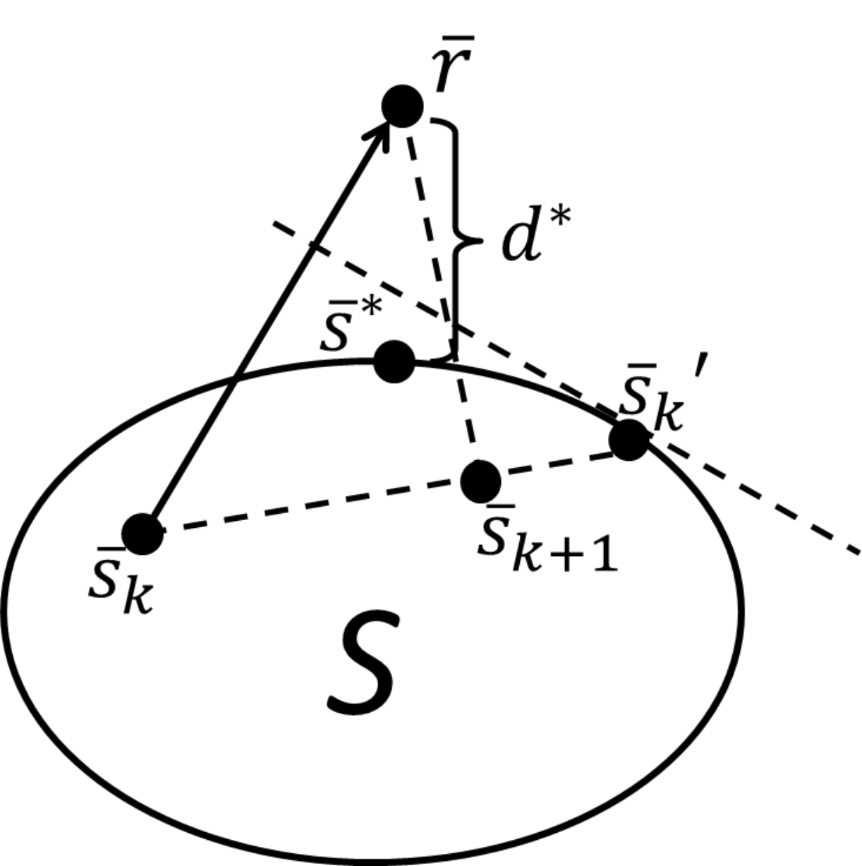
A depiction of a single iteration of Gilbert’s algorithm in 2 dimensions is given in Fig 1
Gilbert’s algorithm with memory
While it can be shown (below) that Gilbert’s algorithm always converges to the optimal distance, sometimes it does so with the lowest possible speed . We have observed that, in some of these instances, the speed of convergence is boosted if we keep a list of the last points returned by the strong optimization oracle, and find the convex combinations of them and that minimizes the distance with respect to . An intuition for why this is a good idea can be seen by considering how the algorithm converges when is a rectangle (see Fig 3) where convergence for Gilbert’s algorithm is but by storing a list , of size 2, convergence is achieved in iterations.
We call the following modification, Gilbert’s algorithm with memory:
- 1.
Choose any .
- 2.
Given , use the oracle to maximize the overlap over all . Add to . If contains entries, erase the first one.
- 3.
Project onto the set . In other words, solve the linear least squares with constraint problem:
subject to (5) where the elements of are arranged as columns in . Set the next point in the algorithm as the solution to Eq. (5), .
- 4.
Go to step 2.
In practice, storing a large number of optimization points makes step 3 time consuming. In fact, the case corresponds to the original weak minimum distance problem. In the implementations discussed in Sections 4 and 5, we balance to trade-off the number of iterations and the time taken for each step.
Gilbert’s algorithm with a heuristic oracle
For some convex sets , the oracle solving OPT is too time consuming. In such cases, a cheaper heuristic algorithm is very advantageous. If the approximate OPT oracle guarantees to return a point, we have the obvious modification of Gilbert’s algorithm, where Step 2 is replaced by
- 2’
Given , use the heuristic to maximize the overlap over all .
If the (decreasing) sequence of distances gets very close to zero, then we have solved WSEP. If, on the contrary, seems to converge to , we can invest time resources and invoke the exact oracle once to maximize the overlap with . Because of the considerations exposed above, if is sufficiently close to the optimal value, then , in which case , as certified by the witness .
We use a heuristic oracle when solving the non-locality of two-qubit Werner states problem in Sec 5.2.
3 Analysis of convergence
In this section we analyze the convergence of Gilbert’s algorithm. We consider the case where we store only a single optimization point, and derive bounds on the convergence for arbitrary sets .
3.1 Polynomial convergence for arbitrary sets
Define the vectors , and and the diameter of the smallest ball containing as
With this notation, the linear inequality at step 2 can be rewritten as , for any , with .
Note that
| (6) |
Then,
| (7) |
for some , with . In Appendix A we show that the value of minimizing the norm of the right hand side of the above equation is given by (4).
There are two possibilities:
- 1.
, or, equivalently, , in which case . Then,
(8) where the last inequality follows from Eq. (6), and the previous one is a consequence of the assumption . We can carry further the approximation and conclude that:
(9) - 2.
, in which case
(10) Substituting this value in eq. (7), it can be verified that , and so
(11) It follows that
(12) Invoking relation (6), we arrive at
(13) Therefore,
(14)
To conclude: no matter what the value of is, we have that
| (15) |
Now, define . Then, the last relation reads:
| (16) |
Since , we have that
| (17) | |||||
where we used (16) to derive the last inequality. The left hand side of relation (17) is a telescopic series; its value is equal to . It follows that , that is:
| (18) |
The algorithm thus converges at least as
| (19) |
In the case , that is , we can improve the latter bound. Indeed, notice that, for we have
| (20) |
this follows from Eqs. (9), (14). Define , with ; we thus have that . Using similar arguments, one concludes that , and, consequently,
| (21) |
If , the scaling of the algorithm to solve WDIST is bounded by
It rests to ascertain how good this method is to solve WSEP. Clearly, if , by eq. (19) we have that calls to the oracle would be enough to find a point with . If, on the contrary, , we would like to find a witness to detect that . In Appendix B, it is shown that this is possible provided that . Invoking bound (21), we thus have that are required. This last bound hence captures the worst-case general performance of the scheme to solve WSEP().
Let us suppose now that actually belongs to the interior of the set , and let be the distance between and the boundary of . That is:
| (22) |
Given , define , and . From the equation above, we have that .
Now, . It follows that , and so, by (12) we have that, for ,
| (23) |
Setting in eq. (8), we have that the case does not occur, unless . In either case, the above expression always holds, and so
| (24) |
Iterating, we find that
| (25) |
The convergence of the algorithm for inner points has an exponential boost.
3.2 Curved sets
We now consider the convergence of Gilbert’s algorithm when the boundary of is curved. Let be an arbitrary point on the boundary of . Then we can always find a tangent half-space of the form , with , such that . can thus be regarded as a rough outer linear approximation to , see Figure 2.
We say that is curved if this approximation can be refined into a quadratic constraint. More specifically, has curvature iff, for any point on the boundary of , with tangent half-space , the set of points
| (26) |
also contains . A set is called strictly convex if and only if .

Now, suppose that has curvature , and consider the point derived from in the second step of Gilbert’s algorithm. Clearly, belongs to the boundary. Moreover, by construction, it has a tangent half-space . From our definition of curvature it hence follows that must belong to the set (26), with . Now, calling , we have that
| (27) |
where the last inequality follows from Eq. (26).
For the case , this last relation, together with Eq. (12), implies that
| (28) |
the last inequality being a consequence of (6). We thus have that
| (29) |
For the case , we have by (9) that
| (30) |
Defining , we hence obtain the recursive relation
| (31) |
with
| (32) |
It is easy to verify that , and therefore
| (33) |
If is comparable to and the curvature is not so small, we should hence expect Gilbert’s algorithm to approach the optimal solution exponentially fast.
For small , however, the number of iterations to solve WDIST is bounded by
| (34) | ||||
| (35) |
In the absence of a promise on the value of , we can estimate the speed of convergence of Gilbert’s algorithm by taking the second inequality of eq. (29) and then approximating by in the right hand side. We thus find that
| (36) |
Similarly as in the previous section, we find that
| (37) |
In other words, the number of iterations to solve WDIST is .
What about WSEP? If , we find, by Appendix B and (35), that a witness will be produced after iterations. If, on the other hand, , by the equation above we find that a point at a distance will be found after calls to the oracle. Hence, in worst-case scenarios, the total number of calls is .
4 How accurate are the bounds?
Let us investigate whether the bounds (18), (21) are asymptotically tight. A possible convex set where the speed of convergence may be computed exactly is the rectangle depicted in Figure 3. Note that in this setting the value of decreases as Gilbert’s algorithm approaches : in view of Eq. (12) it is hence likely that the speed of convergence is low.

Let us first test the accuracy of bound (21). Remember that such a bound only applies when . Identifying the point with the origin of coordinates, take and set the upper vertices of the rectangle to be . Our initial point will be . Figure 4 shows a numerical plot of versus the logarithm of the number of iterations of Gilbert’s algorithm. The plot can be well fitted by an equation of the form . These results are thus in great agreement with the theoretical upper bound (21).

To test bound (18), we will use the same settings as before, with the exception of point , that we will set at , i.e., the point will be laying on the center of the side of the rectangle. The results are shown in Figure 5. The resulting curve fits very well the formula , evidencing that the scaling of bound (18) in worst-case scenarios is correct.

Finally, we test the exponential bound for inner points. Choosing the other two vertices of the rectangle to lie in and , respectively, and taking the inner point , we obtain the plot of Figure 6.

Again, the match between the theory and practice is remarkable.
As we saw in Section 3.2, the above general bounds are not tight when applied to sets with a smooth surface: studying the convergence of the algorithm in less ‘polyhedric’ sets is hence important. An interesting (curved) set where the convergence rate can be easily calculated is a circle.
Setting the origin of coordinates in the center of a circle of radius 1, we placed the external point at , and took to be the initial input for Gilbert’s algorithm. The outputs of Gilbert’s algorithm are plotted in Figure 7, and show an unequivocal exponential convergence.

Figure 3 shows how storing previous optimization points can improve convergence. After only two iterations, Gilbert’s algorithm with a memory buffer of optimization points finds ; contrasting with the polynomial convergence fitted as . Figure 8 shows a further example of this dramatic improvement in the convergence for a set defined as the convex hull of points in dimension . For sufficiently large values of approximately the convergence mimics that of a curved set and after iterations returns as it is contained in .
5 Applications
The original motivation for this paper comes from quantum information theory, where an important primitive consists in deciding whether a vector of experimental data measured by two or more experimentalists is classical, in the sense that it admits a local hidden variable model [4]. The set of all classical vectors forms a convex set whose extreme points correspond to local deterministic strategies. The separation problem for this set is, however, NP-hard when we identify the input size of the problem with the number of measurement settings available to each experimenter [5].
We find that our algorithm allows us to solve instances of WSEP of input size . Our algorithm thus improves on the works of Gondzio et al. [6, 7] and Schwartz et al. [8], where the cases , could not be respectively overcome. Note that the time complexity of the best algorithm known for the strong optimization problem scales as ; for it is therefore impractical to call it more than a few times. Hence, following Section 2, we used a heuristic method to carry out all linear optimisations but the last one. Independently of our work, Montina and Wolf have also used Gilbert’s algorithm together with a heuristic to solve large instances of WSEP in the locality problem [11].
In the next section, we briefly introduce the notions of Bell correlations and EPR steering correlations, where we restrict ourselves to joint terms in the correlations (i.e. neglect local marginals). The first one gives rise to the device-independent framework of quantum correlations (neither parties are trusted) [12], whereas the other one defines a semi-device-independent framework (Alice’s side is untrusted and Bob’s side is trusted) [13]. After the introduction we discuss three applications: In Sec. 5.2, the nonlocality of two-qubit Werner states are investigated, where we improve the known upper bound of the critical visibility and correspondingly beat the known lower bounds on the Grothendieck constant of order 3 (denoted by ). In Sec. 5.3, we study the nonlocality of noisy three-qubit GHZ states, where we provide a Bell inequality which improves the noise tolerance of this state. Finally, in Sec. 5.4, we discuss the EPR-steerability of the two-qubit Werner state using a special configuration of sharp qubit observables. Our obtained critical value for steerability also defines a bound on the joint measurability of the noisy version of these observables.
5.1 Bell and EPR steering correlations
We stick to the so-called correlation scenario (two parties with two measurement outcomes considering only joint correlation terms). A behavior (or a correlator) is a point , where stands for the number of measurement settings per party. Classical behavior is defined by the convex hull of all deterministic behaviors (vertices), which form the so-called correlation polytope . For a given , a vertex labeled by is defined by a specific assignment of , and , , such that the corresponding vertex is given by an matrix with entries . This amounts to distinct vertices (or deterministic strategies). The factor comes from the fact that the inversion , for all defines the same vertex. Any classical behavior is a convex combination with positive weights .
On the other hand, in quantum theory a correlation point may not be expressed as according to Bell’s theorem [4]. In general, the entries of are given by the formula
| (38) |
where is an arbitrary state on (i.e. a trace 1 positive matrix in dimension ) , whereas and are traceless dichotomic observables (i.e. , ) acting on Alice’s and Bob’s system, respectively.
A two-qubit Werner state is as follows [14]
| (39) |
where is the two-qubit singlet . The measurements are traceless qubit observables and , where and are unit vectors in (the so-called Bloch vectors) and denotes the vector of Pauli matrices with components , and . In the above formula (39), is the visibility of the Werner state and the entry of the correlation point is simply given by the dot product
| (40) |
due to Eq. (38). The value of the critical for which becomes a classical behavior no matter the choice of the unit vectors and is unknown for . In particular, the critical value in case of going to infinity, , is known to be equal to . However, its exact value is still unknown. Earlier bounds from the literature imply . Note, however, that Krivine’s upper bound [15, 16] has been recently improved to the value [17]. In this paper, we improve on the lower bound value [18, 19] establishing a new lower bound value of .
It is straightforward to extend the two-party correlation scenario discussed above to three parties, in which case we pick the noisy Greenberger-Horne-Zeilinger state [20]
| (41) |
where . For a fixed number of settings per party, the quantum behavior is given by its entries
| (42) |
where , , are traceless dichotomic qubit observables. Besides, the deterministic behaviors of the three-party correlation polytope for a given are given by the vertices with entries , where , , may take all possible combinations of values, which amounts to vertices. Similarly to the case of bipartite Werner states, we ask for a given the critical value of , denoted by , above which the point cannot be expressed as a convex combination of deterministic strategies . We are particularly interested in the case of , which we denote by . In case of , the critical value is known to be [20], which gives an upper bound to . The best upper bound for so far is attained in Ref. [21] in case of settings per party: . In this paper, we decrease this upper bound down to (using 16 measurements per party).
Lastly, we present an application in the EPR steering scenario [22] (and see [13] for a recent review of the field). Here we consider again the case of two-qubit Werner states. However, instead of the fully device-independent Bell scenario, this time we assume a semi-device independent scenario, where only Alice’s system is uncharacterized whereas Bob’s measurements are assumed to be well defined. In particular, we can assume without loss of generality that Bob performs three Pauli measurements , and . Plugging these special measurement directions into (40), we get the quantum behavior with entries
| (43) |
where . On the other hand, in the steering scenario (unlike the Bell scenario) the region of classical correlations is defined by a (still convex) set with a continuous number of extremal points. This region is characterized by the convex hull of the following points:
| (44) |
where the pure qubit states and for and . Note that in this scenario the value is known to be [13], although in principle it can only be achieved exactly in the limit of infinitely many measurement settings. Here we find via a steering inequality in case of Alice performing measurements in the buckyball configuration. There is a link between EPR steering and jointly measurability [23]. In combination with our result, the set of noisy version of the sharp measurements , in the buckyball configuration are incompatible for and leads to steering when applied to an arbitrary entangled pure state. To the best of our knowledge, the largest set of measurements investigated in the literature corresponds to the dodecahedron, which has 20 vertices and these directions determine settings leading to the visibility [24]. Hence, our bound considerably improves on this value as well.
5.2 Nonlocality of two-qubit Werner states
Due to Tsirelson [25], . In that case, the correlation polytope is well characterized and the only nontrivial facet corresponds to the CHSH-Bell inequality [26], whose maximal violation implies the above value . Up to , the correlation polytope is completely resolved and two new facets are obtained beyond the CHSH one [27]. None of them decreases the critical visibility, hence . For higher the complexity of the polytope grows rapidly, hence a complete characterization becomes challenging even for moderate . For instance, in case of Avis et al. [27] gives a lower bound of to the number of inequivalent facets. Nevertheless, it is known that [18]. Using the algorithm described in Sec. 2, we prove that even , hence 24 measurement settings are enough to overcome the limit corresponding to the CHSH inequality. The question of the smallest number of measurements such that is still open, however, we conjecture that either is the correct number or it is very close to it. The algorithm in Sec. 2 also allows us to show that which in turn shows that (beating the best bound currently known). In addition, an example is presented where the measurement vectors , feature a nice configuration on the Bloch sphere, associated with the truncated icosahedron (the so-called buckyball configuration), showing that .
Below we present how the algorithm in Sec. 2 is applied to our problem. Given a fixed measurement configuration with Bloch vectors , , , the method is as follows. We pick a value of which we wish to beat, say, . The above Bloch vectors along with define a quantum point with entries according to Eq. (40), which we conjecture to lie (slightly) outside the correlation polytope . Given and the polytope we call the algorithm to solve the weak separation problem WSEP, i.e., it outputs a separating hyperplane with norm , such that
| (45) |
where denotes transposition of the matrix . This certifies that is indeed outside the polytope and implies the upper bound
| (46) |
As discussed in Sec. 2, within each iteration the algorithm uses an approximate Oracle (the description of such a procedure can be found in Appendix A of Ref. [17]), and it is enough to use an exact Oracle in the very last iteration which computes the value of correctly via a brute force search. Note that in the exact evaluation of the left-hand side of Eq. (45), it suffices to compute the maximum over all deterministic strategies of Bob (which can be further divided by 2 due to the absolute sign):
| (47) |
In Matlab, fast matrix manipulation allows us to evaluate parallel the right-hand side expression in several variables. Furthermore, the usage of an Nvidia 4GB graphics card in our standard desktop PC could still boost the speed with roughly a factor of 3. Eventually, this allowed us to compute the value for settings in (47) within one week.
The above described method is optimal for a fixed configuration, however, it is expected to arrive at better upper bounds on by varying the measurement directions and as well. In the original formulation of the algorithm in Sec. 2 this was not possible, however, we can call the algorithm in an iterative manner such that it can search for optimized measurements as well. It works as follows:
- 1.
Fix . Generate initial Bloch vectors and , (either randomly or corresponding to some nice geometric configuration). Also, set .
- 2.
Construct point with coordinates .
- 3.
Given polytope and point , run the algorithm in Sec. 2 to get a hyperplane with norm and a value of the witness.
- 4.
Maximize the Bell witness within the two-qubit quantum set, thus obtaining a point . This can be done either with a heuristic search or using an SDP [28] implementing the zeroth level of the NPA hierarchy [29]. In the latter case, however, we also have to ensure that the is realizable with two qubits.
- 5.
Decrease slightly and construct the point .
- 6.
Go to step 3 until .
Both for and , we run the iterative procedure above optimizing the measurements as well. Whereas in case of , we chose the 60-vertex truncated icosahedron as the fixed measurement configuration both for Alice and Bob (note that the vertices of this geometry possess an inversion symmetry, and it is enough to choose only half of the vertices). In all the above cases, we run the algorithm in step 3 without memory buffer, which makes this step very fast (although, the number of iterations may become bigger). In a supplementary Mathematica file added to the arXiv submission, we give detailed results of the final measurement directions, the Bell matrices and the corresponding local bound . In case of , ten million iterations were used in Gilbert’s algorithm of Sec. 2 by setting . In cases of and , we decreased from down to with step size in the above described iterative manner, running the algorithm in step 3 ten thousand times. The following upper bounds on the critical visibility of the Werner states were obtained: , , and . To the best of our knowledge, this last value provides the best lower bound to .
5.3 Nonlocality of noisy GHZ states
We use Gilbert’s algorithm to improve on the smallest upper bound of 0.4960 on in case of the noisy three-qubit GHZ state (41). To this end, let us arrange the qubit observables , , in the plane as follows
| (48) |
For a fixed number of settings per party, the quantum point is given by its entries
| (49) |
Let us in particular choose and for , resulting in
| (50) |
where .
Similarly to Sec. 5.2, we run Gilbert’s algorithm in Sec. 2 with the above setting (i.e., the value we wish to beat) using 10 million iterations. The results along with the Bell witness and the local bound are summarized in a supplementary Mathematica file. Plugging these values into the respective formula (46):
we get the upper bound , which defines an upper bound to the critical value too.
Let us mention, however, that the use of modified Gilbert’s algorithm is not restricted to Bell scenarios with correlation polytopes. It can be used in any Bell scenario (more than two parties with more than two outputs including marginal terms as well). Moreover, we expect Gilbert’s algorithm to be useful in other tasks as well, such as quantum communication complexity [30] or dimension witnesses [31] (given an efficient characterization of dimension restricted quantum correlations [32]). Another potential application is the case of EPR steering for which we show benchmark results in the next subsection.
5.4 EPR steering of two-qubit Werner states
We use the modified Gilbert’s algorithm with memory buffer in Sec. 2 and find an upper bound of on the steerability limit of the two-qubit Werner state for Alice’s measurements carried out in the buckyball configuration. In particular, we fix and generate the quantum point in Eq. (43) using the buckyball configuration for Alice’s unit vectors , . Given this point and the description of the convex unsteerable set (44), we run the modified Gilbert’s algorithm with memory buffer to find the witness which separates from this set. In case of , the Oracle to be solved
| (51) |
where denotes the largest eigenvalue of a matrix , is too costly, hence similarly to Secs. 5.2 and 5.3 we use an approximate Oracle to compute the maximum in Eq. (51). This is done via a see-saw type iterative search as follows:
- 1.
Choose random assignments , for Alice’s deterministic strategy.
- 2.
Construct the matrix .
- 3.
Compute the eigenvector corresponding to the larger eigenvalue of .
- 4.
Set if , otherwise set for all .
- 5.
Go back to step 2 until convergence of is reached.
In the particular implementation, we run the above method 100 times and pick the largest final , which gives an even more reliable approximation of in formula (51).
Table 1 shows the performance of the Gilbert algorithm of Sec. 2 using different memory sizes and number of iterations in terms of distances of from the unsteerable set of points. In complete agreement with the findings of Sec. 4, the use of memory speeds up convergence considerably. For instance, in case of , convergence of is already attained up to 7th digit for iterations. However, without memory (i.e. the case of ), even is far from reaching convergence. The steering witness matrix (after rescaling and truncation) corresponding to (, ) is given in a supplementary Mathematica file, which also provides the unsteerable value defined by Eq. (51) and the maximal quantum value
of the witness. According to Eq. (46), we then get the upper bound
on the steerability limit of the two-qubit Werner state for the buckyball measurement configuration.
References
- [1] M. Grötschel, L. Lovasz and A. Schrijver, Geometric Algorithms and Combinatorial Optimization, Springer 1985.
- [2] H. Crowder and M. W. Padberg, Solving large-scale symmetric travelling salesman problems to optimality, Management Science 26, 495-509 (1980).
- [3] W. H. Cunningham (1984), Testing membership in matroid polyhedra, Journal of Combinatorial Theory (B) 36 161-188 (1984).
- [4] J. S. Bell, On the Einstein-Poldolsky-Rosen paradox, Physics 1, 195–200 (1964).
- [5] I. Pitowsky, Quantum Probability, Quantum Logic, Lecture Notes in Physics 321, Heidelberg, and Springer, 1989.
- [6] J. Gondzio, Interior point methods 25 years later, European Journal of Operational Research 218, 587–601 (2012).
- [7] J. Gondzio, J. Gruca, J. Hall, W. Laskowski, M. Żukowski, Solving Large-Scale Optimization Problems Related to Bell’s Theorem, arXiv:1204.3587 (2012).
- [8] S. Schwarz, A. Stefanov, S. Wolf, A. Montina, Phys. Rev. A 94, 022322 (2016).
- [9] Lawrence M. Ioannou, Benjamin C. Travaglione, and Donny Cheung, Convex Separation from Optimization via Heuristics, arXiv:cs/0603089 (2006).
- [10] E. G. Gilbert, An iterative procedure for computing the minimum of a quadratic form on a convex set, SIAM J. Contrl., vol. 4, pp. 61-80, 1966.
- [11] A. Montina and S. Wolf, Can non-local correlations be discriminated in polynomial time?, arXiv:1609.06269 (2016).
- [12] N. Brunner, D. Cavalcanti, S. Pironio, V. Scarani, and S. Wehner, Bell nonlocality, Rev. Mod. Phys. 86, 419–478 (2014); V. Scarani, arXiv:1303.3081 (2013).
- [13] D. Cavalcanti and P. Skrzypczyk, Quantum steering: a short review with focus on semidefinite programming, arXiv:1604.00501 (2016).
- [14] R. F. Werner, Quantum states with Einstein-Podolsky-Rosen correlations admitting a hidden-variable model, Phys. Rev. A 40, 4277–4281 (1989).
- [15] J. L. Krivine, Adv. Math. 31, 16 (1979).
- [16] A. Acín, N. Gisin, and B. Toner, Grothendieck’s constant and local models for noisy entangled quantum states, Phys. Rev. A 73, 062105 (2006).
- [17] F. Hirsch, M. T. Quintino, T. Vértesi, M. Navascués, and N. Brunner, Better local hidden variable models for Werner states and an upper bound on the Grothendieck constant , in preparation.
- [18] T. Vértesi, More efficient Bell inequalities for Werner states, Phys. Rev. A 78, 032112 (2008).
- [19] B. Hua, M. Li, T. Zhang, C. Zhou, X. Li-Jost, S.-M. Fei, Towards Grothendieck Constants and LHV Models in Quantum Mechanics, J. Phys. A: Math. Theor. 48, 065302 (2015).
- [20] D.M. Greenberger, M.A. Horne, and A. Zeilinger, Bells Theorem, Quantum Theory, and Conceptions of the Universe (ed. M. Kafatos, Kluwer Academic, Dordrecht, Holland, 1989), p. 69.
- [21] T. Vértesi and K.F. Pál, Phys. Rev. A 84, 042122 (2011).
- [22] H.M. Wiseman, S.J. Jones and A.C. Doherty, Phys. Rev. Lett. 98, 140402 (2007); S. J. Jones, H.M. Wiseman and A.C. Doherty, Phys. Rev. A 76, 052116 (2007).
- [23] M. T. Quintino, T. Vértesi, and N. Brunner, Phys. Rev. Lett. 113, 160402 (2014); R. Uola, T. Moroder, and O. Gühne, Phys. Rev. Lett. 113, 160403 (2014).
- [24] D. J. Saunders, S. J. Jones, H. M. Wiseman and G. J. Pryde, Experimental EPR-Steering using Bell-local States, Nat. Phys. 6, 845-849 (2010); R. Uola, K. Luoma, T. Moroder, and T. Heinosaari, Adaptive strategy for joint measurements, arXiv:1604.08724 (2016).
- [25] B. S. Tsirelson, J. Soviet Math. 36, 557 (1987).
- [26] J.F. Clauser, M.A. Horne, A. Shimony, R.A. Holt, Phys. Rev. Lett. 23, 880 (1969).
- [27] D. Avis, H. Imai and T. Ito, J. Phys. A 39, 11283–11299 (2006).
- [28] S. Boyd and L. Vandenberghe, Convex optimization, Cambridge University Press (2004).
- [29] M. Navascues, S. Pironio, A. Acin, Phys. Rev. Lett. 98, 010401 (2007).
- [30] H. Buhrman, R. Cleve, S. Massar, and R. de Wolf, Nonlocality and communication complexity, Rev. Mod. Phys. 82, 665 (2010).
- [31] N. Brunner, S. Pironio, A. Acin, N. Gisin, A. A. Methot, and V. Scarani, Testing the dimension of hilbert spaces, Phys. Rev. Lett. 100, 210503 (2008).
- [32] M. Navascues, A. Feix, M. Araujo, and T. Vertesi, Characterizing finite-dimensional quantum behavior, Phys. Rev. A 92, 042117 (2015).
Appendix A: computation of
The purpose of this Appendix is to prove that the value of that makes the norm of the right-hand side of eq. (7) minimal is given by eq. (4).
First, note that can be decomposed as
| (52) |
where . By varying the value of , we must minimize the coefficient . Now, , with equality iff . Indeed, suppose that , then we have that
| (53) |
which only makes sense if .
It follows that, unless , the value of minimizing the norm of the right hand side of eq. (52) will be greater than . Clearly, if , then the optimal value is , in which case . Otherwise, for all values of , the coefficient will be non-positive, and hence the value of minimizing the aforementioned coefficient -and so the norm of the right hand side of eq. (52)- is .
Appendix B: Stopping criterion for the Separation problem
Every call to OPT in step 2 of Gilbert’s algorithm returns a vector such that
| (54) |
for all . Consequently, any iteration such that can be interpreted as a proof that . Indeed, if , then , hence contradicting the above equation.
When should we expect this to happen? Let . By Eq. (1), we have that .
Now,
| (55) |
A sufficient condition for the stopping criterion to hold is thus that the right hand side of the above equation is positive, which can be shown equivalent to:
| (56) |