Ensemble-Based Algorithms to Detect Disjoint and Overlapping Communities in Networks
Abstract
Given a set of community detection algorithms and a graph as inputs, we propose two ensemble methods EnDisCo and MeDOC that (respectively) identify disjoint and overlapping communities in . EnDisCo transforms a graph into a latent feature space by leveraging multiple base solutions and discovers disjoint community structure. MeDOC groups similar base communities into a meta-community and detects both disjoint and overlapping community structures. Experiments are conducted at different scales on both synthetically generated networks as well as on several real-world networks for which the underlying ground-truth community structure is available. Our extensive experiments show that both algorithms outperform state-of-the-art non-ensemble algorithms by a significant margin. Moreover, we compare EnDisCo and MeDOC with a recent ensemble method for disjoint community detection and show that our approaches achieve superior performance. To the best of our knowledge, MeDOC is the first ensemble approach for overlapping community detection.
I Introduction
Community detection (CD) has found applications in social, biological, business, and other kinds of networks. However, CD algorithms suffer from various flaws – (i) Most existing CD algorithms are heavily dependent on vertex ordering [11], yielding completely different community structures when the same network is processed in a different order. For example, Figure 1(a) shows dissimilar community structures after running InfoMap [30] on different vertex orderings of the Football network [7]. (ii) Most optimization algorithms may produce multiple community structures with the same “optimal” value of the objective function. For instance, in Figure 1(b), assigning vertex to either or results in the same modularity score [24]. (iii) Different CD algorithms detect communities in different ways, e.g., as dense groups internally [25], or groups with sparse connections externally [10]. It is therefore natural to think of an ensemble approach in which the strengths of different CD algorithms may help overcome the weaknesses of any specific CD algorithm. Some preliminary attempts have been made by [8, 20]11 1 Note that ensemble approaches have proved successful in clustering and classification [33]..

Contributions. In this paper, we design two ensemble CD algorithms. The EnDisCo algorithm runs multiple “base” CD algorithms using a variety of vertex orderings to derive a first set of communities. We then consider the memberships of vertices obtained from base CD algorithms as features and derive a latent network using pair-wise similarity of vertices. The final disjoint community structure is obtained by running any CD algorithm again on the latent network. The MeDOC algorithm leverages the fact that many communities returned by base algorithms are redundant and can therefore be grouped into “meta-communities” to avoid unnecessary computation. We use meta-communities to build an association matrix, where each entry indicates the probability of a vertex belonging to a meta-community. Finally, we obtain both disjoint and overlapping community structures via post-processing on the association matrix. To the best of our knowledge, we are the first to propose (i) an ensemble framework for overlapping community detection, and (ii) an overlapping CD algorithm that leverages disjoint community information. We run experiments to identify the best parameter settings for EnDisCo and MeDOC. Experiments on both synthetic and real-world networks show that our algorithms outperform both the state-of-the-art non-ensemble based methods [2, 30, 34] and a recently proposed ensemble approach [20] by a significant margin22 2 We report -values for all our experiments to show statistical significance.. We also show that our ensemble approaches reduce the effect of vertex ordering.
Note: We use the term “community structure” to indicate the result (set of “communities”) returned by an algorithm. Each community is a set of vertices.
II Related Work
There has been a great deal of work on clustering data using ensemble approaches (see [33] for a review). However, when it comes to clustering vertices in networks, ensemble approaches have been relatively scarce33 3 See the survey [10] for various community detection algorithms.. Dahlin and Svenson [8] were the first to propose an instance-based ensemble CD algorithm for networks which fuses different community structures into a final representation. A few methods addressed the utility of merging several community structures [29]. A new ensemble scheme called CGGC was proposed to maximize modularity [26]. Kanawati proposed YASCA, an ensemble approach to different network partitions derived from ego-centered communities computed for each selected seed [16]. He further emphasized the quality and diversity of outputs obtained from the base algorithms for ensemble selection [17].
A “consensus clustering” [20] approach was recently proposed which leverages a consensus matrix to produce a disjoint community structure which outperformed previous approaches. Our work differs from this approach in at least three significant ways: (i) they measure the number of times two vertices are assigned to the same community, thus ignoring the global similarity of vertices; whereas we capture the global similarity by representing the network within a feature space and grouping redundant base communities into meta communities; (ii) they either take multiple algorithms or run a particular algorithm multiple times for generating an ensemble matrix, whereas we consider both options; (iii) we are the first to show how aggregating multiple disjoint base communities can lead to discover both disjoint and overlapping community structures simultaneously. We show experimentally that EnDisCo beats consensus clustering.
III EnDisCo: Ensemble-based Disjoint Community Detection
EnDisCo (Ensemble-based Disjoint Community Detection) starts by first using different CD algorithms to identify different community structures. Second, an “involvement” function is used to measure the extent to which a vertex is involved with a given community, which in turn sets the posterior probabilities of each vertex belonging to different communities. Third, EnDisCo transforms the network into a feature space. Fourth, an ensemble matrix is constructed by measuring the pair-wise similarity of vertices. Finally, we apply any standard CD algorithm on the ensemble matrix and discover the final disjoint community structure.
III-A Algorithmic Description
EnDisCo follows three fundamental steps (a pseudo-code is shown in Algorithm 1):
(i) Generating base partitions. Given a network and a set of different base CD algorithms, EnDisCo runs each algorithm on different vertex orderings (randomly selected) of . This generates a set of different community structures denoted , where each community structure constitutes a specific partitioning of vertices in , and each might be of different size (Step 1).
(ii) Constructing ensemble matrix. Given a , we then compute the extent of ’s involvement in each community in via an “involvement” function (Step 1). Possible definitions of are given in Section III-B. For each vertex , we construct a feature vector whose elements indicate the distance of (measured by ) from each community obtained from different runs of the base algorithms (Step 1). The size of is same as the number of communities in (approx. , where is the average size of a base community structure). Let be the largest distance of from any community in the sets in (i.e., in Step 1). We define the conditional probability of belonging to community (Step 1) as:
| (1) |
The numerator ensures that the greater the distance of from community , the less likely is to be in community . The normalization factor in the denominator ensures that . Add-one smoothing in the numerator allows a non-zero probability to be assigned to all s, especially for such that .
The set of posterior probabilities of is: (Step 1), which in turn transforms a vertex into a point in a multi-dimensional feature space. Finally we construct an ensemble matrix whose entry is the similarity (obtained from a function whose possible definitions are given in Section III-B) between the feature vectors of and (Step 1). The ensemble matrix ensures that the more communities a pair of vertices share the more likely they are connected in the network [34].
III-B Parameter Selection
Involvement Function (): We use two functions to measure the involvement of a vertex in a community : (i) Restricted Closeness Centrality (): This is the inverse of the average shortest-path distance from the vertex to the vertices in community , i.e., ; (ii) Inverse Distance from Centroid (IDC): we first identify the vertex with highest closeness centrality (w.r.t. the induced subgraph of ) in community , mark it as the centroid of (denoted by ), and then measure the involvement of as the inverse of the shortest-path distance between and , i.e., .
Similarity Function (): We consider cosine similarity () and Chebyshev distance () (essentially, ) to measure the similarity between two vectors.
Algorithm for Re-clustering (): we consider each base CD algorithm as the one to re-cluster the vertices from the ensemble matrix. The idea is to show that a non-ensemble CD algorithm can perform even better when considering the ensemble matrix of network than the adjacency matrix of . However, one can use any CD algorithm in this step to detect the community structure. We will show the effect of different algorithms used in this step in Section V-D2.
Number of Iterations (): Instead of fixing a hard value, we set to be dependent on the number of vertices in the network. We vary from to (with step ) of and confirm that for most of the networks, the accuracy of the algorithm converges at (Figures 2(c) and 2(f)), and therefore we set in our experiments.
III-C Complexity Analysis
Suppose is the number of vertices in the network, is the number of base algorithms and is the number of vertex orderings. Further suppose is the average size of the community structure. Then the loop in Step 1 of Algorithm 1 would iterate times (where ). The construction of the ensemble matrix in Step 1 would take . Graph partitioning is NP-hard even to find a solution with guaranteed approximation bounds — however, heuristics such as the famous Kernighan-Lin algorithm take time.
IV MeDOC: Meta-clustering Approach
MeDOC (Meta Clustering based Disjoint and Overlapping Community Detection) starts by executing all base CD algorithms, each with different vertex orderings, to generate a set of community structures. It then creates a multipartite network. After this, a CD algorithm is used to partition the multipartite network. Finally, a vertex-to-community association function is used to determine the membership of a vertex in a community. Unlike EnDisCo, MeDOC yields both disjoint and overlapping community structures from the network.
IV-A Algorithmic Description
MeDOC has the following four basic steps (pseudo-code is in Algorithm 2):
(i) Constructing multipartite network. MeDOC takes CD algorithms and runs each on different vertex orderings of . For each ordering , produces a community structure of varying size (Step 2). After running on vertex orderings, each algorithm produces different community structures . Therefore at the end of Step 2, we obtain community structures each from algorithms (essentially, we have community structures). We now construct a -partite network (aka meta-network) as follows: the vertices are members of , i.e., a community present in a community structure obtained from any of the base algorithms in and any vertex ordering, is a vertex of . We draw an edge from a community to a community and associate a weight (Step 2). Possible definitions of will be given later in Section IV-B. Since each is disjoint, the vertices in each partition are never connected.
(ii) Re-clustering the multipartite network. Here we run any standard CD algorithm on the multipartite network and obtain a community structure containing (say) communities . Note that in this step, we indeed cluster the communities obtained earlier in Step 2; therefore each such community obtained here is called a “meta-community” (or community of communities) (Step 2).
(iii) Constructing an association matrix. We determine the association between a vertex and a meta-community by using a function and construct an association matrix of size , where each entry (Step 2). Possible definitions of will be given later in Section IV-B.
(iv) Discovering final community structure. Final vertex-to-community assignment is performed by processing . The entries in each row of denote membership probabilities of the corresponding vertex in communities. For disjoint community assignment, we label each vertex by the community in which possesses the most probable membership in , i.e., . Tie-breaking is handled by assigning the vertex to the community to which most of its direct neighbors belong. Note that every meta-community can not be guaranteed to contain at least one vertex, that in turn can not assure communities in the final community structure. For discovering overlapping community structure, we assign a vertex to those communities for which the membership probability exceeds a threshold . Possible ways to specify threshold will be specified later in Section IV-B.
IV-B Parameter Selection
Matching Function (): Given two communities and , we measure their matching/similarity via Jaccard Coefficient (JC)= and average precision (AP) =.
Association Function (): Given a meta-community consisting of (say,) communities, the association of with can be calculated as , where returns if is a part of , otherwise. For example, if , then . Alternatively, a weighted association measure may assign a score to w.r.t. based on the co-occurrence of the other community members with , i.e., . In our earlier example, .
Threshold (): We choose the threshold automatically as follows. We first assign each vertex to its most probable community – this produces a disjoint community structure. Each vertex is represented by a feature vector which is the entire ’th row of the association matrix . We then measure the average similarity of vertices in as follows: , where is the set of edges completely internal to , is an edge , and is cosine similarity. The probability that two vertices are connected in is then defined as:
| (2) |
For a vertex , if , we further assign to , in addition to its current community. We compare our threshold selection method with the following method: each vertex is assigned to its top high probable communities (we set to or ). Our experiments show that MeDOC delivers excellent performance with our threshold selection method (see Figures 3(g)-(i)).
Other input parameters and remain same as discussed in Section III-B.
IV-C Complexity Analysis
The most expensive step of MeDOC is to construct the multipartite network in Step 3. If is the number of base algorithms, is the number of vertex orderings and is the average size of a base community structure, the worst case scenario occurs when each vertex in one partition is connected to each vertex in other partitions — if this happens, the total number of edges is . However, in practice the network is extremely sparse and leads to edges (because in sparse graphs ). Further, constructing the association matrix would take iterations (where ).
| (a) Networks with disjoint communities | ||||||||||
| Networks | Vertex type | Edge type | Community type | N | E | C | S | Reference | ||
| University | Faculty | Friendship | School | 81 | 817 | 3 | 0.54 | 27 | 1 | [23] |
| Football | Team | Games | Group-division | 115 | 613 | 12 | 0.64 | 9.66 | 1 | [7] |
| Railway | Stations | Connections | Province | 301 | 1,224 | 21 | 0.24 | 13.26 | 1 | [6] |
| Coauthorship | Researcher | Collaborations | Research area | 103,677 | 352,183 | 24 | 0.14 | 3762.58 | 1 | [4, 5] |
| (b) Networks with overlapping communities | ||||||||||
| Networks | Vertex type | Edge type | Community type | N | E | C | S | Reference | ||
| Senate | Senate | Similar voting pattern | Congress | 1,884 | 16,662 | 110 | 0.45 | 81.59 | 4.76 | [15] |
| Flickr | User | Friendship | Joined group | 80,513 | 5,899,882 | 171 | 0.046 | 470.83 | 18.96 | [31] |
| Coauthorship | Researcher | Collaborations | Publication venues | 391,526 | 873,775 | 8,493 | 0.231 | 393.18 | 10.45 | [27] |
| LiveJournal | User | Friendship | User-defined group | 3,997,962 | 34,681,189 | 310,092 | 0.536 | 40.02 | 3.09 | [34] |
| Orkut | User | Friendship | User-defined group | 3,072,441 | 117,185,083 | 6,288,363 | 0.245 | 34.86 | 95.93 | [34] |
V Results of Disjoint Community Detection
V-A Datasets
We use the LFR benchmark model [19] to generate synthetic networks with ground-truth community structure by varying the number of vertices , mixing parameter (the ratio of inter- and intra-community edges), average degree , maximum degree , minimum (maximum) community size (), average percentage of overlapping vertices and the average number of communities to which a vertex belongs.44 4 Unless otherwise stated, we generate networks with the same parameter configuration used in [6, 16, 3]: , , , , , , , . Note that for each parameter configuration, we generate 50 LFR networks, and the values in all the experiments are reported by averaging the results. We also use real-world networks mentioned in Table I(a) for experiments (see detailed description in Appendix [1]).
V-B Baseline Algorithms
We compare EnDisCo and MeDOC with the following algorithms: (i) Modularity-based: FastGreedy (FstGrdy) [25], Louvain (Louvain) [2] and CNM [7]; (ii) Vertex similarity-based: WalkTrap (WalkTrap) [28]; (iii) Compression-based: InfoMap (InfoMap) [30]; (iv) Diffusion-based: Label Propagation (LabelPr) [29]. These algorithms are also used as base algorithms in in our ensemble approaches. We further compare our methods with Consensus Clustering (ConsCl) [20], a recently-proposed ensemble-based framework for disjoint community detection.
V-C Evaluation Metrics
As we know the ground-truth community structure, we measure performance of competing CD algorithms using the standard Normalized Mutual Information (NMI) [9] and Adjusted Rand Index (ARI) [14].

| Algorithm | Synthetic Networks | Real-world Networks | Average over | |||||||||||||||||||||
| LFR () | LFR () | LFR () | Football | Railway | University | Coauthorship | All Networks | |||||||||||||||||
| E | M | E | M | E | M | E | M | E | M | E | M | E | M | E | M | C | ||||||||
| FstGrdy | 2.39 | 2.93 | 2.71 | 3.02 | 3.81 | 3.92 | 0 | 0 | 1.22 | 1.43 | 2.20 | 2.86 | 3.98 | 4.60 | 2.33 | 2.36 | 1.98 | |||||||
| Louvain | 1.97 | 2.04 | 2.22 | 2.40 | 3.41 | 3.86 | 0 | 0 | 1.17 | 1.43 | 2.12 | 2.30 | 2.21 | 2.39 | 1.99 | 2.01 | 1.98 | |||||||
| CNM | 2.07 | 2.46 | 2.14 | 2.83 | 3.22 | 3.50 | 1.23 | 1.46 | 1.49 | 1.92 | 2.39 | 2.40 | 2.92 | 3.41 | 2.20 | 2.42 | 2.01 | |||||||
| InfoMap | 0 | 0 | 1.44 | 1.62 | 2.01 | 2.46 | 0 | 0 | 1.22 | 1.56 | 2.01 | 2.20 | 2.31 | 2.98 | 1.28 | 1.31 | 1.28 | |||||||
| WalkTrap | 4.43 | 4.97 | 4.86 | 5.08 | 6.98 | 7.42 | 2.21 | 2.46 | 3.21 | 3.49 | 4.22 | 4.49 | 5.06 | 5.51 | 4.24 | 4.65 | 4.01 | |||||||
| LabelPr | 5.06 | 5.72 | 5.12 | 5.39 | 7.50 | 7.82 | 3.01 | 3.29 | 3.46 | 3.79 | 6.21 | 6.80 | 6.21 | 6.98 | 5.21 | 5.46 | 3.76 | |||||||
| (A) | (B) | |||||||||||||||||||||||
V-D Experimental Results
We first run experiments to identify the best parameters for EnDisCo and MeDOC and then present the comparative analysis among the competing algorithms.
V-D1 Dependency on the Parameters
We consider the LFR networks and vary . Figure 2(a) shows that the accuracy of EnDisCo is similar for both the involvement functions, while Figure 2(b) shows cosine similarity fully dominating Chebyshev distance. Figure 2(d) shows that Jaccard coefficient performs significantly better than average precision when MeDOC is considered, while Figure 2(e) shows that the weighted association function seems to dominate the other for and exhibits similar performance for . We further vary the number of iterations to obtain communities with different vertex orderings – Figures 2(c) and 2(f) show that for the networks with strong community structure (such as LFR (), Football), the accuracy levels off at ; however with increasing leveling off occurs at larger values of . Note that the patterns observed here for LFR network are similar for other networks. Therefore unless otherwise stated, in the rest of the experiment we show the results of our algorithms with the following parameter settings for disjoint community detection: EnDisCo: , , ; MeDOC: , , .
V-D2 Impact of Base CD Algorithms on EnDisCo and MeDOC
In order to assess the impact of each base algorithm in our ensemble, we measure the accuracy of EnDisCo and MeDOC when that base algorithm is removed from the ensemble — Table III shows that for LFR networks InfoMap has the biggest impact on accuracy according to both the evaluation measures (NMI and ARI) for both EnDisCo and MeDOC (results are same for real networks [1]).
As the final step in both EnDisCo and MeDOC is to run a CD algorithm for re-clustering, we also conduct experiments (Table IV for LFR networks and Appendix [1] for real networks) to identify the best one. Again, InfoMap proves to be the best.
| No. | Base | Disjoint | Overlapping | ||||
|---|---|---|---|---|---|---|---|
| Algorithm | EnDisCo | MeDOC | MeDOC | ||||
| NMI | ARI | NMI | ARI | ONMI | |||
| (1) | All | 0.85 | 0.89 | 0.87 | 0.90 | 0.84 | 0.87 |
| (2) | (1) FstGrdy | 0.83 | 0.88 | 0.84 | 0.88 | 0.83 | 0.85 |
| (3) | (1) Louvain | 0.82 | 0.86 | 0.85 | 0.86 | 0.81 | 0.84 |
| (4) | (1) CNM | 0.82 | 0.85 | 0.83 | 0.87 | 0.82 | 0.85 |
| (5) | (1) InfoMap | 0.80 | 0.81 | 0.81 | 0.82 | 0.80 | 0.81 |
| (6) | (1) WalkTrap | 0.84 | 0.88 | 0.85 | 0.81 | 0.83 | 0.86 |
| (7) | (1) LabelPr | 0.84 | 0.87 | 0.86 | 0.87 | 0.83 | 0.85 |
| Re-clustering | Disjoint | Overlapping | ||||
|---|---|---|---|---|---|---|
| Algorithm | EnDisCo | MeDOC | MeDOC | |||
| NMI | ARI | NMI | ARI | ONMI | ||
| FstGrdy | 0.79 | 0.80 | 0.80 | 0.83 | 0.81 | 0.84 |
| Louvain | 0.82 | 0.84 | 0.83 | 0.86 | 0.82 | 0.83 |
| CNM | 0.83 | 0.81 | 0.83 | 0.86 | 0.81 | 0.80 |
| InfoMap | 0.85 | 0.89 | 0.87 | 0.90 | 0.84 | 0.87 |
| WalkTrap | 0.75 | 0.78 | 0.77 | 0.82 | 0.76 | 0.79 |
| LabelPr | 0.77 | 0.79 | 0.78 | 0.80 | 0.75 | 0.77 |
V-D3 Comparative Evaluation
Table II(A) reports the performance of our approaches on all networks using different algorithms in the final step of EnDisCo and MeDOC. The numbers denote relative performance improvement of our algorithms (E:EnDisCo M:MeDOC) w.r.t. a given algorithm when that algorithm is used in the final step. For instance, the first entry in the last row (5.06) means that for LFR () network, the accuracy of EnDisCo (when LabelPr is used for re-clustering in its final step) averaged over NMI and ARI (0.83) is 5.06% higher than that of LabelPr (0.79). The actual values are reported in Appendix [1]. The point to take away from this table is that irrespective of which classical CD algorithm we compare against, EnDisCo and MeDOC always improve the quality of communities found. Moreover, we observe from the results of LFR networks that with the deterioration of the community structure (increase of ), the improvement increases for all the re-clustering algorithms. Further, Table II(B) shows the average improvement of EnDisCo and MeDOC when compared against Consensus Clustering (ConsCl). We see that for disjoint networks, both EnDisCo and MeDOC beat ConsCl with MeDOC emerging in top place.
VI Results of Overlapping Community Detection
VI-A Datasets
We again use the LFR benchmark to generate synthetic networks with overlapping community structure with the following default parameter settings as mentioned in [18, 12]: , , , , , , , . We generate LFR networks for each parameter configuration — the experiments reported averages over these networks. We further vary (- with increment of ), and (both from to with increment of ) depending upon the experimental need.
VI-B Baseline Algorithms
VI-C Evaluation Metrics
We use the following evaluation metrics to compare the results with the ground-truth community structure: (a) Overlapping Normalized Mutual Information () [22], (b) Omega () Index [34] (details in Appendix [1]).
| Algorithm | Synthetic Networks | Real-world Networks | |||||||||||||||||||||
| LFR () | LFR () | LFR () | Senate | Flickr | Coauthorship | LiveJournal | Orkut | ||||||||||||||||
| ONMI | ONMI | ONMI | ONMI | ONMI | ONMI | ONMI | ONMI | ||||||||||||||||
| OSLOM | 0.80 | 0.78 | 0.74 | 0.78 | 0.72 | 0.73 | 0.71 | 0.73 | 0.68 | 0.74 | 0.70 | 0.71 | 0.73 | 0.75 | 0.71 | 0.76 | |||||||
| EAGLE | 0.81 | 0.83 | 0.75 | 0.76 | 0.70 | 0.74 | 0.73 | 0.74 | 0.69 | 0.76 | 0.71 | 0.74 | 0.74 | 0.76 | 0.70 | 0.77 | |||||||
| COPRA | 0.80 | 0.81 | 0.76 | 0.74 | 0.72 | 0.74 | 0.74 | 0.77 | 0.73 | 0.78 | 0.75 | 0.79 | 0.76 | 0.82 | 0.74 | 0.76 | |||||||
| SLPA | 0.84 | 0.86 | 0.78 | 0.77 | 0.76 | 0.77 | 0.74 | 0.76 | 0.72 | 0.74 | 0.76 | 0.77 | 0.78 | 0.85 | 0.75 | 0.79 | |||||||
| MOSES | 0.85 | 0.86 | 0.80 | 0.81 | 0.75 | 0.78 | 0.75 | 0.78 | 0.74 | 0.76 | 0.79 | 0.78 | 0.81 | 0.82 | 0.78 | 0.82 | |||||||
| BIGCLAM | 0.86 | 0.85 | 0.81 | 0.83 | 0.77 | 0.79 | 0.76 | 0.79 | 0.75 | 0.76 | 0.80 | 0.84 | 0.84 | 0.87 | 0.81 | 0.84 | |||||||
| MeDOC | 0.88 | 0.91 | 0.84 | 0.87 | 0.82 | 0.84 | 0.81 | 0.85 | 0.79 | 0.84 | 0.82 | 0.86 | 0.86 | 0.88 | 0.83 | 0.86 | |||||||
VI-D Experimental Results
VI-D1 Parameter Settings
We first try to identify the best parameter settings for MeDOC. These include: matching function , association function , number of iterations and threshold . Figure 3 shows the results (on LFR networks) by varying , and . We observe that Jaccard coefficient as matching function and weighted association measure are better than their alternative. The choice of is the same as shown in Figure 2(f) – accuracy levels off at , and therefore we skip this result in the interest of space. We experiment with two choices of thresholding: top 5% and 10% most probable communities per vertex, and compare with the threshold selection mechanism described in Section IV-B. Figures 3(g)-3(i) show that irrespective of any network parameter selection, our choice of selecting threshold always outperforms others. As shown in Table IV, InfoMap seems to be the best choice for the re-clustering algorithm. Therefore, in the rest of the experiments, we run MeDOC with , , , InfoMap and (selected by our method).

VI-D2 Impact of Base Algorithms for Overlapping CD
VI-D3 Comparative Evaluation
We ran MeDOC with the default setting on three LFR networks and five real-world networks. The performance of MeDOC is compared with the six baseline overlapping community detection algorithms. Table V shows the performance of the competing algorithms in terms of ONMI and index. In all cases, MeDOC is a clear winner, winning by significant margins. The absolute average of ONMI () for MeDOC over all networks is 0.83 (0.86), which is 3.58% (4.39%) higher than BIGCLAM, 5.90% (7.49%) higher than MOSES, 8.31% (9.19%) higher than SLPA, 10.67% (10.95%) higher than COPRA, 13.89% (12.95%) higher than EAGLE, and 14.68% (15.21%) higher than OSLOM. Another interesting observation is that the performance improvement seems to be prominent with the deterioration of community quality. For instance, the improvement of MeDOC w.r.t. the best baseline algorithm (BIGCLAM) is 2.32% (7.06%), 3.70% (4.82%) and 6.49% (6.33%) in terms of ONMI () with the increasing value of ranging from 0.1, 0.3 and 0.6 respectively. This once again corroborates our earlier observations in Section V-D3 for disjoint communities.

VII Runtime Analysis
Since ensemble approaches require the running all baseline algorithms (which may be parallelized), one cannot expect ensemble methods to be faster than baseline approaches. However, our proposed ensemble frameworks are much faster than existing ensemble approaches such as consensus clustering. To show this, for each ensemble algorithm, we report , the ratio between the runtime of each ensemble approach and the sum of runtimes of all base algorithms, with increasing number of vertices in LFR. We vary the number of edges of LFR by changing from to . Figure 4 shows that our algorithms are much faster than consensus clustering. We further report the results of MeDOC for overlapping community detection which is almost same as that of disjoint case since it does not require additional steps apart from computing the threshold.
VIII Degeneracy of Solutions
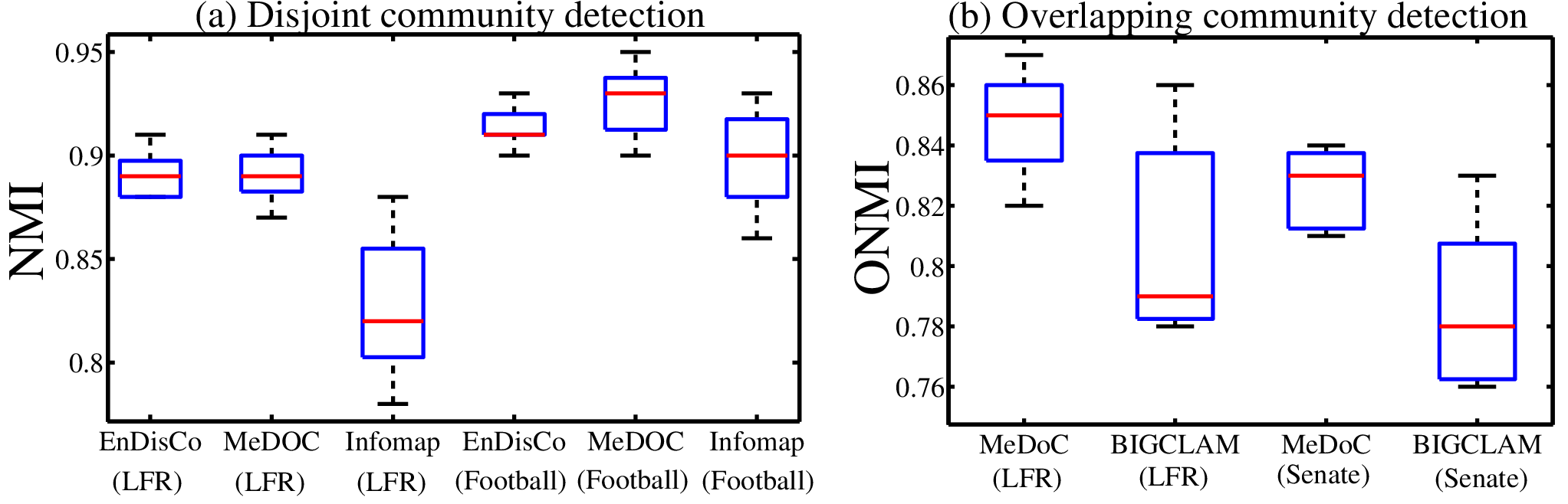
CD algorithms suffer from the problem of “degeneracy of solutions” [11] which states that an optimization algorithm can produce exponentially many solutions with (nearly-)similar optimal value of the objective function (such as modularity); however the solutions may be structurally distinct from each other. Figure 1 showed how InfoMap produces many outputs for different vertex orderings of Football network. We test this by considering the default LFR network and one real-world network (Appendix [1] shows results on more real world networks) and run the algorithms on different vertex orderings of each network. We then measure the pair-wise similarity of the solutions obtained from each algorithm. The box plots in Figure 5 show the variation of the solutions for EnDisCo, MeDOC and the best baseline algorithm in both disjoint and overlapping community detections. We observe that the median similarity is high with EnDisCo and MeDOC and the variation is comparatively small. These results suggest that our algorithms provide more robust results than past work and alleviate the problem of degeneracy of solutions.
IX Conclusion
In this paper, we proposed two general frameworks for ensemble community detection. EnDisCo identifies disjoint community structures, while MeDOC detects both disjoint and overlapping community structures. We tested both algorithms on both synthetic data using the LFR benchmark and with several real-world datasets that have associated ground-truth community structure. We show that both EnDisCo and MeDOC are more accurate than existing CD algorithms, though of course, EnDisCo and MeDOC leverage them. We further show that for disjoint CD problems, EnDisCo and MeDOC both beat a well known existing disjoint ensemble method called consensus clustering [20] – both in terms of accuracy (measured via both Normalized Mutual Information and Adjusted Rand Index) and run-time. To our knowledge, MeDOC is the first ensemble algorithm for overlapping community detection that we have seen in the literature. In future, we would like to develop theoretical explanation to justify the superiority of ensemble approaches compared to the discrete models. Other future direction could be to make the ensemble frameworks parallelized. We will apply the proposed methods to identify communities in specific datasets, such as malware traces, protein interaction networks etc.
Acknowledgment
Parts of this work were funded by ARO Grants W911NF-16-1-0342, W911NF1110344, W911NF1410358, by ONR Grant N00014-13-1-0703, and Maryland Procurement Office under Contract No. H98230-14-C-0137.
References
- [1] http://www.umiacs.umd.edu/~tanchak/Appendix.pdf.
- [2] V. D. Blondel, J.-L. Guillaume, R. Lambiotte, and E. Lefebvre, “Fast unfolding of communities in large networks,” JSTAT, p. P10008, 2008.
- [3] T. Chakraborty, “Leveraging disjoint communities for detecting overlapping community structure,” Journal of Statistical Mechanics: Theory and Experiment, vol. 2015, no. 5, p. P05017, 2015.
- [4] T. Chakraborty, S. Sikdar, N. Ganguly, and A. Mukherjee, “Citation interactions among computer science fields: a quantitative route to the rise and fall of scientific research,” Social Netw. Analys. Mining, vol. 4, no. 1, p. 187, 2014.
- [5] T. Chakraborty, S. Sikdar, V. Tammana, N. Ganguly, and A. Mukherjee, “Computer science fields as ground-truth communities: their impact, rise and fall,” in ASONAM, Niagara Falls, Canada, 2013, pp. 426–433.
- [6] T. Chakraborty, S. Srinivasan, N. Ganguly, A. Mukherjee, and S. Bhowmick, “On the permanence of vertices in network communities,” in SIGKDD, New York, USA, 2014, pp. 1396–1405.
- [7] A. Clauset, M. E. J. Newman, , and C. Moore, “Finding community structure in very large networks,” Phy. Rev. E., vol. 70, no. 6, p. 066111, 2004.
- [8] J. Dahlin and P. Svenson, “Ensemble approaches for improving community detection methods.” CoRR, vol. abs/1309.0242, 2013.
- [9] L. Danon, A. Diaz-Guilera, J. Duch, and A. Arenas, “Comparing community structure identification,” JSTAT, vol. 9, p. P09008, 2005.
- [10] S. Fortunato, “Community detection in graphs,” Physics Reports, vol. 486, no. 3-5, pp. 75 – 174, 2010.
- [11] B. Good, Y. D. Montjoye, and A. Clauset, “Performance of modularity maximization in practical contexts,” Phy. Rev. E., vol. 81, no. 4, p. 046106, 2010.
- [12] S. Gregory, “Finding overlapping communities in networks by label propagation,” New J. Phys., vol. 12, no. 10, p. 103018, 2010.
- [13] K. C. H. Shen, X. Cheng and M. B. Hu, “Detect overlapping and hierarchical community structure in networks,” Physica A, vol. 388, no. 8, pp. 1706–1712, 2009.
- [14] L. Hubert and P. Arabie, “Comparing partitions,” Journal of classification, vol. 2, no. 1, pp. 193–218, 1985.
- [15] L. G. S. Jeub, P. Balachandran, M. A. Porter, P. J. Mucha, and M. W. Mahoney, “Think locally, act locally: Detection of small, medium-sized, and large communities in large networks,” Phy. Rev. E., vol. 91, p. 012821, 2015.
- [16] R. Kanawati, “Yasca: An ensemble-based approach for community detection in complex networks,” in COCOON. Cham: Springer, 2014, pp. 657–666.
- [17] ——, “Ensemble selection for community detection in complex networks,” in SCSM. CA, USA: Springer, 2015, pp. 138–147.
- [18] A. Lancichinetti, F. Radicchi, J. J. Ramasco, and S. Fortunato, “Finding statistically significant communities in networks,” PLoS ONE, vol. 6, no. 4, p. e18961, 2011.
- [19] A. Lancichinetti and S. Fortunato, “Benchmarks for testing community detection algorithms on directed and weighted graphs with overlapping communities,” Phy. Rev. E, vol. 80, p. 016118, 2009.
- [20] ——, “Consensus clustering in complex networks,” Nature Scientific Reports, vol. 2, 2012.
- [21] A. McDaid and N. Hurley, “Detecting highly overlapping communities with model-based overlapping seed expansion,” in ASONAM, Washington, DC, USA, 2010, pp. 112–119.
- [22] A. F. McDaid, D. Greene, and N. J. Hurley, “Normalized mutual information to evaluate overlapping community finding algorithms,” CoRR, vol. abs/1110.2515, 2011.
- [23] T. Nepusz, A. Petróczi, L. Négyessy, and F. Bazsó, “Fuzzy communities and the concept of bridgeness in complex networks,” Phy. Rev. E., vol. 77, p. 016107, 2008.
- [24] M. E. Newman, “Modularity and community structure in networks,” PNAS, vol. 103, no. 23, pp. 8577–8582, 2006.
- [25] M. E. J. Newman, “Fast algorithm for detecting community structure in networks,” Phy. Rev. E., vol. 69, no. 6, p. 066133, Jun. 2004.
- [26] M. Ovelgönne and A. Geyer-Schulz, “An ensemble learning strategy for graph clustering,” in Graph Partitioning and Graph Clustering, ser. Contemporary Mathematics, vol. 588, pp. 187–206.
- [27] G. Palla, I. J. Farkas, P. Pollner, I. Derényi, and T. Vicsek, “Fundamental statistical features and self-similar properties of tagged networks,” New J. Phys., vol. 10, no. 12, p. 123026, 2008.
- [28] P. Pons and M. Latapy, “Computing communities in large networks using random walks,” J. Graph Algorithms Appl., vol. 10, no. 2, pp. 191–218, 2006.
- [29] U. N. Raghavan, R. Albert, and S. Kumara, “Near linear time algorithm to detect community structures in large-scale networks,” Phy. Rev. E., vol. 76, no. 3, 2007.
- [30] M. Rosvall and C. T. Bergstrom, “Maps of random walks on complex networks reveal community structure,” PNAS, vol. 105, no. 4, pp. 1118–1123, 2008.
- [31] X. Wang, L. Tang, H. Liu, and L. Wang, “Learning with multi-resolution overlapping communities,” Knowl. Inf. Syst., vol. 36, no. 2, pp. 517–535, 2013.
- [32] J. Xie and B. K. Szymanski, “Towards linear time overlapping community detection in social networks,” in PAKDD, Malaysia, 2012, pp. 25–36.
- [33] R. Xu and D. Wunsch, II, “Survey of clustering algorithms,” Trans. Neur. Netw., vol. 16, no. 3, pp. 645–678, May 2005.
- [34] J. Yang and J. Leskovec, “Overlapping community detection at scale: A nonnegative matrix factorization approach,” in WSDM. New York, USA: ACM, 2013, pp. 587–596.