Cubic Planar Graphs and Legendrian Surface Theory

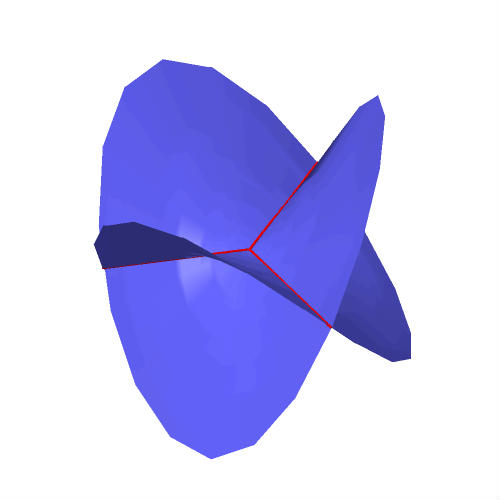
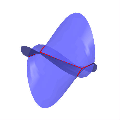
Our Legendrian surfaces lie in an open domain of $S^{5}$ contactomorphic to the cosphere bundle $T^{\infty}\mathbf{R}^{3}$ and to the jet bundle $J^{1}(S^{2})$. They are genus-$g$ surfaces double-covering their base projection to $S^{2}$ with $2g+2$ branch points. Such a Legendrian $S$ can be defined from a cubic planar graph $\Gamma\subset S^{2}$, by constructing a wavefront projection of $S$ in $S^{2}\times\mathbf{R}\cong\mathbf{R}^{3}\setminus\{0\}$ that is generically two-to-one over the base projection to $S^{2}$, but one-to-one over $\Gamma.$ (The original $S,$ not just its wavefront, is in fact still $2:1$ over the edges and only $1:1$ over the $2g+2$ vertices.)

In this introduction, we will mainly restrict our attention to simple (no loops or multiple edges) cubic planar graphs, although the Legendrian surface associated to $\Gamma$ is of interest more generally.

Given such a Legendrian $S\subset T^{\infty}\mathbf{R}^{3}$ we can take it as singular-support data for a category of constructible sheaves. This category of constructible sheaves is equivalent [NZ, N] to a Fukaya category in $T^{*}\mathbf{R}^{3}$ with asymptotic conditions on geometric branes defined by $S$. We give an explicit description of the moduli space $\mathcal{M}_{r}$ of objects of this category that have microlocal rank $r$, focusing on $\mathcal{M}:=\mathcal{M}_{1}.$ In [KS], sheaves in $\mathcal{M}_{r}$ are called “pure,” or “simple” if $r=1$. In the Fukaya category, points of $\mathcal{M}_{r}$ correspond to stacks of $r$ basic branes ending on $S$ — see Remark 1.5.

A point of $\mathcal{M}$ is easy to describe: think of the faces of $\Gamma$ as countries on a map of the globe $S^{2},$ and color each one with a point in $\mathbf{P}^{1}$ so that countries which share an edge border have different colors. The set of such choices provides a framed version of the moduli space: to get $\mathcal{M}$, we must quotient by the automorphism group $\mathrm{PGL}_{2}$ of $\mathbf{P}^{1}$, which acts freely. If we put $\widehat{\Gamma}$ for the dual graph, this means $\mathcal{M}$ is the set of graph colorings of $\widehat{\Gamma},$ with colors chosen in $\mathbf{P}^{1},$ modulo $\mathrm{PGL}_{2}$. As a variety, $\mathcal{M}$ is defined over the integers and we may count its points over finite fields:

It is known [B] that if $G$ has $n$ vertices and $e$ edges, then $P_{G}(x)=x^{n}-ex^{n-1}+O(x^{n-2}).$ If $\Gamma$ is a cubic planar graph with $v$ vertices, $e$ edges and $f$ faces, then it is easy to show that

where $g$ is the genus of the corresponding Legendrian surface $S.$

Nevertheless, we can construct smooth fillings that are not exact. Suppose that $\Gamma$ is drawn on the surface of the ball $D^{3}$. A foam filling $\Gamma$ is a singular surface $\mathbf{F}\subset D^{3}$ with codimension-one singularities that look like the letter “Y” times an interval, and codimension-two singularities (points) that look like the cone over the $1$-skeleton of a tetrahedron, and such that $\mathbf{F}\cap\partial D^{3}=\Gamma.$

A foam is the same combinatorial structure that configurations of soap bubbles have — the singularities are the Plateau borders of the soap film. It is interesting to speculate whether, if we were to impose Plateau’s laws on the foam (that the sheets of soap have constant mean curvature and meet at equilateral angles), the Lagrangian we construct could be chosen to be sLags. The singular Lagrangians are easy to describe, they are branched double covers of the $1$-skeleton of the foam. The smooth Lagrangians we construct are not just non-exact but obstructed: they are not objects in a Fukaya category if one does not introduce a “bounding cochain.”

In any case, there is a map from $\mathcal{M}$ that corresponds to “restrict a local system to its boundary” when an exact Lagrangian does exists, and makes sense over the whole moduli space. It is a special case of the $\mu\mathit{hom}$-functor of [KS], that was called “microlocal monodromy” in [STZ2]. This map

is isomorphic to one considered in [DGG1], and is known to be Lagrangian with respect to the symplectic structure on $H^{1}(S,\mathbf{C}^{*})$ induced by the intersection form — something that follows in this sheaf-theoretic context from the general results of [BD, ST1].

Recall that Aganagic-Vafa [AV] fix a Lagrangian brane, then use the equation of the moduli space of that brane in the resolved conifold to define conjectural open Gromov-Witten invariants. In [AKV] the construction was extended to different “phases” and “framings” of the brane, and to other toric Calabi-Yau three-folds, including $\mathbf{C}^{3}.$ In [AV3] the authors apply this construction to conormals of knots and call this “generalized SYZ mirror symmetry.” Our method generalizes this technique to three-dimensional branes that look nothing like tori, so we refer to it as “generalized AV mirror symmetry.”

The original AV construction identifies a distinguished set of coordinates $x=e^{u},y=e^{v}$ on an ambient symplectic $(\mathbf{C}^{*})^{2}$ and uses the equation of the moduli space $F(u,v)=0$ to solve $v=-\partial_{u}W$ (the choice of sign is historical), where $W$ has a four-dimensional interpretation as a superpotential, but also as the generating function for open disk invariants. The procedure depends on a choice of “framing” which distinguishes the second coordinate, as the so-called “phase” only identifies one of the two.

The method can be interpreted in the following way. The moduli space $\mathcal{M}$ of the brane is a Lagrangian submanifold in $H^{1}(S,\mathbf{C}^{*})=(\mathbf{C}^{*})^{2g}$. A phase is a geometric Lagrangian, an oriented $3$-manifold $L$, contained in $\mathbf{R}^{6}$ with boundary on $S$. A phase determines a Lagrangian map $H^{1}(L,\mathbf{C}^{*})\to H^{1}(S,\mathbf{C}^{*})$, and we define a framing to be an extension of this to a symplectic map $T^{*}H^{1}(L,\mathbf{C}^{*})\to H^{1}(S,\mathbf{C}^{*})$. Then it makes sense to try to express $\mathcal{M}$ as the graph of the differential of a multivalued transcendental function $W:H^{1}(L,\mathbf{C}^{*})\to\mathbf{C}$.

We conjecture that $W$ is the generating function of open Gromov-Witten disk invariants.

Currently, the Lagrangians considered in this paper fall outside the limited class for which open Gromov-Witten invariants are rigorously defined, so the conjecture is not strictly precise as it stands. However, there is recent progress in the work of Solomon and Tukachinsky — see Remark 4.7. Meanwhile, we can make a precise integrality conjecture, following Ooguri-Vafa [OV]:

There are integers $a(d,f)\in\mathbf{Z}$ and an order-two element $\varepsilon_{f}\in H^{1}(L,\mathbf{C}^{*})$, indexed by homology classes $d\in H_{1}(L,\mathbf{Z})$ and a framing $f$, such that

(1.2.1)

$$W(x)=\sum_{d}a(d,f)\mathrm{Li}_{2}\left((\varepsilon_{f}x)^{d}\right)$$

where $(-)^{d}$ denotes the monomial function $H^{1}(L,\mathbf{C}^{*})\to\mathbf{C}$ corresponding to $d$ and $\mathrm{Li}_{2}(z)=\sum\frac{1}{n^{2}}z^{n}$ is the classical dilogarithm function.

Identities involving $\mathrm{Li}_{2}(z)$, $\mathrm{Li}_{2}(1/z)$, and other arguments related by Möbius transformations prevent equation (1.2.1) from determining $a(d,f)$ uniqely. We expect that by restricting the sum to a strictly convex (“Mori”) cone of elements in $H_{1}(L,\mathbf{Z})$ that support holomorphic disks, the coefficients $a(d,f)$ become uniquely determined and are the physical BPS numbers. The translation by $\varepsilon_{f}$ functions as a kind of mirror map (change of variables to write superpotential correctly), that we do not have a great explanation for.

Before giving some examples let us discuss coordinates. The choice of phase allows us to choose coordinates $(v_{1},\ldots,v_{g})$ on the universal cover of $H^{1}(S,\mathbf{C}^{*})$ that cut out $H^{1}(L,\mathbf{C})$, and a framing nails down conjugate coordinates $u=(u_{1},...,u_{g})$. These choices identify the universal cover with $\mathbf{C}^{2g}\cong T^{*}\mathbf{C}^{g}$, and $W$ is the solution to $v_{i}=\pm\partial_{u_{i}}W$.

We implement this generalized AV mirror symmetry explicitly in several examples.

• •

  When $\Gamma$ is the complete graph with four vertices, we have $f=g+3=4,$ so $g=1$ and the filling is a solid torus. It is the Aganagic-Vafa brane in $\mathbf{C}^{3}$. Then $\mathcal{M}\subset(\mathbf{C}^{*})^{2}$ is defined by

  $$x+y=1,$$

  a pair of pants, and here we have implicitly chosen a phase and (zero) framing to write $x=e^{u},y=e^{v}.$ Then $v=-\partial_{u}W$ identifies $W={\rm Li}_{2}(x):=\sum_{n>0}\frac{1}{n^{2}}x^{n}$, as in the work of Aganagic-Vafa [AV]. The procedure is identical to theirs in this example, so different framings — making the replacement $u\to u+pv$ — give the framing-dependent disk invariants computed by Aganagic-Klemm-Vafa [AKV, Section 6.1].

• •

  When $\Gamma$ is a triangular prism, $g=2$ and the moduli space $\mathcal{M}$ is cut out by two equations:

  $$x_{1}+y_{1}=1,\qquad x_{2}+y_{2}=1.$$

  Then $\mathcal{M}$ is a product of two copies of the pair of pants, and zero framing ($x_{i}=e^{u_{i}},y_{i}=e^{v_{i}}$) gives $W={\rm Li}_{2}(x_{1})+{\rm Li}_{2}(x_{2}).$ “Diagonal” framings $u_{1}\to u_{1}+p_{1}v_{1},\;u_{2}\to u_{2}+p_{2}v_{2}$ lead to different BPS numbers, but exactly as above. Here, however, we also have the possibility of non-diagonal framings such as

  $$u_{1}\to u_{1}+pv_{2},\qquad u_{2}\to u_{2}+pv_{1}.$$

  For example, when $p=1$ we find $W(x_{1},x_{2})={\rm Li}_{2}(x_{1})+{\rm Li}_{2}(x_{2})-{\rm Li}_{2}(x_{1}x_{2}).$ More generally, framings are determined by a symmetric $2\times 2$ integer matrix $M_{i}{}^{j}$ via $u_{i}\to u_{i}+M_{i}{}^{j}v_{j}.$ We consider these examples in Section 5.3. While we generally cannot write the superpotential $W$ in closed form, we can perform strict integrality checks: in all cases considered, we derive integer BPS numbers $a(d,f)$ using the Ooguri-Vafa $1/d^{2}$ multiple cover formula [OV].

• •

  When $\Gamma$ is the union of vertices and edges of a cube, $g=3$ and we can similarly define multi-coordinates $(u,v)$ for $\mathbf{C}^{6}\cong T^{*}\mathbf{C}^{3}_{u}$. Then (the universal cover of) $\mathcal{M}$ is a graph of $-dW(u),$ where

  $$W={\rm Li}_{2}(x_{1})+{\rm Li}_{2}(x_{2})+{\rm Li}_{2}(x_{3})-{\rm Li}_{2}(x_{1}x_{2})-{\rm Li}_{2}(x_{1}x_{3}),$$

  with $x_{i}=e^{-u_{i}}.$ The answer is written in terms of integer linear combinations of dilogarithms, meaning the conjectural disk invariants obey integrality.

While preparing this document, we learned of prior constructions with signifcant overlap to our own. We will try to explain the connections, similarities and differences to the present work. While the works in Section 1.4.2 appeared first, we describe the relations in reverse chronological order due to the greater similarity in the approach of the latter works.

In [STZ2, §2.2.1], we associated to each front diagram $\Phi\subset\mathbf{R}^{2}$ a Legendrian graph $\Lambda^{+}$, obtained from the Legendrian lift $\Lambda$ of $\Phi$ by attaching a Legendrian chord joining the two points projecting to a crossing. The cone over $\Lambda^{+}$ is the smallest Lagrangian containing the cone over $\Lambda$ that is closed under addition. (Thus $\Lambda^{+}$ is “cragged” in the language of [SS].)

We may consider a similar extended form of $S$, which we denote by $S^{+}$. If $i$ is an edge of $\Gamma$, its preimage is parametrized by a circle $\gamma_{i}:S^{1}\to S$, with a distinguished orientation we discuss in §4.6. If the edge $i$ is not a loop, then $\gamma_{i}$ is an embedded circle, while if $i$ is a loop from vertex $v$ to itself, $\gamma_{i}$ is an immersion with a single double point at $\pi^{-1}(v)$. We attach a Legendrian disk to $S$ whose boundary is along $\gamma_{i}$.

To define $D_{i}$, first note that each point $p$ along $i$ has two associated outward conormal rays, one along each branch of the wavefront immersion. $D_{i}$ is the subset of the cosphere bundle over $i$ which, at a point $p\in i$, consists of the acute angle of the conormal rays between those two. Note this angle shrinks to zero at the endpoints of $i$, where $D_{i}$ is just a point. Thus $D_{i}$ is the disk formed by the family of intervals over the interval $i,$ collapsing at the boundary.

If $i$ is an edge of $\Gamma$ that is not a loop, we may construct a new graph $\Gamma^{\prime}$ by changing $\Gamma$ in a neighborhood of $i$ according to the following diagram

The faces of $\Gamma$ and of $\Gamma^{\prime}$ are in natural bijection with each other. By performing this move at different edges one can get from any graph to any other graph. Indeed this is the sense in which cubic planar graphs label the top-dimensional cells in the Harer-Penner-Mumford-Thurston complex for $M_{0,n}$, which is connected.

Let $U_{i}\subset S^{2}$ be a neighborhood of $i$. If $i$ is not a loop, the preimage of $U_{i}$ in $S$ is an annulus, and its preimage in $S^{+}$ is an annulus with a disk attached — let us denote them by $A$ and $A^{+}$. The Lagrangian projection of $A^{+}$ is an embedding into $T^{*}U_{i}$ — it is an exact, singular Lagrangian of the kind that has been considered by [Y]. Yau considers a “disk move” which is part of our model for cluster transformations in [STWZ, STW]. In the present context these are related:

The two exact Lagrangian surfaces on either side of a disk move are part of the “focus-focus” family of Lagrangian annuli:

In particular the Legendrians $S$ must have the same classical invariants.

Let $n$ be an integer, which for simplicity we will assume is odd. Let $\Lambda\subset S^{3}$ be a Legendrian $(2,n)$-torus knot. Two families of $\frac{1}{n+1}\binom{2n}{n}$ exact Lagrangian fillings of $\Lambda$ have been produced, first in [EHK] and later in [STWZ]. Roughly speaking, [EHK] produces this family of fillings by a “elementary Lagrangian cobordism” technique, and [STWZ] by an “alternating strand diagram” technique. We sketch here a third construction of a family of $\frac{1}{n+1}\binom{2n}{n}$ fillings, in terms of hyperelliptic wavefronts, and an equivalence between these fillings and the EHK fillings.

The building-block example of a foam, is the cone over the $1$-skeleton of a regular tetrahedron centered at the origin. Before turning to our general construction let us explain the relationship between this foam and the Harvey-Lawson cone. This is the Lagrangian subset $\mathit{HL}\subset\mathbf{C}^{3}$ given parametrically by

where $r\geq 0$ and $(s,t)\in S^{1}\times S^{1}.$ It is a cone over a two-torus, with a conic singularity at the origin $r=0$. Coordinatize $\mathbf{C}^{3}$ as $z=x+iy,$ with $z=(z_{1},z_{2},z_{3})$ and likewise for $x$ and $y$. Then $\mathit{HL}$ is special Lagrangian with respect to the standard Calabi-Yau structure. Define $n=\frac{x}{|x|}\in S^{2}$ and $f=n\cdot y\in\mathbf{R}$ The restriction of ${\mathit{H}L}$ to fixed $r$ is Legendrian, with wavefront projection

shown in Figure 2.0.1. The Harvey-Lawson cone is therefore a singular Lagrangian filling of the Legendrian surface associated to the tetrahedron. (It is also exact and special.)

We will be interested here in a different projection, to the real three-space:

This is a double cover branched over the four rays

Note the generator for the $\mathbf{Z}/2$ Galois group of this covering is given explicitly by $(r,s,t)\mapsto(r,-s,-t)$. The unusually low dimension of the critical value locus — here it has codimension $2$ — is related to the fact that both $\mathit{HL}$ and the kernel of the projection $\mathbf{C}^{3}\to\mathbf{R}^{3}$ are special Lagrangian of the same phase.

The rays (3.1.1) are generated by the vertices of a regular tetrahedron. The foam whose walls are the sectors through these edges play a role in the exactness of $\mathit{HL}$. Indeed being a cone, the set $\mathit{HL}$ is contractible and therefore an exact Lagrangian with respect to any primitive $\alpha$ for $\omega$. It is natural to take for $\alpha$ the canonical one-form obtained when identifying $\mathbf{C}^{3}$ with $T^{*}\mathbf{R}^{3}$. Then we compute $\alpha|_{\mathit{HL}}=df$ where

Note that $f=0$ precisely when $(x_{1},x_{2},x_{3})$ are in walls of the tetrahedral foam.

Let $\Gamma\subset S^{2}$ be a cubic planar graph and let $\mathbf{F}\subset D^{3}$ be a foam whose boundary is $\Gamma$. Let $\pi:L(\mathbf{F})\to D^{3}$ denote the connected double cover branched over the $1$-skeleton of $\mathbf{F}$, and write $\iota_{L(\mathbf{F})}$ for its nontrivial Deck transformation. Then $L(\mathbf{F})$ is a manifold away from the vertices of $\mathbf{F}$ — near each vertex it is diffeomorphic to the Harvey-Lawson cone. The boundary of $L(\mathbf{F})$ is naturally identified with the hyperelliptic surface $S$ branched over the vertices of $\Gamma$.

We choose a function $z:L(\mathbf{F})\to\mathbf{R}$ that is smooth away from the cone points of $L(\mathbf{F})$, that is odd for the Deck transformation of $\pi$ (i.e. $z\circ\iota=-z$) and that has the following additional properties:

1. (1)

   In a neighborhood $U$ of each cone point, there are coordinates on $\pi^{-1}(U)$ such that $z|_{U}$ looks like (3.1.2)

2. (2)

   The only critical points of $z$ are on $\pi^{-1}(\mathbf{F}^{1})$, i.e. on the critical points of $\pi$. Furthermore, in a collar neighborhood of $\partial D^{3}$, $z$ is linear along each ray.

Then (just as in §2.3, but one dimension up) we obtain an exact Lagrangian in $T^{*}D^{3}$ by taking $(\pi,\nabla z)$ whose restriction to $T^{*}D^{3}|_{\partial D^{3}}\cong(T^{*}S^{2})\times\mathbf{R}$ is Legendrian. For example, the function $f$ of Remark 3.2 has almost all of these properties, except that it is quadratic instead of linear along each ray. We obtain a function $z$ by damping $f$ with an exponent that smoothly interpolates between $1$ and $1/2$.

An exact filling of $S$ is an exact Lagrangian cobordism from $S$ to the empty Legendrian. One can ask whether these cobordisms can be factored into simpler cobordisms — as we discussed in §2.3, this is how Ekholm, Honda, and Kálmán discovered their Lagrangians. In this section we indicate a (somewhat) analogous description of the singular exact fillings of §3.2, in particular by rough analogy with the discussion of §2.3.3, but the analogy highlights some differences.

Suppose that $\Gamma$ has no self-loops or multiple edges, so its planar dual graph $\hat{\Gamma}$ is a triangulation of $S^{2}$. Just as a cubic planar tree is dual to an ideal triangulation of a disk, an ideal foam is dual to an ideal “tetahedronation” of the ball $D^{3}$ that restricts to $\hat{\Gamma}$ on $\partial D^{3}=S^{2}$. Thus if $\mathbf{F}$ is a foam filling of $\Gamma$, let $\hat{\mathbf{F}}$ be the dual tetrahedronation restricting to $\hat{\Gamma}$ on the boundary. If $\mathbf{F}$ is an ideal foam, $\hat{\mathbf{F}}$ is an ideal triangulation: it has no vertices besides those on $\partial D^{3}$. For simplicity, we assume $\hat{\mathbf{F}}$ is shellable, but as in the two-dimensional case (see Remark 2.4) this assumption is unnecessary and $L(\mathbf{F})$ depends only on the foam $\mathbf{F}$.

In §2.3.3 we noted that a shelling of the triangles in the dual triangulation of a disk gives an “EHK factorization” of the exact Lagrangian surfaces into elementary cobordisms. Thus, let $n$ be the number of tetrahedra in $\hat{\mathbf{F}}$, equivalently the number of interior vertices in $\mathbf{F}$, and let $a_{n},a_{n-1},\ldots,a_{1}$ be a shelling of the tetrahedra in $\hat{\mathbf{F}}$. (We use descending indices to better match the notation of §2.3.3; the highest index is the outer shell.) For each $k,$ the union of $a_{n},\ldots,a_{n-k}$ is another polyhedron with a tetrahedronation — it is dual to a foam filling $\mathbf{F}(k)$ with boundary a cubic planar graph $\Gamma(k)$. Write $L(\mathbf{F}(k))$ for the singular exact Lagrangian double cover branched over the one-skeleton of $\mathbf{F}(k)$. We will indicate how $L(\mathbf{F}(k+1))$ is obtained from $L(\mathbf{F}(k))$ and a Harvey-Lawson-type Lagrangian $\mathit{HL}_{k+1}$ by gluing $L(\mathbf{F}(k))$ and $\mathit{HL}_{k+1}$ along parts of their boundaries.

For $\mathit{HL}_{k+1}$, we take the branched double cover of the one-skeleton of the foam associated with a small tetrahedron with one vertex on each face of $a_{n-(k+1)}$. There are two cases to consider: the tetrahedron $a_{n-(k+1)}$ is incident with $\bigcup_{i=1}^{k}a_{n-i}$ along either exactly one or exactly two of its faces. (Since we assume $\hat{\mathbf{F}}$ has no internal vertices, it is impossible for $a_{n-(k+1)}$ to be indicent with the previous simplices along three of its faces.)

If it is incident along exactly one face, the left-hand figure illustrates $L(\mathbf{F}(k))\cup\mathit{HL}_{k+1}$ before the gluing, and the right-hand figure illustrates it after the gluing:

To understand the case of an interior face of ${\bf F}$, i.e. edge of $\hat{\bf F}$, consider Figure 3.3.2 below.

To define $\mathbf{F}(k+1)$ and obtain from it a singular exact filliing, we construct a cobordism from the boundary of $L(\mathbf{F}(k))\sqcup HL_{k+1}$ to a new space by modifying the wavefront to remove the spurious blue loop. Consider a neighborhood of the blue loop in the front projection. It is a cylinder. The cobordism takes this cylinder to two disks, just like the two-to-one-sheet hyperboloid cobordism $x^{2}+y^{2}-z^{2}=t,\;t\in[0,1]$. Afterward, the blue loop disappears and the red edges make up a new polytope, or dually define $\mathbf{F}(k+1)$, which in Figure 3.3.2 is a triangular prism.

The one-skeleton $\mathbf{F}^{1}$ of a foam $\mathbf{F}\subset D^{3}$ is a kind of singular tangle in the ball, joining the vertices of graph on the boundary. The singularities are at the internal vertices $\mathbf{F}^{0}$ of the foam, suppose that there are $T$ of these. Then we can associated as many as $3^{T}$ smoothings of this singular tangle, as follows. In a neighborhood of each of the $T$ vertices, choose coordinates in which $\mathbf{F}^{1}$ looks like the rays of (3.1.1), and replace $\mathbf{F}^{1}$ by one of the smooth hyperbolas

where $i_{1},i_{2},i_{3}$ is a permutation of $\{1,2,3\}$ — the hyperbola is determined just by the value of $i_{1}$. In fact, this is precisely the critical locus of the projection to $\mathbf{R}^{3}_{x}$ of the Harvey-Lawson smoothing, the solid torus of Example 3.7 below.

We have not investigated what kinds of tangles can appear, the examples we have encountered so far are all quite unlinked.

We have constructed singular exact fillings of $S$ with the topology of double covers of the ball, branched over $\mathbf{F}^{1}$, the edges of a foam. Example 3.7 below suggests that we search for smooth fillings with the topology of a double cover of the ball, branched over a tangle obtained by smoothing $\mathbf{F}^{1}$ in the sense of §3.4. However the example also suggests that such smoothings will not be exact. Theorem 4.4 gives a strong result making this precise. Let us therefore make some general remarks about nonexact fillings.

Let $(M,\omega=d\alpha)$ be an exact symplectic manifold. In the literature on Lagrangian fillings of Legendrians $\Lambda\subset\partial M$, the condition that the Lagrangian has conical ends is often imposed. For 3-dimensional Lagrangians, this has an undesirable consequence. If $L$ is $3$-dimensional and $U$ is a collar neighborhood of the boundary of $L$, the map $H^{1}(L,\mathbf{R})\to H^{1}(U,\mathbf{R})$ is often injective, so if $\alpha$ is exact on $U$, it is exact on all of $L$. This suggests that if we wish to consider non-exact Lagrangians, the condition that $L$ has conical ends is inappropriate. A notion of “asymptotically conical” might be more appropriate, as in [J, Def. 7.1] for special Lagrangians, or [NZ, Def. 5.4.1] for subanalytic Lagrangians.

If $\mathcal{T}$ is a tangle associated to a foam $\mathbf{F}$, write $\pi:L(\mathcal{T})\to D^{3}$ for the double cover branched over $\mathcal{T}$. In the rest of the paper we will refer to any Lagrangian map $L(\mathcal{T})\to T^{*}D^{3}$ whose projection to $D^{3}$ is $\pi$ as a “filling” of $S$ — or a “filling modeled on $\mathcal{T}$” — without heed for asymptotic conditions. Note that even so, the boundary of $L(\mathcal{T})$ is canonically identified with $S$, since $\mathcal{T}\cap\partial D^{3}$ is exactly the set of vertices of $\Gamma$. We also will not necessarily assume that the map $L(\mathcal{T})\to T^{*}D^{3}$ is an embedding.

Once a filling modeled on $\mathcal{T}$ is given, the pull-back of the canonical one-form on $T^{*}D^{3}$ to $L(\mathcal{T})$ is closed. Conversely, for each closed one-form there is at most one Lagrangian map $L(\mathcal{T})\to T^{*}D^{3}$ whose projection to $D^{3}$ is $\pi$.

To see that a filling modeled on $\mathcal{T}$ is determined by a $1$-form on $L(\mathcal{T})$, write $x_{1},x_{2},x_{3}$ for the coordinates on $D^{3}$, $y_{1},y_{2},y_{3}$ for the coordinates on $T^{*}D^{3}$, and let $s_{1},s_{2},s_{3}$ be local coordinates on $L(\mathcal{T})$. If $\alpha=\alpha_{1}ds_{1}+\alpha_{2}ds_{2}+\alpha_{3}ds_{3}$ is a closed one-form on $L(\mathcal{T})$, then $y_{1},y_{2},y_{3}$ are the solutions to $\sum y_{i}dx_{i}=\alpha$, which is equivalent to