Motion of charged particle in Reissner - Nordström spacetime:
A Jacobi metric approach

Point particle dynamics serves the important purpose of initiating the study more complex motion of extended bodies. A major area of interest, especially in recent times, is the motion of particles in the presence of black holes and naked singularities. The exhaustive topical works by Pugliese, Quevedo and Ruffini [1, 2] (as well as their series of earlier papers [3]) have revealed clearly the possibility of distinguishing between black holes and naked singularities in the case of charged particle dynamics in Reissner - Nordström background. The systematic analysis is based on the nature of particle motion for different charge to mass ratio in the Reissner - Nordström metric, (which is expected), but the non-trivial effect of the charge to mass ratio of the probe particle is indeed a surprising element. In this perspective, the aim of the present paper, dealing once again on the motion of point charge in the presence of a charged black hole, is not to add any more detail on the results of [1, 2, 4], but to compliment their observations and bring in new insights from an entirely different, (and hitherto less explored), point of view, that of Jacobi metric approach. This framework has generated a lot of interest after the series of works by Gibbons [5] and by Chanda, Gibbons and Guha [6].

The primary major difference is the following. On the one hand, Pugliese et.al. [1, 2, 3] relies on the covariant framework where geodesic motion takes place in Reissner-Nordström spacetime. The Lagrangian equation of motion is derived from the unrestricted variational principle with the charge and mass parameters of the source and probe dictating the particle motion for arbitrary particle energy, which is a derived quantity. On the other hand, in Jacobi metric framework, the equation of motion is obtained from a restricted variational principle with fixed energy where the Lagrangian depends on the Jacobi metric that involves the particle energy explicitly. Schematically for a system with $E=K-V$ where $E,K,V$ are total energy, kinetic energy and potential energy of a probe particle respectively, the Jacobi metric is given by

$$j=2(E-V)g$$

(1)

where $j$ is the Jacobi metric and $g$ the Riemannian metric on the manifold where the motion is taking place. In a sense each particle is performing geodesic motion in its own space(time). The Jacobi metric is manifestly non-covariant (on a spatial slice) [5, 6] and the equation of motion is derived from a restricted (Maupertuis) variational principle with fixed particle energy. Hence energy acts as an additional parameter along with the charge and mass parameters. The particle motion is still geodesic in the Jacobi metric space. (The fact that Jacobi metric is degenerate at the boundary where $E=V$ can create complications. For a detailed analysis on this issue and on ways of overcoming it, see for example [7].)

A novelty in our analysis is the associated (Gaussian) curvature corresponding to the Jacobi metric, in line with [5]. In the next section we will see that even dynamics in flat space can give rise to an effective non-zero curvature from Jacobi metric space. In fact trajectories can be classified according to the sign of the curvature: positive, negative and zero curvature (for Jacobi metric) corresponds to elliptic (with negative energy), hyperbolic (positive energy) and parabolic (zero energy) orbits respectively.

Apart from the importance of curvature in the Jacobi metric, one way in which the present work can compliment the exhaustive analysis of [1, 2] is the following: whereas [1, 2] relies on extremely detailed graphical analysis of the orbit structure keeping exact expressions we have provided analytic expressions of the orbits, albeit in a perturbative framework (of small charge of both the black hole and the probe). Also, compared to [1, 2] we have not restricted the analysis to circular orbits only.

We conclude this brief introduction by mentioning structure of the present work. The paper is organized as follows: In Section 2 we discuss generalities related to Maupertuis principle and Jacobi metric as well as its application in problems of particle dynamics in black hole spacetimes. Section 3 deals with the neutral massive particle motion in Reissner - Nordström background. Section 4 constitutes the study of motion of charged massive particle in Reissner - Nordström background. In Section 5 we provide a detailed analysis of Gaussian curvature for Jacobi metrics in the cases under study. The paper ends with our conclusions in Section 6. Detailed results are given Appendices 7 and 8.

The Maupertuis transformation and the associated Jacobi metric approach has generated a lot of recent interest [5, 6]. To understand the context let us start by considering an obvious fact that a curve can be parameterized in infinite number of ways (see for example [8] for a detailed discussion). For example, an ellipse

$$\frac{x^{2}}{a^{2}}+\frac{y^{2}}{b^{2}}=1$$

(2)

can be parameterized by

$$x=a~sin(t),~~y=b~cos(t),$$

(3)

and also by a different parameter $\tilde{t}$ related to $t$ by

$$\tilde{t}=(a^{2}+b^{2})t+(a^{2}-b^{2})sin(t).$$

(4)

Clearly the former parameterization (3) is connected to a two dimensional oscillator whereas the latter (4) is related to the Kepler problem. Generically the same trajectory can be attributed to distinct integrable systems where the parameter $t$ plays the role of time variable, conjugate to the respective Hamiltonian. Hence the question is how to derive the particular parameterization that matches with a known or interesting problem. The Maupertuis principle recasts this problem in a dynamical setup. The Maupertuis variational principle states that, given an $n$-dimensional configuration space Lagrangian $L(q_{i},\dot{q}_{i})$, extremals of the action

$$S=\int dt~L(q_{i},\dot{q}_{i})$$

(5)

coincide with extremals of the reduced action in a $2n-1$-dimensional phase space that is a level set of the Hamiltonian function $H(q_{i},p_{i})=E$. Here $p_{i}$ constitute the conjugate momenta to $q_{i}$ and the variation takes place on a fixed energy ($E$) hypersurface. In a more explicit way let us suppose a natural Hamiltonian in a Riemanniam manifold with metric $g_{ij}$,

$$H(q,p)=T(q,p)+V(q)=g_{ij}(q)p_{i}p_{j}+V(q).$$

(6)

The trajectories for $H$ on a fixed energy smooth submanifold will coincide with trajectories of a new Hamiltonian $\tilde{H}$ given by

$$\tilde{H}(q,p)=\tilde{T}(q,p)=\frac{g_{ij}(q)}{E-V(q)}p_{i}p_{j},$$

(7)

along with a transformation of the parameters,

$$d\tilde{t}=(E-V(q))dt.$$

(8)

Together (7,8) constitute the Jacobi transformation. A scaling of the effective metric provides the Jacobi metric. The two major novelties and advantages of the Maupertuis-Jacobi framework are:
(i) The Hamiltonian $\tilde{H}$ yields geodesic motion. This allows one to treat a dynamical problem as geodesic motion and well known machinery of geodesic motion can be directly exploited.
(ii) The Maupertuis principle and subsequent Jacobi transformation preserve integrability that is under this map an integrable system with a natural Hamiltonian goes over to another integrable system in the same phase space. Thus this scheme provides a method to search for new integrable systems.
(iii) The Gaussian curvature induced by Jacobi metric allows one to classify the trajectories based on their energy since it appears explicitly in Jacobi metric.

For a generic Lagrangian of the form, (following the notation of [5])

$\displaystyle L=\frac{1}{2}m_{ij}(x)\dot{x^{i}}\dot{x^{j}}-V(x)$

(9)

it was shown by Jacobi that the constrained motion of a particle with energy $E$ is provided by geodesics of the rescaled metric

$\displaystyle j_{ij}dx^{i}dx^{j}=2(E-V)m_{ij}dx^{i}dx^{j}.$

(10)

It is interesting to observe that particle interactions can induce a curvature in the Jacobi metric through the potential function in an otherwise flat Newtonian space. One of the early workers in this topic was Pin [9] who considered many body systems and in particular showed that the Gaussian curvature of the Jacobi metric has opposite sign to the particle energy $E$ (non-relativistic, without the rest energy). In later times Gibbons and coworkers [10, 11] have considered the optical metric in various physical situations which is a closely related concept for massless particles. Discussions on Jacobi metric approach in modern perspective can be found in [12].

Again very recently the Jacobi metric formalism in relativistic scenario has been applied by Gibbons [5] in an elegant study of massive particle motion in Schwarzschild spacetime. In the present paper we closely follow and extend this work to massive particle motion in Reissner - Nordström background. Indeed, Jacobi metric for a more general metric, that is the Kerr-Newman, has been derived in [6] although the probe particle dynamics was not considered there. We consider both cases of the probe particle being neutral and charged. The results show a qualitative difference between the two cases since in the latter one needs to consider the additional Coulomb interaction term between the source and probe particle. For neutral particle the correction terms depend on $Q^{2}$, $Q$ being the charge of the black hole but interestingly for the charged probe correction terms involve $qQ$ terms as well, $q$ being charge of the particle, showing that the relative sign between the particle and black hole charge becomes important.

For the generic metric

$\displaystyle ds^{2}=-V^{2}dt^{2}+g_{ij}dx^{i}dx^{j}$

(11)

the action for a massive particle in this background can be written as,

$\displaystyle S=-m\int Ldt=-m\int dt\sqrt{V^{2}-g_{ij}\dot{x^{i}}\dot{x^{j}}}.$

(12)

The canonical momentum

$\displaystyle p_{i}=\frac{m\dot{x^{i}}}{\sqrt{V^{2}-g_{ij}\dot{x^{i}}\dot{x^{j}}}},$

(13)

leads to the Hamiltonian

$\displaystyle H=\sqrt{m^{2}V^{2}+V^{2}g^{ij}p_{i}p_{j}}.$

(14)

This provides the Hamilton-Jacobi equation for the geodesics, parameterized by the energy $E$,

$\displaystyle\sqrt{m^{2}V^{2}+V^{2}g^{ij}\partial^{i}S\partial_{j}S}=E$

(15)

where $p_{i}=\partial_{i}S$ . Finally, the Hamiltonian-Jacobi equation for geodesics of Jacobi-metric $j_{ij}$ is given by,

$\displaystyle\frac{1}{E^{2}-m^{2}V^{2}}f^{ij}\partial_{i}S\partial_{j}S=1$

(16)

where $j_{ij}$ is defined as

$\displaystyle j_{ij}dx^{i}dx^{j}=(E^{2}-m^{2}V^{2})V^{-2}g_{ij}dx^{i}dx^{j}.$

(17)

Infact $f_{ij}=V^{-2}g_{ij}$ turns out to be the optical or Fermat metric. For massless particles $(m=0)$ the Jacobi metric becomes equal to the Fermat metric modulo a factor of $E^{2}$ and subsequently the geodesics do not depend upon energy E. However in the massive case, $m\neq 0$, the geodesics are $E$-dependent.

Let us put our work in its proper perspective. The explicit results and observations of the present work are not entirely new. Some of these are discussed in the book by Chandrasekhar [13]. More recent and detailed studies are provided in [1, 2, 3, 14]. However we have revisited the system from the Jacobi metric point of view. The Jacobi metric construction for charged massive particle and the subsequent analysis is completely new. Furthermore in the present work the Gaussian curvature induced by the Jacobi metric plays an essential role since the motion is geodesic in nature. We have compared results computed from Gaussian curvature consideration (in Jacobi metric approach) with similar results obtained via conventional scheme. For the charged probe, the interplay between the gravitational and Coulomb forces proves to be interesting.

Reissner-Nordström metric is a spherically symmetric solution of the coupled Maxwell Einstein gravity. It represents a black hole with a mass M and a charge Q and is given by

$\displaystyle ds^{2}=-(1-\frac{2M}{r}+\frac{Q^{2}}{r^{2}})c^{2}dt^{2}+\frac{dr^{2}}{(1-\frac{2M}{r}+\frac{Q^{2}}{r^{2}})}+r^{2}d\theta^{2}+r^{2}\sin^{2}\theta d\phi^{2}.$

(18)

For $Q=0$ the Schwarzschild metric is recovered. As is well known it has two horizons at $r=r_{\pm}=M\pm{\sqrt{M^{2}-Q^{2}}}$. The nature of the horizon singularities are different in Reissner - Nordström and Schwarzschild geometries. The latter is spacelike whereas the former is timelike and thus yielding richer possibilities regarding the nature of trajectories. There are timelike worldlines for particles that can cross $r_{+}$ horizon and skirting the singularity can move out to another spacetime region after crossing $r_{-}$. On the contrary for Schwarzschild geometry, after crossing the event horizon at $r=2M$ the particle has no option but to fall towards the singularity. The $r_{+}$-horizon acts like the $r=2M$ event horizon of Schwarzschild whereas $r_{-}$-horizon is termed as the Cauchy horizon.

Now, generalizing the result of Gibbons [5], the Jacobi metric corresponding to Reissner - Nordström solution is

$\displaystyle ds^{2}=(E^{2}-m^{2}+\frac{2Mm^{2}}{r}-\frac{Q^{2}m^{2}}{r^{2}})[\frac{dr^{2}}{(1-\frac{2M}{r}+\frac{Q^{2}}{r^{2}})^{2}}+\frac{r^{2}d\theta^{2}+r^{2}\sin^{2}\theta d\phi^{2}}{(1-\frac{2M}{r}+\frac{Q^{2}}{r^{2}})}]$

(19)

The first part is the conformal factor whereas the second factor is the optical metric. Due to spherical symmetry, we are allowed to study the system in the equatorial plane $\theta=\frac{\pi}{2}$ without any loss of generality. This reduces the Jacobi metric to the form,

$\displaystyle ds^{2}=(E^{2}-m^{2}+\frac{2Mm^{2}}{r}-\frac{Q^{2}m^{2}}{r^{2}})[\frac{dr^{2}}{(1-\frac{2M}{r}+\frac{Q^{2}}{r^{2}})^{2}}+\frac{r^{2}d\phi^{2}}{(1-\frac{2M}{r}+\frac{Q^{2}}{r^{2}})}]$

(20)

Because of axial symmetry $\phi$ is a cyclic coordinate so that the angular momentum $l$ is conserved,

$\displaystyle l=(E^{2}-m^{2}+\frac{2Mm^{2}}{r}-\frac{Q^{2}m^{2}}{r^{2}})(\frac{r^{2}}{(1-\frac{2M}{r}+\frac{Q^{2}}{r^{2}})})(\frac{d\phi}{ds})=constant.$

(21)

Now, together with (20), (21) yields

$\displaystyle(E^{2}-m^{2}+\frac{2Mm^{2}}{r}-\frac{Q^{2}m^{2}}{r^{2}})[\frac{1}{(1-\frac{2M}{r}+\frac{Q^{2}}{r^{2}})^{2}}(\frac{dr}{ds})^{2}+\frac{r^{2}}{(1-\frac{2M}{r}+\frac{Q^{2}}{r^{2}})}(\frac{d\phi}{ds})^{2}]=1,$

(22)

that can be rewritten as

$\displaystyle(E^{2}-m^{2}+\frac{2Mm^{2}}{r}-\frac{Q^{2}m^{2}}{r^{2}})^{2}\frac{1}{(1-\frac{2M}{r}+\frac{Q^{2}}{r^{2}})^{2}}(\frac{dr}{ds})^{2}=E^{2}-(1-\frac{2M}{r}+\frac{Q^{2}}{r^{2}})(m^{2}+\frac{l^{2}}{r^{2}}).$

(23)

This satisfies the standard result,

$\displaystyle m^{2}(\frac{dr}{d\tau})^{2}=E^{2}-(1-\frac{2M}{r}+\frac{Q^{2}}{r^{2}})(m^{2}+\frac{l^{2}}{r^{2}}).$

(24)

Here $\tau$ is the proper time along geodesic and the angular momentum is

$\displaystyle l=mr^{2}(\frac{d\phi}{d\tau})$

(25)

for

$\displaystyle d\tau=m\frac{(1-\frac{2M}{r}+\frac{Q^{2}}{r^{2}})}{(E^{2}-m^{2}+\frac{2Mm^{2}}{r}-\frac{Q^{2}m^{2}}{r^{2}})}ds.$

(26)

Incidentally the above relation connects the proper time $\tau$ to the Jacobi path length $s$. Conventionally the trajectory is expressed in terms of a new variable $u=\frac{1}{r}$:

$\displaystyle\frac{d^{2}u}{d\phi^{2}}+u=\frac{F(u)}{h^{2}u^{2}}$

(27)

where, for the Reissner-Nordström case, we find,

$\displaystyle\frac{F(u)}{h^{2}u^{2}}=3Mu^{2}+\frac{M}{h^{2}}-2Q^{2}u^{3}-\frac{Q^{2}}{h^{2}}u.$

(28)

In the above $h=l/m$ is the conserved angular momentum per unit mass. Thus (27,28) constitute the particle worldline or trajectory equation.

It is straightforward to solve (27) and generate the following first order differential equation,

$\displaystyle(\frac{du}{d\phi})^{2}=-Q^{2}u^{4}+2Mu^{3}-u^{2}(1+\frac{Q^{2}}{h^{2}})+\frac{2M}{h^{2}}u+C=-Q^{2}(u-\alpha)(u-\beta)(u-\gamma)(u-\delta)$

(29)

where, C is a constant related to the energy per unit mass $\in=\frac{E}{m}$ by

$\displaystyle C=\frac{\in^{2}-1}{h^{2}}.$

(30)

This constitutes the first integral of motion and is one of our major results. Incidentally $\frac{h}{\in}$ is the impact parameter. We immediately notice a qualitative change the black hole charge has brought about in the trajectory. In comparison to the Schwarzshild case [5] the present result involves a quartic term in $u$. Writing the quartic polynomial in terms of roots,

$\displaystyle(\frac{du}{d\phi})^{2}=-Q^{2}(u-\alpha)(u-\beta)(u-\gamma)(u-\delta),$

(31)

the following identities are recovered,

	$\displaystyle\alpha+\beta+\gamma+\delta=\frac{2M}{Q^{2}},~~~\alpha\beta+\beta\gamma+\gamma\delta+\alpha\gamma+\alpha\delta+\beta\delta=\frac{1+\frac{Q^{2}}{h^{2}}}{Q^{2}},$		(32)
	$\displaystyle~~\alpha\beta\gamma\delta=-\frac{C}{Q^{2}},~~~\alpha\beta\gamma+\beta\gamma\delta+\gamma\delta\alpha+\alpha\beta\delta=\frac{2M}{Q^{2}}{h^{2}}.$		(33)

Clearly these are extensions of analogous relations given in [5] for the Schwarzshild metric.

Our aim is to propose explicit solutions for the trajectories in the same manner as those derived in [5]. To that end let us quickly recapitulate the orbit equation for Schwarzschild black hole [15, 5],

$\displaystyle(\frac{du_{G}}{d\phi})^{2}=2Mu_{G}^{3}-u_{G}^{2}+\frac{2M}{h^{2}}u_{G}+C_{G}$

(34)

with the explicit solution,

$\displaystyle u_{G}=A_{G}+\frac{B_{G}}{\cosh^{2}(\omega_{G}\phi)}.$

(35)

The constant parameters $A_{G},B_{g},C_{G},\omega_{G}$ are given in appendix, with the subscript $G$ standing for the Gibbons solution [5].

Let us now come to our work. An explicit solution for the trajectory equation for Reissner - Nordström case (29) studied here is given by

$\displaystyle u=A+\frac{B}{\cosh^{2}(\omega\phi)}+Q^{2}\frac{k}{\cosh^{4}(\omega\phi)}$

(36)

where $A,B,k$ all are constants. One can solve for the constants perturbatively for small $Q$ to first non-trivial order in $Q^{2}$. The result is given in Appendix A. This constitutes one of our new results. This is a generic form of closed orbit. As we have pointed out in the Introduction, this type of analytic result for a generic orbit, indeed in an approximate sense of of small charge $Q$ on the black hole) can compliment the graphical analysis of [1, 2] without any approximations.

It is straightforward to reduce our analysis to circular orbit orbits for which $u=u_{c}$, a constant. We rewrite (29) as,

$\displaystyle(\frac{du}{d\phi})^{2}=-Q^{2}u^{4}+2Mu^{3}-u^{2}(1+\frac{Q^{2}}{h^{2}})+\frac{2M}{h^{2}}u+\frac{\epsilon^{2}-1}{h^{2}}\equiv f(u).$

(37)

Presence of a biquadratic term of $u$ in $f(u)$, compared to a cubic one in Schwarzschild geometry, is the qualitative change that leads to significant difference only for the orbits that cross the event horizon at $r_{+}$ and can skirt the singularity and come out of $r=r_{+}$, (as discussed earlier), instead of terminating at the singularity at $r=0$ as in the case of Schwarzschild black hole (see for example [13] for details).

For the occurrence of circular orbits the conditions are as follows,

$\displaystyle f(u)=-Q^{2}u^{4}+2Mu^{3}-u^{2}(1+\frac{Q^{2}}{h^{2}})+\frac{2M}{h^{2}}u+\frac{\epsilon^{2}-1}{h^{2}}=0,$

(38)

$\displaystyle f^{\prime}(u)=-4Q^{2}u^{3}+6Mu^{2}-2u(1+\frac{Q^{2}}{h^{2}})+\frac{2M}{h^{2}}=0.$

(39)

The relations change for the null geodesics which we are not considering at present (see for example [13]). We can easily obtain the expressions for energy and angular momentum of a circular orbit of radius $r_{c}=\frac{1}{u_{c}}$ from the above two equations. The expressions are,

$\displaystyle\epsilon^{2}=\frac{(1-2Mu_{c}+Q^{2}u_{c}^{2})^{2}}{1-3Mu_{c}+2Q^{2}u_{c}^{2}}$

(40)

and,

$\displaystyle h^{2}=\frac{M-Q^{2}u_{c}}{u_{c}(1-3Mu_{c}+2Q^{2}u_{c}^{2})}.$

(41)

Incidentally, these results agree with [1, 2].

The minimum radius for a stable circular orbit will occur at the point of inflection of the function $f(u)$, i.e.,

$\displaystyle f^{\prime\prime}(u)=-12Q^{2}u^{2}+12Mu-2(1+\frac{Q^{2}}{h^{2}})=0.$

(42)

Eliminating $h^{2}$ from the above equation using (41) we obtain,

$\displaystyle 4Q^{4}u_{c}^{3}-9MQ^{2}u_{c}^{2}+6M^{2}u_{c}-M=0,$

(43)

or, in terms of $r_{c}$,

$\displaystyle r_{c}^{3}-6Mr_{c}^{2}+9Q^{2}r_{c}-\frac{4Q^{4}}{M}=0.$

(44)

From (44) , for $Q^{2}=0$ , we recover the well known result for Schwarzschild geometry, $r_{c}=6M$. However, neglecting $Q^{4}$, a leading order correction to the radius is easily obtained,

$\displaystyle r_{c}\approx 3M\pm 3M(1-\frac{Q^{2}}{M^{2}})^{1/2}\approx 6M-\frac{3}{2}\frac{Q^{2}}{M}.$

(45)

Using (38), (39) and (42), (37) takes the form,

$\displaystyle(\frac{du}{d\phi})^{2}=(u-u_{c})^{3}(2M-3Q^{2}u_{c}-Q^{2}u),$

(46)

and the solution is given by,

$\displaystyle u=u_{c}+\frac{2(M-2Q^{2}u_{c})}{(M-2Q^{2}u_{c})^{2}(\phi-\phi_{0})^{2}+Q^{2}}.$

(47)

For Reissner-Nordstrom case, to $O(\frac{Q^{2}}{M})$ we obtain

$\displaystyle r_{c}=6M-\frac{3Q^{2}}{2M}.$

(48)

This constitutes the first part of our work.

The next level of generalization is to consider the trajectory of a probe with charge $q$ in the presence of a charged black hole. Indeed this is a non-trivial extension to the previous case since an additional Coulomb interaction term of the form $\sim(qQ)/r$ is involved. In Reissner-Nordstrom geometry where a test particle has a charge per unit mass $q$, the only non vanishing component of the vector potential is $A_{0}$ and its motion is determined by the Lagrangian as of the form,

$\displaystyle 2L=\left[(1-\frac{2M}{r}+\frac{Q^{2}}{r^{2}})(\frac{dt}{d\tau})^{2}-\frac{1}{(1-\frac{2M}{r}+\frac{Q^{2}}{r^{2}})}(\frac{dr}{d\tau})^{2}-r^{2}(\frac{d\theta}{d\tau})^{2}-r^{2}(\sin^{2}\theta)(\frac{d\phi}{d\tau})^{2}\right]+2\frac{qQ}{r}\frac{dt}{d\tau}$

(49)

However, we need not attempt to construct a generalized Reissner - Nordström solution starting from the Einstein-Maxwell point charge action. The Jacobi metric formalism provides a quick answer. Thus for the Reissner - Nordström case with a charged probe, the Jacobi metric is given by

$\displaystyle ds^{2}=\left((E-\frac{mqQ}{r})^{2}-m^{2}+\frac{2Mm^{2}}{r}-\frac{Q^{2}m^{2}}{r^{2}}\right)\left[\frac{dr^{2}}{(1-\frac{2M}{r}+\frac{Q^{2}}{r^{2}})^{2}}+\frac{r^{2}d\theta^{2}+r^{2}\sin^{2}\theta d\phi^{2}}{(1-\frac{2M}{r}+\frac{Q^{2}}{r^{2}})}\right]$

(50)

The only distinct feature which arises due to the probe charge $q$ in this case is that the energy for a particle (having a turning point) that arrives at the event horizon will be , $E=\frac{mqQ}{r_{+}}$ and this can be negative if $qQ<0$ which gives rise to the theoretical speculation of generating energy from a black hole. Once again a restriction of the motion to the equatorial plane, i.e. $\theta=\frac{\pi}{2}$, reduces the Jacobi metric to

$\displaystyle ds^{2}=\left((E-\frac{mqQ}{r})^{2}-m^{2}+\frac{2Mm^{2}}{r}-\frac{Q^{2}m^{2}}{r^{2}}\right)\left[\frac{dr^{2}}{(1-\frac{2M}{r}+\frac{Q^{2}}{r^{2}})^{2}}+\frac{r^{2}d\phi^{2}}{(1-\frac{2M}{r}+\frac{Q^{2}}{r^{2}})}\right].$

(51)

In an identical fashion, as done in previous cases, we derive the trajectory equation for $u=\frac{1}{r}$,

$\displaystyle(\frac{du}{d\phi})^{2}=-Q^{2}u^{4}+2Mu^{3}-u^{2}(1+\frac{Q^{2}}{h^{2}}-\frac{Q^{2}q^{2}}{h^{2}})+\frac{2}{h^{2}}(M-\frac{qQE}{m})u+C$

(52)

where $h=l/m$ is the conserved angular momentum per unit mass, $C$ is a constant related to the energy per unit mass $\in=\frac{E}{m}$ and the angular momentum per unit mass $h$ is by the relation $C=\frac{\in^{2}-1}{h^{2}}$ (as defined earlier in (30)).

Again we discuss our work of constructing the orbit. As we are considering upto the first order correction terms of $Q^{2}$ so we can drop the $Q^{2}q^{2}$ term from (52) in our approximation. The solution of (52) can be written as,

$\displaystyle u=A_{q}+\frac{B_{q}}{\cosh^{2}(\omega_{q}\phi)}+Q^{2}\frac{k_{q}}{\cosh^{4}(\omega_{q}\phi)}$

(53)

where $A_{q},B_{q},k_{q},\omega_{q}$ all are constant and their approximate expressions are once again provided in the Appendix B.

The trajectory equation for the charged probe is,

$\displaystyle(\frac{du}{d\phi})^{2}=-Q^{2}u^{4}+2Mu^{3}-u^{2}(1+\frac{Q^{2}}{h^{2}}-\frac{Q^{2}q^{2}}{h^{2}})+\frac{2}{h^{2}}(M-\frac{qQE}{m})u+\frac{\epsilon^{2}-1}{h^{2}}\equiv f(u).$

(54)

This is the other principal result of our paper.

We now concentrate on circular trajectories. For the occurrence of circular orbits the conditions are as follows,

$\displaystyle f(u)=-Q^{2}u^{4}+2Mu^{3}-u^{2}(1+\frac{Q^{2}}{h^{2}}-\frac{Q^{2}q^{2}}{h^{2}})+\frac{2}{h^{2}}(M-\frac{qQE}{m})u+\frac{\epsilon^{2}-1}{h^{2}}=0,$

(55)

and

$\displaystyle f^{\prime}(u)=-4Q^{2}u^{3}+6Mu^{2}-2u(1+\frac{Q^{2}}{h^{2}}-\frac{Q^{2}q^{2}}{h^{2}})+\frac{2}{h^{2}}(M-\frac{qQE}{m})=0.$

(56)

We can easily obtain the expressions for energy and angular momentum of a circular orbit of radius $r_{c}=\frac{1}{u_{c}}$ from the above two equations. The expressions for energy is,

$\displaystyle\epsilon^{2}=\frac{E^{2}}{m^{2}}=\frac{(1-2Mu_{c}+Q^{2}u_{c}^{2})^{2}+qQu_{c}[\frac{E}{m}(1-4Mu_{c}+3Q^{2}u_{c}^{2})+qQu_{c}^{2}(M-Q^{2}u_{c})]}{1-3Mu_{c}+2Q^{2}u_{c}^{2}}.$

(57)

Now, upto order $qQ$ (ignoring the term $q^{2}Q^{2}$ ), the expression can be written as,

$\displaystyle\epsilon^{2}=\frac{(1-2Mu_{c}+Q^{2}u_{c}^{2})^{2}}{(1-3Mu_{c}+2Q^{2}u_{c}^{2})}+qQu_{c}\left[\frac{(1-4Mu_{c}+3Q^{2}u_{c}^{2})(1-2Mu_{c}+Q^{2}u_{c}^{2})}{(1-3Mu_{c}+2Q^{2}u_{c}^{2})^{\frac{3}{2}}}\right].$

(58)

Apart from some minor mismatch in numerical factors this result essentially agrees with [1, 2]. Similarly for angular momentum, we have

$\displaystyle h^{2}=\frac{(M-Q^{2}u_{c})-qQ(\frac{E}{m}-qQu_{c})}{u_{c}(1-3Mu_{c}+2Q^{2}u_{c}^{2})}.$

(59)

Thus, upto order of $qQ$ ,

$\displaystyle h^{2}=\frac{(M-Q^{2}u_{c})}{u_{c}(1-3Mu_{c}+2Q^{2}u_{c}^{2})}-qQ\left[\frac{(1-2Mu_{c}+Q^{2}u_{c}^{2})}{u_{c}(1-3Mu_{c}+2Q^{2}u_{c}^{2})^{\frac{3}{2}}}\right].$

(60)

There is an interesting observation regarding a possible scaling of the charges following [13] where variations of $\epsilon^{2}=(E/m)^{2}$ and $h=l/m$ against $Mu_{c}$ are discussed with the scaling $Q^{2}=pM^{2}$, $p$ being a numerical constant. The resulting relation for the latter for neutral probe is [13]

$\displaystyle\frac{h^{2}}{M^{2}}=\frac{(1-pMu_{c})}{Mu_{c}(1-3Mu_{c}+2pM^{2}u_{c}^{2})}.$

(61)

However if we consider an identical scaling in our present case of with a charged probe, the relation turns out to be,

$\displaystyle\frac{h^{2}}{M^{2}}=\frac{(1-pMu_{c})}{Mu_{c}(1-3Mu_{c}+2pM^{2}u_{c}^{2})}-q\sqrt{p}\left[\frac{(1-2Mu_{c}+pM^{2}u_{c}^{2})}{Mu_{c}(1-3Mu_{c}+2pM^{2}u_{c}^{2})^{\frac{3}{2}}}\right].$

(62)

Appearance of the parameter $q$ is indicative of the fact that the Coulomb force is essentially non-geometric and hence the trajectories are not pure geodesic in nature.

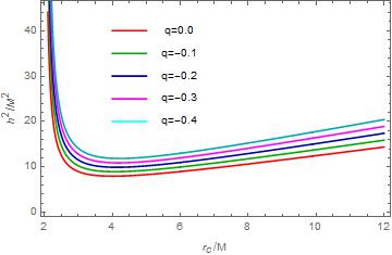
The effect of the probe charge, especially whether it is of same or opposite sign as the black hole charge, is quite striking. Intuitively we can argue that for the opposite sign case the probe charge effect will not be very significant because both the gravitational force and Coulomb force will be attractive and so qualitatively similar behavior to the neutral case will be observed. This is shown in Figure 1.

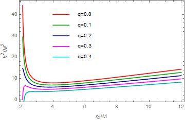
On the other hand, if the probe and black hole charges are of same sign the Coulomb force will be repulsive whereas the gravitational force is attractive as before. Interplay between these two forces produces an upper bound of the $q$ parameter above which the results become unphysical. This is demonstrated in Figure 2.

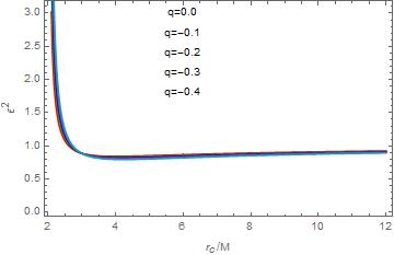
Similar behavior for $\epsilon^{2}=(E/m)^{2}$ vs. $r_{c}/M$ is observed in Figure 3 and in Figure 4 where, negative and positive values of $q$ are considered respectively.

The minimum radius for a stable circular orbit will occur at the point of inflection of the function $f(u)$, i.e.,

$\displaystyle f^{\prime\prime}(u)=-12Q^{2}u^{2}+12Mu-2(1+\frac{Q^{2}}{h^{2}}-\frac{Q^{2}q^{2}}{h^{2}})$

(63)

Eliminating $h^{2}$ from the above equation using (59) , we can write,

$\displaystyle 4Q^{4}u_{c}^{3}-9MQ^{2}u_{c}^{2}+6M^{2}u_{c}-M-qQ\left[qQ(4u_{c}^{3}Q^{2}-3Mu_{c}^{2})-\frac{E}{m}(6Q^{2}u_{c}^{2}-6Mu_{c}+1)\right]=0,$

(64)

or, in terms of $r_{c}$ ,

$\displaystyle r_{c}^{3}-6Mr_{c}^{2}+9Q^{2}r_{c}-\frac{4Q^{4}}{M}-\frac{qQE}{m}(\frac{r_{c}^{3}}{M}-6r_{c}^{2}+\frac{6r_{c}Q^{2}}{M})-q^{2}Q^{2}(3r_{c}-\frac{4Q^{2}}{M})=0.$

(65)

Let us define a parameter $\Lambda=(qQE)/(mM)$, in terms of which the above equation is rewritten as

$\displaystyle r_{c}^{3}(1-\Lambda)-6Mr_{c}^{2}(1-\Lambda)+9Q^{2}r_{c}(1-\frac{2}{3}\Lambda-\frac{q^{2}}{3})-\frac{4Q^{4}}{M}(1-q^{2})=0.$

(66)

Ignoring $O(Q^{4})$ terms we obtain

$\displaystyle r_{c}=3M\pm 3M{\sqrt{1-\frac{Q^{2}(1-\frac{2}{3}\Lambda-\frac{q^{2}}{3})}{M^{2}(1-\Lambda)}}}.$

(67)

Note that for $q=0$ that is neutral probe the earlier result (48)

$$r_{c}=6M-\frac{3Q^{2}}{2M}+...$$

is recovered. Considering $q$ and $\Lambda$ to be small (which is quite natural) we find

$\displaystyle r_{c}=6M-\frac{3Q^{2}}{2M}(1+\frac{\Lambda}{3}).$

(68)

This shows that the effective charge of the black hole increases for positive $\Lambda$ that is when the probe charge $q$ and black hole charge $Q$ are of same sign but it decreases when they are of opposite sign. This concludes our discussion on charged particle trajectory in the presence of a charged black hole.

Study of the Gaussian curvature for the Jacobi metric for Reissner- Nordstrom black hole, as experienced by a particle of fixed energy $E$ is the other major contribution of our work. The Jacobi metric corresponding to Reissner- Nordstrom geometry (20) (considering the system in the equatorial plane $\theta=\frac{\pi}{2}$)

$$ds^{2}=(E^{2}-m^{2}+\frac{2Mm^{2}}{r}-\frac{Q^{2}m^{2}}{r^{2}})[\frac{dr^{2}}{(1-\frac{2M}{r}+\frac{Q^{2}}{r^{2}})^{2}}+\frac{r^{2}d\phi^{2}}{(1-\frac{2M}{r}+\frac{Q^{2}}{r^{2}})}]$$

vanishes when

$\displaystyle E^{2}=m^{2}(1-\frac{2M}{r}+\frac{Q^{2}}{r^{2}}).$

(69)

The equation saturates for a critical value $r_{c}$:

$\displaystyle r_{c}=\frac{Mm^{2}\left(1+(1-\frac{(m^{2}-E^{2})Q^{2}}{M^{2}m^{2}})^{\frac{1}{2}}\right)}{m^{2}-E^{2}}\approx 2M(\frac{m^{2}}{m^{2}-E^{2}}-\frac{Q^{2}}{4M^{2}})+~O(Q^{4}).$

(70)

This leads to an inequality of the form $\frac{m^{2}}{m^{2}-E^{2}}\geq\frac{Q^{2}}{4M^{2}}$ and since $\frac{m^{2}}{m^{2}-E^{2}}<1$, one has $Q<2M$. It is interesting to recall that $Q=M$ is the extremality condition and moreover $Q<M$ is generally assumed to avoid the presence of a naked singularity (or violation of Cosmic Sensorship hypothesis by Penrose). Hence $Q<2M$ derived above is a weaker condition and does not add any further restrictions on the charge mass ratio.

Interpreting the following expression as Jacobi circumference [5]

$\displaystyle 2\pi(E^{2}-m^{2}+\frac{2Mm^{2}}{r}-\frac{Q^{2}m^{2}}{r^{2}})^{\frac{1}{2}}\frac{r}{(1-\frac{2M}{r}+\frac{Q^{2}}{r^{2}})^{\frac{1}{2}}}$

(71)

the boundary $r_{c}$ actually reduces to a point since the circumference vanishes there.

Condition for circular geodesics is derived from the extrema of the Jacobi circumference,

$\displaystyle\frac{E^{2}}{m^{2}}=\frac{(1-\frac{2M}{r}+\frac{Q^{2}}{r^{2}})^{2}}{(1-\frac{3M}{r}+\frac{2Q^{2}}{r^{2}})}.$

(72)

Circular orbits exist provided $(1-\frac{3M}{r}+\frac{2Q^{2}}{r^{2}})\geq 0$. This means that to $O(Q^{2}/M)$ the roots are

$$r_{+}=3M-(2Q^{2})/(3M),~r_{-}=(2Q^{2})/(3M)$$

indicating that $r\geq 3M-(2Q^{2})/(3M)$.

Several examples of radii (to $O(Q^{2})$) for some specific values of energy are provided below: for $m^{2}=0$, the term $(1-\frac{3M}{r}+\frac{2Q^{2}}{r^{2}})$ must be equal to zero leading to $r\approx 3M-\frac{2Q^{2}}{3M}$. The outermost and innermost circular orbit radii are computed by extremizing r.h.s of (72). These are respectively $r\approx 6M-\frac{3Q^{2}}{2M}$ for $E^{2}\approx m^{2}\left[\frac{8}{9}-\frac{2Q^{2}}{81M^{2}}\right]$ and $r\approx 4M-\frac{Q^{2}}{M}$ for $E^{2}=m^{2}$. Incidentally the last example agrees with our previously derived result (48). For $Q=0$ the above reduce to the Schwarschild geometry results [5].

Let us now come to the explicit structure of Gaussian curvature $K$. As a warmup exercise let us compute $K_{S}$ for Schwarschild case. Expressing the Jacobi metric pertaining to Schwarschild geometry as,

$\displaystyle ds^{2}=f(r)^{2}[dr^{2}+r^{2}(1-\frac{2M}{r})d\phi^{2}]$

(73)

where,

$$f(r)^{2}=(E^{2}-m^{2}+\frac{2Mm^{2}}{r})\frac{1}{(1-\frac{2M}{r})^{2}}$$

the Gaussian curvature $K_{S}$ is given by,

	$\displaystyle K_{S}$	$\displaystyle=$	$\displaystyle-\frac{1}{f(r)^{2}r(1-\frac{2M}{r})^{\frac{1}{2}}}\frac{d}{dr}\left[\frac{1}{f(r)}\frac{d}{dr}\left(rf(r)(1-\frac{2M}{r})^{\frac{1}{2}}\right)\right]$		(74)
		$\displaystyle=$	$\displaystyle\frac{M[m^{4}(2M-r)^{3}+E^{4}r^{2}(3M-2r)+3E^{2}m^{2}r(2M-r)(M-r)]}{r^{3}[m^{2}(2M-r)+E^{2}r]^{3}}.$		(75)

For massless probe $m=0$, the curvature simplifies to,

$\displaystyle K_{S}=-\frac{2M}{E^{2}r^{3}}(1-\frac{3M}{2r}).$

(76)

For $r\geq 2M$, $K_{S}$ is always negative [10].

References

- [1] D. Pugliese, H. Quevedo, R. Ruffini, Eur. Phys. J. C (2017) 77: 206 (arXiv:1304.2940).
- [2] D. Pugliese, H. Quevedo, R. Ruffini, Phys. Rev. D 88, 024042 (2013) (arXiv:1303.6250).
- [3] D. Pugliese, H. Quevedo, R. Ruffini, Phys.Rev.D84:044030,2011 (arXiv:1105.2959); Eur.Phys.J.C71:1638,2011; Phys.Rev.D83:104052,2011; Phys.Rev.D83,024021, 2011, (arXiv:1012.5411).
- [4] S. Grunau and V. Kagramanova, Phys. Rev. D 83 (2011) 044009 [arXiv:1011.5399 [gr-qc]].
- [5] G W Gibbons 2016 Class. Quantum Grav. 33 025004 (arXiv:1508.06755).
- [6] S. Chanda, G.W. Gibbons, P. Guha, J. Math. Phys. 58 (2017) 032503 (arXiv:1612.00375); Int. J. Geom. Methods Mod. Phys. 14, 1730002 (2017) (arXiv:1612.07395).
- [7] M Szydlowski, M. Heller and W. Sasin, J. Math. Phys. 37 346 (1996).
- [8] A. V. Tsiganov, The Maupertuis principle and canonical transformations of the extended phase space, J. Non-lin Math. Phys. 8 (2001) 157-182, arXiv: nlin/0101061.
- [9] O. C. Pin, Curvature and Mechanics, Advances in Mathematics 15 (1975) 269-311.
- [10] G. W. Gibbons and M. C. Werner, Class. Quant. Grav. 25 (2008) 235009 [arXiv:0807.0854 [gr-qc]]; G. W. Gibbons and C. M. Warnick, Phys. Rev. D 79 (2009) 064031 [arXiv:0809.1571 [gr-qc]].
- [11] G. W. Gibbons, C. A. R. Herdeiro, C. M. Warnick and M. C. Werner, Phys. Rev. D 79 (2009) 044022 [arXiv:0811.2877 [gr-qc]]; M. C. Werner, Gravitational lensing in the Kerr-Randers optical geometry, Gen. Rel. Grav. 44 (2012) 3047.
- [12] A. Deriglazov, Classical Mechanics, Hamiltonian and Lagrangian Formalism; DOI 10.1007/978-3-642-14037-2, Springer Heidelberg Dordrecht London New York.
- [13] S. Chandrasekhar, The Mathematical Introduction of Black Holes (Oxford University Press, New York, 1983).
- [14] M. Olivares, J. Saavedra, C. Leiva, and J. R. Villanueva, Mod. Phys. Lett. A 26, 2923 (2011) (arXiv:1101.0748).
- [15] Sir G. Greenhill, “Newton-Einstein planetary orbit,” Phil. Mag. (6) 41 (1921) 143-141
7 Appendix A
Explicit solutions for the constants given in [5] for Schwarzschild background are,