Stability of the phase motion in race-track microtons Note: Research supported in part by MINECO-FEDER grant MTM2015-65715-P(Spain) and CUR-DIUE grants 2014SGR504 and 2014SGR846 (Catalonia). T. M. Seara is also supported by the Russian Scientific Foundation grant 14-41-00044 and the European Marie Curie Action FP7-PEOPLE-2012-IRSES: BREUDS. We acknowledge the use of the UPC Applied Math cluster system for research computing. Useful conversations with Amadeu Delshams, Vasiliy Shvedunov, and Arturo Vieiro are gratefully acknowledged.
Abstract
We model the phase oscillations of electrons in race-track microtrons by means of an area preserving map with a fixed point at the origin, which represents the synchronous trajectory of a reference particle in the beam. We study the nonlinear stability of the origin in terms of the synchronous phase —the phase of the synchronous particle at the injection. We estimate the size and shape of the stability domain around the origin, whose main connected component is enclosed by the last rotational invariant curve. We describe the evolution of the stability domain as the synchronous phase varies. Besides, we approximate some rotational invariant curves by level sets of certain Hamiltonians. Finally, we clarify the role of the stable and unstable invariant curves of some hyperbolic (fixed or periodic) points.
Keywords:
Stability domain , invariant curve , Hamiltonian approximation , exponentially small phenomena , microtron1 Introduction
Race-track microtron (RTM) is a specific type of electron accelerator with beam recirculation combining properties of the linear accelerator and a circular machine [14, 34]. For applications in which a modest beam power at a relatively high beam energy is required the RTM turns out to be the most optimal source of electron beams. This is the case of applications like the cargo inspection or Intraoperative Radiation Therapy for which RTMs allow to get pulsed and continuous beams in a quite cost and energy effective way with the most optimal dimensions of the machine. An example of such accelerator is a compact 12 MeV RTM which is under construction at the Technical University of Catalonia in collaboration with the Moscow State University and CIEMAT (Spain) [1, 18, 48].
In the design of a particle accelerator its main parameters are optimized for some reference particle, usually referred to as synchronous particle. Real particles of the beam perform transverse and longitudinal oscillations with respect to this synchronous particle. One of the important issues of the RTM design is to assure the stability of these oscillations, in particular to avoid an uncontrolled growth of their amplitude that leads to the loss of the beam. In the RTM beam dynamics the main role is played by longitudinal oscillations of individual electrons with respect to the synchronous particle [46, 22]. Such oscillations are usually referred to as phase motion, and the region of initial states in the phase space which give rise to stable oscillations is called acceptance.
Stability of the phase oscillations of particles in the beam is a matter of primary concern both at the stage of the accelerator design and during its operation. In particular, the size of the acceptance determines the efficiency of caption into acceleration of particles injected from a source of electrons, usually an electron gun. The shape and size of the acceptance depend on the phase of the synchronous particle, also called synchronous phase and denoted as along this paper. The definition of these notions will be given in Section 2. A specific feature of the RTM is that the range of values of for which the acceptance exists is quite narrow and therefore this parameter must be carefully chosen and controlled during the RTM operation. The main criteria here is to keep the synchronous phase equal or close to the value for which the size of the acceptance is maximal and to avoid resonant values of . The latter is important because resonant phase oscillations lead to a buildup of beam instabilities, rapid growth of the amplitude of the phase oscillations and eventually to a loss of the beam. Therefore, a good understanding of the longitudinal dynamics of the beam in RTMs in general and the phase oscillations of electrons in a particular machine is important.
The phase oscillations of the beam in an RTM are described by a system of nonlinear difference equations [10, 34] that will be derived in Section 2. It gives rise to an analytic area preserving map which is the object of study in the present paper. These difference equations cannot be approximated by differential equations without loss of accuracy, since RTMs have large energy gain per turn and high frequency of phase oscillations. The description of the acceptance in the linear approximation is well known [34]. The change of the acceptance under the variation of the synchronous phase, the appearance of stable regions, and the emergence of the stochastic regime is studied in [26] by looking at the normal form of the difference equations up to order four. For instance, it was shown that there is a shift of the center of oscillations and that the oscillation frequency depends on the amplitude. We will reproduce these known results at the beginning of our analysis.
In the present paper we will study the phase motion of the beam in RTMs using modern Dynamical Systems methods. Our goal is to characterize the acceptance, called stability domain in Dynamical Systems, as a function of the synchronous phase. In particular, we will establish the intervals of values of for which the acceptance and its central connected component exist, analyze their geometry, shape and size, and calculate their area for the whole range of . Our main theoretical tools are the Moser twist theorem and several Simó’s stability results [39]. We will also approximate some rotational invariant curves of the RTM beam longitudinal dynamics by level curves of suitable Hamiltonians. Finally, we will carry out a global study of the acceptance and its connected component using results and algorithms, like the orbit method, developed in [23, 47].
The article is organized as follows. We give a short introduction into the RTM beam longitudinal dynamics, define the notion of synchronous trajectory and synchronous phase and derive the map describing the longitudinal beam dynamics that we will refer to as RTM map in Section 2. We introduce the notion of the acceptance and its connected component, we find fixed points of the RTM map and analyze their type in the linear approximation in Section 3. We also formulate a theorem about the local stability of the synchronous trajectory and give a summary of further results on the behavior of the acceptance as a function of the synchronous phase. The proof of the theorem is given in Section 4. Section 5 is devoted to the approximation of the RTM map by the integrable dynamics of certain Hamiltonians and correspondingly the approximation of the invariant curves around the synchronous trajectory by means of Hamiltonian level curves. The global stability of the synchronous trajectory is studied in Section 6, also a detailed characterization of the acceptance is given there. These results are obtained numerically by using the orbit method. The invariant curves of hyperbolic points are analyzed in Section 7. A summary and a discussion of the obtained results are given in Section 8.
2 The RTM model
The operation of a race-track microtron (RTM) is illustrated in Fig. 1. The initial beam is injected from an electron source (electron gun or external pre-accelerator) into an accelerating structure (AS) consisting of a few resonant cavities. The longitudinal electric component of a high frequency electromagnetic wave (usually a standing wave) accelerates the electrons in the AS. Then the beam is bent by the magnetic field of a bending magnet, called end magnet, travels through a free space, usually referred to as drift space, follows along a circular trajectory inside the second end magnet and returns to the AS. In this way the beam makes a number of recirculations through the RTM with the energy being increased at each pass through the AS. Once the beam gets the final design energy, it is deflected by an extraction magnet and is directed towards the accelerator beam exit.
We approximate the AS by a zero length accelerating gap and consider a stationary regime with a constant amplitude of the accelerating field. Then the energy gain of an electron passing through the AS is equal to , where is the maximum energy gain in the AS and is the phase of the accelerating field. In accelerator physics this parameter is usually referred to as particle phase and is used to characterize the longitudinal position of the particle along the orbit with respect to the accelerating gap (in a real machine with respect to, say, the exit, of the last cavity of the AS in the direction of the beam motion). Another idealization in our study is that the end magnets will be considered as hard-edge dipole magnets so that the fringe-field effects are not taken into account.
Let us consider the longitudinal (phase) motion of electrons in an RTM with magnetic field induction in the end magnets and separation between the magnets (straight section length). We assume that the injected electrons are already ultra-relativistic, so that in the formulas below the velocity of the particles in the beam is equal to the velocity of light .
Our dynamical variables are the full particle energy and its phase at the -th turn at some point of the orbit. For the sake of convenience, we choose this point to be the exit of the AS. Let and be the particle phase and energy at the injection; that is, just before its first passage through the AS. We would like to note that, in some pulsed RTM, the electrons reverse their trajectory in special reverse field magnets after the injection and first acceleration at the AS [18, 48]. In that case, is the energy after the first acceleration and reflection of the beam in the end magnet, before the second passage through the AS, but we will still use the term injection energy.

For the RTM model described above, the duration of the -th revolution of the beam is
| (1) |
where is the elementary charge and is the beam trajectory radius in the end magnets. We have used that in bending magnets for ultrarelativistic beams [34]. Relation (1) allows us to work indistinctly with time variables or energy variables . The beam dynamics in the phase-energy variables, for a zero-length AS, is governed by the difference equations
| (2) |
being the period of the accelerating electromagnetic field, usually called radiofrequency (RF) field in the context of accelerator beam dynamics. See [34].
The design of a particle accelerator requires a proper choice of physical and technical parameters in order to guarantee the existence of a reference trajectory, called synchronous trajectory, so that an ideal particle following this trajectory is accelerated in the most optimal way. Namely, it can be tuned in resonance with the accelerating field. Let us explain the choice of parameters in case of an RTM. We fix two positive integers and . The resonance conditions in the case of an RTM are
| (3) |
Henceforth, the subindex “” indicates quantities related to the synchronous trajectory. The integer is the number of RF field periods during the first turn and defines the synchronicity condition at this turn, whereas is the increase of the multiplicity factor due to the increase of the period of revolution of the reference particle in each turn. The ratio
is called harmonic number. RTMs are accelerators with variable harmonic numbers, since depends on the -th turn.
If we rewrite the resonance conditions (3) using the energy variables and relation (1), we get that , where
and is the wavelength of the RF field. Finally, it is straightforward to check that if the injection phase for the synchronous trajectory satisfies relation
then we get a particular solution of equations (1)–(2), whose energy undergoes a constant gain at each turn:
| (4) |
with . We note that , so this synchronous particle passes through the AS in the same phase of the RF field at each turn: (mod ) for all . We say that is the synchronous phase.
Once we realize that the synchronous trajectory (4) exists, we wonder whether the oscillations of other trajectories around it are stable. This depends on the synchronous phase .
We study this dependence by introducing the variables
| (5) |
that describe the phase and energy deviation of an arbitrary trajectory from the synchronous one. Then the beam dynamics is modeled by the map , where
For simplicity, we will assume that in the rest of the paper. The study of other values can be carried out in a similar way.
We end this section by stressing that the model of longitudinal oscillations around the synchronous trajectory for non-ultra-relativistic beams is more complicated [17].
3 Terminology and main results
Under the assumption , our model for the nonlinear oscillations around the synchronous trajectory (4) is the analytic area preserving diffeomorphism , defined by
| (6) |
Here, is a parameter, and (respectively, ) is the deviation of the phase (respectively, energy) of an arbitrary particle from the phase (respectively, energy) of the synchronous trajectory, which corresponds to the fixed point
The angular coordinate is defined modulo , so our phase space is , with . For brevity, we will write and . We look for initial conditions that give rise to particles with a bounded energy deviation from the synchronous trajectory. More precisely, we will estimate the size and the shape of
This domain is called (longitudinal) acceptance in Accelerator Physics, and stability domain in Dynamical Systems. We will also study its connected component that contains .
Remark 1
We have numerically checked that
Hence, if is the phase-energy deviation at the -th turn of a trajectory contained in and denotes the lift of this trajectory determined by , then for all . This means that trajectories with bounded energy deviation, have also bounded phase deviation respect to the synchronous one.
The map , its acceptance , and the connected component depend on , but we will frequently omit this dependence. Otherwise, we will write , , and , respectively.
We say that the synchronous trajectory is:
- 1.
Globally stable when is a neighborhood of ;
- 2.
Locally stable when there exists such that
- 3.
Linearly stable when the sequence is bounded, where is the linear part of the map at ; that is, when the linearized map is locally stable.
Otherwise, it is globally, locally, or linearly unstable.
Local stability implies global stability, but local instability does not imply global instability. The case is a sample of this claim. See Fig. 2(l). Our map (6) shows the four possible combinations of local stability/instability and linear stability/instability.
The synchronous trajectory is hyperbolic, parabolic, or elliptic when the eigenvalues of the matrix are real of modulus different from one, real of modulus equal to one, or non-real of modulus equal to one, respectively. We note that , since is an area preserving map. Therefore, the behavior in the linear approximation of the synchronous trajectory only depends on the trace . Concretely, it is hyperbolic, parabolic or elliptic if and only if , , or , respectively.
The linear type and the local stability are related as follows. The hyperbolic type implies local instability, whereas the elliptic type is generically locally stable, but local instability may take place in degenerate cases [37]. The parabolic type is the hardest one, but it can be studied using results from [21, 38, 39].
The linear part of the map (6) at the fixed point is
so . Thus, the linear type of depends on the parameter as follows. It is hyperbolic, parabolic or elliptic if and only if , , and , respectively.
If , then the eigenvalues of have the form
for some such that
| (7) |
This means that the linear dynamics around is conjugated to a rotation by angle .
If is an orbit of the map, then we say that it is unbounded when is unbounded in , and we say that it is homoclinic to the fixed point when , but . Any unbounded orbit is placed outside the acceptance.
The map (6) has two fixed points: and
The linear part of the map (6) at the fixed point is
so . Hence, is hyperbolic for any . Indeed, if , then the eigenvalues of have the form
for some such that
This means that the linear dynamics around expands the unstable direction by a factor and contracts the stable direction by a factor .
The quantity is called tune in Accelerator Physics [34]. Nevertheless, following a standard terminology in Dynamical Systems, we will say that is the rotation number of the elliptic fixed point . The elliptic point is called -resonant when for some relatively prime integers and such that , which implies that . Besides, is the order of the resonance. The quantity is the characteristic exponent of the hyperbolic fixed point .
The quantities and carry the main local information around the fixed points when .
Moser twist theorem is the standard tool to prove that fixed points of analytic area preserving maps are locally stable [37]. If the dynamics around the fixed point satisfies some twist condition, Moser twist theorem implies that any neighborhood of the fixed point contains infinitely many closed invariant curves. We say that such curves are rotational invariant curves (RICs) since they surround the fixed point and their internal dynamics is conjugated to a rigid rotation. The local stability follows from the fact that the domain enclosed by any RIC is invariant.
We will prove the following characterization in Section 4.
Theorem 1
The synchronous trajectory is locally stable if and only if .
The range of local stability in terms of and is given in Table 1.
| Relation | Local stability |
|---|---|
Once we have a clear understanding of the local dynamics, we focus on the global picture, which rises several questions. Which is the “last” RIC (LRIC)? How can we compute it? Does it coincide with the border of the connected component ?
If the border is an analytic curve and its internal dynamics is conjugated to a rigid rotation, then is the LRIC that we are looking for and we can numerically compute it by using the algorithm described in [41]. These two hypotheses about are not so restrictive as they may look. Indeed, all RICs obtained from the Moser’s twist theorem satisfy them. This means that even when does not satisfy them, probably there are many Moser-like RICs close to , which are the objects that our computations will find.
A summary of the phenomena that take place when moves is displayed in Fig. 2. If there exist RICs around the origin, we plot some of them, the last one (the LRIC), and one unbounded orbit very close to the LRIC. If the origin is globally unstable, we plot suitable unbounded orbits to highlight it. The invariant curves (ICs) displayed in Fig. 2(a) are no RICs for the synchronous trajectory, since they do not surround the origin.
Fig. 2 shows the basic skeleton from which an expert reader can deduce the main dynamical changes. Let us describe them.
The elliptic fixed point and the hyperbolic fixed point merge in a parabolic point as ; see Figs. 2(a)–2(c). This scenario corresponds to a saddle-center bifurcation [2, 6]. The stable and unstable invariant curves (called separatrices) of the hyperbolic fixed point seem to form a small loop around the elliptic fixed point when . The LRIC around the elliptic point is exponentially close (in the parameter ) to the separatrices. See Fig. 2(c). We will use this fact to see that
| (8) |
Therefore, both regions are almost the same when . (If is a subset of , then denotes its area.)
The LRIC grows in size, changes its shape, and moves away from the separatrices as increases; see Fig. 2(d). We reach the fourth order resonance at . The elliptic point is locally stable at this resonance, and the RICs near it look like a Latin cross, whose arms have a width of the order of the square of its length; see Fig. 2(e). The Hénon map displays exactly the same behavior at the fourth order resonance [38].
The twist coefficient (also called first Birkhoff coefficient) goes from negative to positive at and from positive to negative at , where the third order resonance takes place. This is one of the two typical behaviors for the twist coefficient described in [30]. It means that the orbits around the origin rotate slower (resp., faster) as they go away from the origin when (resp., ). Figs. 2(g)–2(i) show that behavior, since we see a three-periodic orbit near the elliptic point for both and .
The elliptic point is locally and globally unstable at the third order resonance; see Fig. 2(h). If with , the LRIC is approximately a triangle of vertices
| (9) |
In particular,
| (10) |
The LRIC grows in size and its triangular shape changes to a “banana-like” shape as the parameter moves from the three order resonance at to the second order resonance at . The fixed point is locally stable at this last resonance, and the RICs near it looks like “bananas” whose width is of the order of the square of its length. See Fig. 2(k).
Finally, a period-doubling bifurcation takes place after the second order resonance. To be precise, the point becomes a saddle for , being parabolic with reflection at . One then expects to find an elliptic two-periodic orbit for . The separatrices of the hyperbolic fixed point form two small loops around the two elliptic two-periodic points. Nevertheless, the saddle remains globally stable when , since some of the RICs around still persist. See Fig. 2(l).
In spite of all the above comments, the expulsion of some resonance is a more relevant phenomenon than any resonance at the elliptic fixed point, but the third order resonance. The reason is that only the first phenomenon changes drastically and , since the second one takes place inside . We will check that and experiment a jump for each primary resonance that is thrown away. Besides, these primary jumps are smaller in than in . However, displays many more jumps, the secondary ones, which are related to resonances inside elliptic islands that are already outside . We will visualize such properties in Section 6.
4 Local stability of the synchronous trajectory
This section has a purely local character. It contains the proof of Theorem 1. The hyperbolic type always implies local instability, so we only study the range .
4.1 Local instability in the saddle-center bifurcation
4.2 Local stability in the elliptic case: Generic values
Let . Then the point is elliptic with rotation number . The relation between and is given in Table 1.
First, we bring the linear part of map (6) around the elliptic fixed point into its real Jordan normal form
by means of an area preserving linear change . We write our map in these new variables as
Then we introduce the complex variables and . The map reads in these variables as
| (11) |
for some complex coefficients , which depend on the original parameter . We recall that .
If for some integer such that , then we say that the elliptic point is strongly resonant. It is known [37] that if the elliptic point is not strongly resonant, then there exists an area preserving polynomial change of variables which brings the map (11) into its third order Birkhoff normal form
| (12) |
for some real coefficient , called first Birkhoff coefficient or twist coefficient. It turns out that
where denotes the imaginary part of , see [30, 13]. The coefficients and also depend on , via the parameter . After some tedious computations [20], one gets the expression
| (13) |
We observe that , , and exist and are negative. That is, has a negative fourth-order pole at , a negative simple pole at , and a negative second-order pole at . These properties agree with the generic behavior of twist coefficients of families of area-preserving maps described in [30].
Consequently, we deduce that has at least one root in the interval . Let us prove that it has no more real roots. The numerator in (13) is the polynomial in the variable , with , , , and . This cubic polynomial has one real root and two complex conjugated roots, because its discriminant is negative:
This means that has just one root in the interval . It was numerically computed in [20] that
We have plotted the twist coefficient versus in Fig. 3.
4.3 Local stability in the fourth order resonance
We consider the area preserving linear change of variables
| (14) |
This change brings the linear part of the map at the origin into its real Jordan normal form . Indeed, the map becomes
| (15) |
Let be the Taylor expansion of . We know from Corollary 4.2 in [39] that if and , then the origin is locally unstable under the analytic map (15) if and only if
In our concrete map, and . Therefore, the synchronous trajectory is locally stable when , and we will analytically study the shape of its RICs in Section 5.2.
4.4 Local stability for the root of the twist coefficient
If , then the third order Birkhoff normal form (12) does not provide much information because the first Birkhoff coefficient vanishes. Thus, we should compute the fifth order Birkhoff normal form
where and is the second Birkhoff coefficient. The analytical computation of is cumbersome, so we have taken a simpler numerical approach. First, we have computed the rotation number of the points of the form using the algorithm described in subsection 6.2. Next, we have checked that
| (16) |
for some non-zero coefficient , which implies that . Then the Moser twist theorem implies that the origin is a stable elliptic fixed point [37].
4.5 Local instability in the third order resonance
Set . Then the map (6) takes the form
The map is close to the identity, since
We determine the local stability of the origin under the map (and so, under the map ) by applying Simó’s criterion [39]. That criterion states that the origin is locally stable under an analytic area preserving map of the form
if and only if has a strict extremum at the origin, where is the generating function of the map; that is, is a function determined by the implicit equations
| (17) |
Thus, we look for a function such that
After a straightforward computation, we obtain that
This function has no strict extremum at the origin. Therefore, the synchronous trajectory is unstable when . We will give more details about the dynamics around the origin near this third order resonance in Section 5.3.
4.6 Local stability in the second-order resonance
We consider the area preserving linear change of variables
which brings the linear part of the map at the origin into its Jordan normal form. Indeed, the map becomes
| (18) |
Let be the Taylor expansion of . We know from Lemma 1.4 in [39] that if , , and , then the origin is locally stable under the analytic map (18).
In our concrete map, and . Therefore, the synchronous trajectory is locally stable when .
This completes the proof of Theorem 1.
5 Hamiltonian approximations
This section contains a semi-local study of the RICs around the synchronous trajectory. We will approximate them by the level curves of suitable Hamiltonians in three different scenarios. We will also prove the asymptotic formulas (8) and (10).
5.1 Near the saddle-center bifurcation
Let us study the size and shape of when .
The elliptic fixed point and the hyperbolic fixed point of the map (6) collapse as . The following rough quantitative estimates are typical for saddle-center bifurcations. The size of in the -coordinate is . Its size in the -coordinate is , since the angle between the eigenvectors of the matrix is . Consequently, . Finally, when . We will confirm and refine these rough estimates.
Following the above comments, we scale the -coordinate (respectively, -coordinate) by a factor of order (respectively, order ). To be precise, we consider the change of scales
| (19) |
If , then the map (6) is transformed under this change into a map of the form
| (20) |
The map is close to the identity map , since
The area-preserving character of implies that the term is a Hamiltonian vector field. Concretely,
where the Hamiltonian is given by
| (21) |
We have subtracted the constant for convenience. We denote by the -time flow of a Hamiltonian . Then
| (22) |
since the Euler method has a second order local truncation error.
Therefore, the integrable dynamics of the Hamiltonian approximates the dynamics of the map in the limit . We say that is the limit Hamiltonian associated to the saddle-center bifurcation. It has two equilibrium points. Namely, the elliptic point and the saddle point . Besides, the unstable and stable invariant curves of the saddle point coincide along one branch, giving rise to the separatrix
Let be the domain enclosed by ; that is,
The phase portrait of the limit Hamiltonian (21) is sketched in Fig. 5. Only the points inside the domain give rise to bounded trajectories. This implies that is a good approximation of the scaled versions of and when .
The separatrix is described by a homoclinic trajectory to the saddle point: . If we impose the initial condition and solve the Hamiltonian equations on the separatrix , we get that
| (23) |
Therefore,
The first identity follows from Green’s theorem, the last one follows from the residue’s theorem. The asymptotic estimate (8) follows from the change of scales (19).
Fig. 6 shows a strong agreement between the numerically computed values of and and their asymptotic estimate , even for relatively big values of .
Next, we compute better Hamiltonian approximations near the saddle-center bifurcation. The Lie’s series method is the standard tool to find them, however we will follow a generating function method that fits perfectly with the map (20).
We recall the following formal result from [39, Remark 1].
Let be an analytic area preserving map that is, in some sense, close to the identity. Let be a function such that is a generating function of ; that is, it satisfies the implicit equations (17). We note that . The 1-time flow of the Hamiltonian defined by
and so on, coincides with the map at a formal level. There is a small misprint in [39]; the numerical factors in the fourth term are , not . Besides, we must skip the minus signs in front of the even terms that appear in [39], because our generating function has the form , instead of . Here, subindexes in mean partial derivatives. We note that . The series is generically divergent. Otherwise, would be integrable, which is an exceptional situation.
Now, we come back to our concrete problem.
We write the map (20) as
where
Then it is easy to check that the function
satisfies the implicit equations (17), where is the limit Hamiltonian (21). Let be the formal series associated to this generating function. We note that , and so for all . Therefore, if we retain just the first terms of the formal series, we get an approximating Hamiltonian such that
It is interesting to compare this formula with (22). On the other hand, using the stronger estimate , we get that for some function that does not depend on for all . Indeed,
since all mixed partial derivatives of vanish.
We have plotted some level curves of the approximating Hamiltonian
for in Fig. 7. We have used the original coordinates for the sake of comparison, instead of the scaled ones (19). We have also plotted some RICs of the microtron map (6). We stress that, in spite of the relatively big value of , the RICs fit surprisingly well with the level curves, being this fitting better close to the elliptic fixed point. The fitting improves when is smaller. The LRIC is represented in a thick line. The “last” level curve correspond to the value .
Finally, let us discuss briefly how to refine the asymptotic estimate , although we do not carry out the associated computations. They are too cumbersome.
If , the Hamiltonian has, besides the elliptic point , a hyperbolic saddle point close to whose unstable and stable invariant curves coincide along one branch. Let be the domain enclosed by the corresponding separatrix. Then for some coefficients . We have already seen that . In this way, we may get the refined asymptotic estimates
Anyway, we stress that is not smooth in the parameter . Rather the opposite happens; has a fractal self-similar structure with infinitely many jumps, although they become very small when . See [41, 42], Fig. 6, and Fig. 13.
5.2 At the fourth order resonance
Let be the transformed map in the coordinates (14), which were the suitable ones for .
The map is very close to the identity in a neighborhood of the origin when . To be precise, . Hence, given any order , there exists a unique approximating Hamiltonian of the form
being a homogeneous polynomial of degree , such that
A rather tedious computation, which we have the good taste to omit, leads to the following formulas:
with , , .
All approximating Hamiltonians are symmetric:
This is a consequence of the fact that the reversor that we will give in (26) becomes in the coordinates (14).
We have plotted some level curves of the Hamiltonian
in Fig. 8. We have used the original coordinates . The RICs of the microtron map fit quite well with the level curves. Of course, the fitting improves close to the origin. The LRIC is represented in a thick line. The “last” level curve correspond to the value .
5.3 Near the third order resonance
Let us study the size and shape of the connected component of the acceptance when with . We will see that is approximately a triangle of vertices (9), which implies that the asymptotic estimate (10) holds. We scale the variables according to these claims, which suggest that all the interesting dynamics takes place in a -neighborhood of the origin. To be precise, we consider the change of scale
| (24) |
If with , then the map (6) is transformed under this change into a map of the form
The map is close to the identity: , with
Following Section 5.1, we realize that the first order term is a Hamiltonian vector field with Hamiltonian , where
| (25) | |||||
Therefore, , and the integrable dynamics of the Hamiltonian approximates the dynamics of the map when . Thus, is the limit Hamiltonian associated to the third order resonance. It has four equilibrium points. One elliptic point: , and three saddle points:
Let be the triangle whose vertices are these three points. Clearly, . Each side of is both the stable invariant curve of a saddle, and the unstable invariant curve of another saddle. That is, is formed by the three saddles and the three straight separatrices connecting them. See Fig. 9.
Only the points inside the closed domain give rise to bounded trajectories, so is a good approximation of the scaled version of for . Thus, we get the quadratic asymptotic estimate (10). We have displayed a comparison between the numerically computed area and its asymptotic estimate in Fig. 10. We note that , because of the traces of the -periodic chain of elliptic islands that was thrown away from the main connected component at some value . We will visualize these traces in Fig. 14.
6 Global stability of the synchronous trajectory
This section has a global and experimental character. We will numerically study the stability domain and its connected component in the range . We will also describe some ideas behind the algorithms.
6.1 The reversors
A map is reversible when each orbit is related to its time reverse orbit by a symmetry transformation, called a reversor. If a map is reversible, many of their periodic and homoclinic points are located on certain symmetry lines, and many of their invariant objects are invariant under the reversors [4]. Two paradigmatic examples of such invariant objects are RICs around elliptic points and stable and unstable invariant curves of hyperbolic points. We will use these facts to simplify some computations.
The map (6) can be written as the composition , where are the involutions
| (26) |
and . This means that the map is reversible with reversors and . See [19]. The symmetry lines of these reversors are their sets of fixed points; that is,
| (27) | |||||
All the RICs displayed in Fig. 2 are invariant under the reversors and , and so is the stability domain . See Fig. 11.
In particular, if we consider the decomposition
then . This halves the computational effort to find . The connected component satisfies the same property.
The symmetry lines of any reversible map have many more useful properties. Let us recall the characterization of symmetric periodic orbits (SPOs) given in [19]. SPOs are the periodic orbits that are invariant under both reversors and . An orbit of is an SPO if and only if it has exactly two points on , in which case it has a point on each symmetry line if and only if it has odd period. We have displayed in Fig. 11 a couple of -SPOs. Four is even, so one of these orbits has two points on , and the other orbit has two points on .
6.2 The rotation number
The points inside the stability domain rotate around the elliptic fixed point when . The points infinitesimally close to give turns per iteration, where is the angle defined in (7). We recall that is the rotation number of the elliptic point , and we write . Next, we try to define the rotation number for any point following a standard approach [15].
Given any , let be its “argument”. That is, is the angle between the segment and the semi-straight line . Analogously, let be the “argument” of the -th iterate . We consider these arguments on the universal cover , not on . Then we wonder whether the limit
| (28) |
exists. If so, we say that (28) is the rotation number of the point under the map around the elliptic point . We may be tempted to use the crude numerical approximation
for big enough values of , but it has an -error in the most common situations. Fortunately, it can be refined using the following algorithm. See [35, 23] for details.
Given two integers , we set and compute
for , , and . Then, under some mild hypotheses, the refined approximation
has an -error. Furthermore, we have the following empirical bound of the error in the analytic setting:
| (29) |
We are interested in rotation numbers because they allow us to distinguish the three main bounded dynamical behaviors in analytic area-preserving diffeomorphisms [15, 41, 35]:
- 1.
If is a Moser-like RIC, then the limit (28) exists for all , and it does not depend on , so we write . Besides, is, generically, a Diophantine number (that is, it is badly approximated by rational numbers), and the previous refined algorithm works quite well.
- 2.
A -periodic chain of elliptic islands is an invariant region with several connected components such that each of them surrounds a -periodic elliptic point. The -periodic chain around around is displayed in Fig. 11 for two values of . It is formed by the four big green domains. Each of them is mapped onto the next one in clockwise sense, so for any point inside them. Similarly, if is inside an -periodic chain of elliptic islands, the limit (28) exists, , and the refined algorithm also works quite well.
- 3.
From now on, we paint the points inside chaotic seas in blue, the ones inside elliptic islands in green, and the ones on RICs in red. Fig. 11 and Fig. 12 are samples of that convention. To be precise, given any point , we apply the refined algorithm with and to compute its rotation number. If the empirical bound (29) is bigger than the tolerance , then we paint in blue. Otherwise, we paint in red/green when is irrational/rational, which is decided by looking at its continued fraction; see [16] for details.
Finally, we can understand the meaning of the small gaps that appear in the graph of the function displayed in Fig. 4. They simply correspond to the sections of some chaotic seas with the symmetry line . The rotation number is not well defined on those sections.


6.3 The stability domain
We compute the stability domain of the microtron map (6) using the orbit method described in [47]. Visual examples of several stability domains of the Hénon map provided by this method can be found in [42, 43, 44]. Our figures show a strong resemblance with those ones.
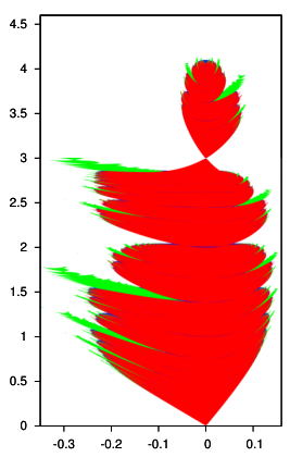
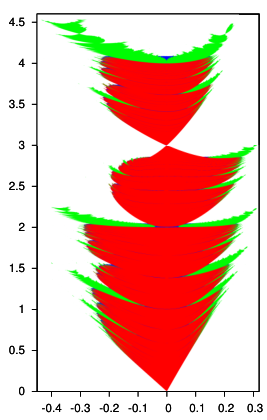
Let us describe our implementation of the orbit method.
First, we take a fine rectangular grid in a suitable rectangle
that contains the upper half of the stability domain. Second, we paint in white all grid points such that some of their first iterates escape from the control region
This is a fast step, since is a relatively small number for any modern computer. Third, we consider the -th iterates with of all not-yet-white grid points adjacent to some already-white one. If some of these iterates escapes from the control region, we paint in white all grid points “visited” by its corresponding unbounded orbit or by its -symmetric orbit. We do not use the reversor , since is computationally cheaper and . We repeat this process until no more points escape from the control region. This is the hardest step. Fourth, we determine the color of each non-white grid point by computing its rotation number as explained before. This step of the algorithm is not “orbitally coherent” in the sense of [47], but we feel that it is the right choice, since there is no clear way to choose the color in disputed cases. Finally, we get the lower half of the stability domain from the identity .
We stress that all grid points in the interior (respectively, “on” the border) of the stability domain have been iterated only 1000 (respectively, ) times. This is good, since the interior contains much more grid points than the border.
Fig. 11 shows a couple of stability domains computed with this algorithm. Each pixel is the center of a square with side , so the area of the stability domain is approximately equal to times the number of colored pixels. We also count the number of pixels in the connected component containing the origin following a standard algorithm in Computer Vision. See, for instance, [36, pags. 72–75]. In that way, we obtain that and for , but and for .
These jumps in and have a simple explanation. We recall that the fourth order resonance takes place at . After that value is crossed, four -periodic elliptic islands surrounded by a chaotic sea emanate from the elliptic point . This structure (elliptic islands plus chaotic sea) moves away from as grows, but remains inside while some RIC surrounds it. However, the LRIC surrounding it disappears at some value . After that value is crossed, both the elliptic islands and the chaotic sea are thrown away from the connected component , although any elliptic island is, by definition, part of . Thus, the jump in only takes into account the loss of the chaotic sea, whereas the jump in also takes into account the loss of many elliptic islands.
Similar jumps take place for any periodic elliptic island, although the greater is the order of the expelled island, the smaller is the jump in both areas. For instance, we see in Fig. 12 the stability domains for , , and , which are parameter values smaller than, but very close to, the values at which the periodic elliptic islands of orders three and five are thrown away from the connected component . Hence, the stability domains corresponding to , , and are significantly smaller, because the more extern chaotic sea is lost.
Fig. 13 shows and as a function of . The maximal value is attained for , for all , and for all . Obviously, , since . We note that displays many more jumps than , because it is affected by secondary resonances (resonances inside the islands). The graph of has a self-similar fractal structure caused by those secondary resonances, as the displayed magnification shows.
We also list in Table 2 the exact value
| (30) |
at which the elliptic fixed point becomes -resonant, so that the -periodic chain of elliptic islands is created from , jointly with the numerically approximated value at which the -periodic chain of elliptic islands is thrown away from , for all -resonances of order . For instance, the -periodic chain is thrown away at some value , which explains the seven “holes” delimited by the unbounded orbit displayed in Fig. 2(f) for .
We observe that , but in the -resonance, which comes as no surprise, since the twist coefficient is positive if and only if , see Subsection 4.2.
| Emanate at | Escape at with | |
|---|---|---|
We end with a couple of warnings regarding the accuracy of our pictures.
On the one hand, we know that the red domains displayed in Fig. 11, and in the left picture of Fig. 12 are not completely filled with RICs. Indeed, KAM theory implies that the set of all RICs has a complicated Cantorian structure, whose gaps are filled with resonances. Let us explain why we do not see those resonances. We restrict our explanation to the case of Fig. 11, since the phenomenon is the same in both cases. We do not see any resonance inside the red zone displayed in Fig. 11 because
when , see Table 1. Therefore, all missed resonances have orders , since is the rational number in the interval with the smallest denominator. Such resonances are too small to be detected with our pixel resolution. We recall that a generic -resonance in an -neighborhood of an elliptic fixed point of an analytic area preserving map has an -size [42].
On the other hand, the border of the connected component should be a red curve (the LRIC), which is missing in the left picture of Fig. 11 and in the three pictures of Fig. 12. The reason is, once more, that the LRIC is too thin to be detected with our pixel resolution. In the same way, probably there are some RICs in the middle of the blue zone, which would mean that that blue zone is composed by several chaotic seas, instead of by a single big chaotic sea.
6.4 The sections with the symmetry lines
We consider the sections of the stability domain with the symmetry lines (27) for two reasons. First, the stability domain is symmetric with respect to these lines. Second, we recall that each SPO has exactly two points on these lines, and such SPOs are the basic invariant objects that organize the dynamics inside their resonance.
We look at Fig. 11 to understand how SPOs organize the resonant dynamics. We see an elliptic -SPO with two points on that organizes the stable dynamics inside the four big green elliptic islands, and a hyperbolic -SPO with two points on whose stable and unstable invariant curves delimit almost perfectly the red region “filled” with RICs.
We do not deal with each one-dimensional section as a separate object, but we gather them into the two-dimensional sets:
in order to visualize their evolution in the parameter .
These sets are represented in Fig. 14 with the usual color codes. We see that the connected component collapses to the elliptic fixed point at , and undergoes its major loss at some . The collapse is associated to the local instability of the third order resonance. The loss takes place when the fourth order resonance is thrown away. These are the most relevant phenomena regarding the size of the stability domain in generic families of area-preserving maps.
We appreciate a clear self-similar fractal structure in the sets and . One can magnify their pictures to appreciate several details. Let us describe the main ones.
Resonances emanate from the elliptic fixed point in the form of thin blue and green tongues, since they are sections of chaotic seas surrounding elliptic islands. These tongues begin at the points , where is defined as in (30) for any rational number , so there are infinitely many of such tongues. Besides, they look symmetric with respect to the vertical line in a neighborhood of that line. The resonances, but the -one, have a small width when they are close to . Hence, most of the tongues become visible only at some distance of .
The elliptic islands inside a resonance grow in size when they move away from . If the resonance has even order, then the green part becomes the biggest part of the tongue in the set , but not in the set . This means that each elliptic SPO with even period has two points on , but none on . Fig. 11 is a sample of that empirical claim. On the contrary, if the resonance has odd order, then the green part becomes the biggest part of just one branch of the tongue, in both sets and . The other branch remains blue. This is a completely expected behavior, since we know that all SPOs with odd period have just one point on each symmetry line.
We warn that red and green regions should not be in direct contact, but we have again difficulties to detect the blue chaotic seas between them with our current pixel resolution.
Resonances are thrown away from , which is the reason for the saw-like border of and . Once a green tongue is separated from the main red body in the -direction, it is no longer delimited by blue portions, because chaotic seas do not form part of when their resonances are thrown away. See Fig. 11. Besides, the separated part of any green tongue shows a shape similar to the shape of the whole set, which is due to the secondary resonances. Indeed, we see the two above-mentioned phenomena (major loss in the stability domain and collapse of the stability domain to a point) along many of these tongues.
Such phenomena are clearly visible in the tongues of that cover the range . The fixed point is already globally unstable in that range, but there is still a locally stable elliptic two-periodic orbit on the symmetry line .
7 On the invariant curves of some hyperbolic points
The stable and unstable invariant curves of hyperbolic (fixed or periodic) points organize the dynamics of area preserving maps in several ways. Let us just mention two of them.
On the one hand, some of these invariant curves are approximate boundaries of stability domains [9], in which case the area of the lobes between them is equal to the flux through certain closed curves composed by arcs of invariant curves [28]. These lobes have an exponentially small area in the analytic case [5], so that the above-mentioned closed curves become partial barriers of the dynamics [24, 28]. If the map is entire, then the stable and unstable invariant curves never coincide [45], so these partial barriers are never complete barriers.

On the other hand, if the unstable invariant curve of some periodic orbit intersects the stable invariant curve of another periodic orbit, then there can be no RICs between both periodic orbits. This obstruction criterion was established in [32].
Next, we discuss these ideas in the setting of map (6).
7.1 Singular splitting near the saddle-center bifurcation
We saw in Section 5.1 that the map (6) is approximated, after the rescaling (19), by the -time flow of the Hamiltonian (21) when . Besides, the Hamiltonian (21) has a separatrix that encloses a region which resembles the stability domain of the map when . Compare the stability domain displayed in Fig. 2(c) with the phase portrait of the Hamiltonian (21) sketched in Fig. 5. The separatrix is described by the homoclinic trajectory (23), which is analytic in a complex strip of width .
Nevertheless, the stable and unstable invariant curves of the saddle point of our map (6) do not coincide, since the map is entire. This result goes back to Ushiki [45]. We have displayed the stability domain and the separatrices of the saddle point for in Fig. 15. We check that the separatrices enclose the stability domain. The reversibility of our map implies that the separatrices have a primary homoclinic point on each symmetry line (27). Let be the region (such region is called lobe) delimited by the pieces of the separatrices between these two primary homoclinic points. For instance, we display the lobe for in figure 16. In that case, the lobe area is .
Fontich and Simó [5] proved that the splitting of the separatrices for any close to the identity analytic area preserving map is exponentially small in the characteristic exponent of the saddle point. To be precise, they established that the splitting size is smaller than for any . Here, is the width of the analyticity strip of the homoclinic solution of the limit Hamiltonian. Since in our case , we get the upper bound for any . We recall that , so as .
Ten years later, Gelfreich [6] derived an asymptotic formula for the splitting angle between the separatrices in analytic saddle-center bifurcations, although he did not provide a complete proof. Gelfreich’s formula, once adapted to our map, says that as for some constant .
Our numerical experiments strongly suggest that there exist some asymptotic coefficients , , such that
| (31) |
This fits perfectly with both Fontich-Simó’s upper bound, and Gelfreich’s asymptotic formula. Our refined asymptotic formula (31) means that if we retain only finitely many terms of the right-hand side, then the error will be of the order of the first discarded term. Such refined asymptotic formulas in singular splitting problems were first presented in [7] for the Standard map, and first proved in [25] for the perturbed McMillan map.
Besides, we have numerically seen that the first asymptotic coefficient in formula (31) is non-zero:
whereas the second asymptotic coefficient vanishes: , so the approximation has an relative error. We have also checked that the asymptotic series is divergent, but its Borel transform has radius of convergence . This is a typical behaviour for many other maps, see [3, 33, 8, 29].
Let us consider the closed curve formed by the unstable invariant curve from the saddle point to the primary homoclinic point on some fixed symmetry line plus the stable invariant curve from that primary point to . This closed curve encloses a planar domain slightly bigger than the stability domain , see Fig. 15. The key observation is that this closed curve is an effective barrier when . The term effective means that the flux through this closed curve is so small that it looks like a true barrier for a very big number of iterates of the map. For instance, if we set , then ,
Besides, we know that the lobe area is an exact measure of the flux through after one iteration of the map, see [24, 28]. This means that after iterates of the map , less than three thousandths parts of the points inside have escaped. Thus, one may approximate the stability domain by the region in many practical situations.
Finally, we note that the numerical computation of any exponentially small splitting quantity (angle, area, or distance) gets complicated by problems of precision, stability, and time. In order to overcome them, Simó proposed to use a multiple-precision arithmetic, to expand the invariant curves up to high order, and to take advantage of the reversor [40]. These ideas have been used in [3, 33, 8]. We have also used them.
7.2 Singular splitting near the third-order resonance
We saw in Section 5.3 that the third power of the map (6) is approximated, after the rescaling (24), by the -time flow of the Hamiltonian (25) when with . Besides, the Hamiltonian (25) has three saddle points whose invariant curves coincide giving rise to the triangle sketched in Fig. 9.
If , then the stability domain of the map (6) has a central part with a triangular shape, that contains many RICs, and three “sheets”, that contain points with rotation number equal to , attached to the vertices of that “triangle”. The vertices of this “triangle” correspond to hyperbolic three-periodic points whose stable and unstable invariant curves do not coincide. There are two different splitting phenomena in this setting. Namely, the inner splitting (associated to the invariant curves that enclose the “triangle”) and the outer splitting (associated to the invariant curves that enclose the “sheets”). Each splitting should be studied separately. The inner one is generically much smaller than the outer one [42].
We have displayed the stability domain for in the central picture of Fig. 12. The red part is the “triangle”, the green parts are the three “sheets”, and the continuous black lines are the invariant curves of the hyperbolic three-periodic points. We stress that, although the value of is not very small, the inner splitting can not be detected even after a big magnification of our picture. This suggest that the inner splitting is exponentially small in . G. Moutsinas [31] has studied the inner splitting in analytic area-preserving maps close to the third-order resonance. He deduced, under a generic assumption on the third-order Birkhoff normal form around the elliptic fixed point at the exact third-order resonance, that the inner splitting is exponentially small in the characteristic exponent of the third iterate of the map at the hyperbolic three-periodic points. To be more precise, he found that the Lazutkin homoclinic invariant associated to some distinguished heteroclinic orbits has a refined asymptotic formula of the form (31), but now is the characteristic exponent of the map at the three-periodic points instead of the characteristic exponent of the map at the origin.
On the contrary, the outer splitting in the central picture of Figure 12 can be perceived after a suitable magnification of a small neighborhood of a hyperbolic three-periodic point. This visual inspection fits with the results given in [42, Section 6.1], where it is established that the outer splitting associated to a generic third-order resonance does not tend to zero as we approach the resonance. That is, the outer splitting is .
We can extract two practical consequences of these results.
First, set and let and be the regions enclosed by suitable parts of the stable and unstable invariant curves of the hyperbolic three-periodic points such that contains the triangular shaped part of containing many RICs and contains all the points with rotation number equal to . Then the flux through the effective barrier is much smaller than the flux through .
Second, let be the value at which the third-order resonance is thrown away from . Then is a really good approximation of the connected component when .
7.3 Singular splitting near high-order resonances
The singular splitting near resonances of order shares several qualitative and quantitative features with the singular splitting near the saddle-center bifurcation and near the third-order resonance. Let us explain this.
Let and be the values at which the -resonance emanates from and is thrown away from , respectively. Let (respectively, ) be the region enclosed by suitable parts of the inner (respectively, enclosed between suitable parts of the inner and outer) branches of the stable and unstable invariant curves of the hyperbolic -periodic points. The inner region usually looks like a red “polygon” with curved sides, because it is almost completely foliated by RICs. The outer region contains the -periodic chain of elliptic islands, and it also contains part of its surrounding chaotic sea before the -resonance is thrown away. See Figures 11 and 12 for several pictures about the resonances
Since the flux through the borders of the inner and outer regions can be geometrically interpreted as the area of certain lobes [24, 28], we obtain the following information about the inner and outer flux. The inner flux is smaller than the outer flux, and both of them are exponentially small in [42]. The inner region is a good approximation of the connected component when . See, for instance, the right picture in Figure 11. The inner and outer regions are not completely contained in the stability domain when , since there is a small, but not zero, flux through their borders [45].
7.4 On the obstruction criterion for the existence of RICs
We recall the obstruction criterion for the existence of RICs stated in [32]. If an area-preserving twist diffeomorphism on the annulus has two hyperbolic periodic orbits of rotation numbers such that their stable and unstable invariant curves intersect transversally, then the map has no RIC with a rotation number .
Let be the map (6). The point is a hyperbolic fixed point or, equivalently, a hyperbolic -periodic point. If the invariant curves of intersect transversally the invariant curves of a hyperbolic -periodic orbit of the map, then the map has no RIC with rotation number and the -resonance has already escaped from the connected component . Therefore, we should expect that the exact value at which the -resonance escapes from coincides with the bifurcation value at which the invariant curves of the hyperbolic -periodic orbit have their first contact with the invariant curves of .
Let us present a concrete application of this idea. We have already seen that the -resonance escapes from at some value by means of the brute force method used in subsection 6.3. Next, we study this escape with the obstruction criterion.
We have drawn the stable and unstable invariant curves of and the hyperbolic -periodic orbit for several values of the parameter in the interval . For instance, the -resonance has already escaped from when , since the invariant curves drawn in Figure 17 intersect transversally. We have obtained similar pictures for , but the closer we are to , the bigger part of the invariant curves we have to draw in order to find intersections. In particular, pictures for and are far from pretty. We have not found an intersection for , because the computation and visualization of such a big part of the invariant curves is not an easy task.
8 Conclusions
We have studied the stability of longitudinal beam motion in RTMs. Namely, we have analyzed the stability domain (and its central connected component ) of the area-preserving map that describes the phase oscillations using standard Dynamical Systems tools. We have found the range of values of the synchronous phase for which and exist. We have studied their structure and calculated their area as a function of .
The knowledge of , called longitudinal acceptance in the theory of particle accelerators, is of much importance for the optimization of the beam motion in RTMs. Indeed, the adjustment of machine parameters for the efficient acceleration of the beam during its commissioning consists in matching the domain in the phase space occupied by the particles emitted by an injector (often an electron gun) to the acceptance for a given value of . The optimal beam matching allows to minimize beam losses and undesired excess of strayed radiation produced by the accelerator and, so, maximize the output beam current without increasing the current at the injection. For the adjustment to be most efficient, the acceptance area must be maximal and the shape of the phase domain of the injected beam must fit the acceptance shape. Therefore, our detailed analysis of the acceptance geometry could be useful.
Let us comment on two “empirical” rules used in particle accelerators [34]. The first rule claims that the values of for which an accelerator can operate are contained in the interval of linear stability of the synchronous trajectory. The second rule states that the optimal values of are close to the middle point of such interval. In our study, we have checked that both rules are in fact quite precise within our RTM model, where the interval of linear stability is , with
First, we have numerically seen that for , except for the value
that corresponds to the third order resonance. Second, we have found that the acceptance area reaches its maximal value at , which roughly corresponds to
In fact, is sufficiently large for a rather wide range of the values of . For instance, if
Third, we have studied and in the vicinity of resonant values. In particular, we have checked that at the third order resonance , whereas it reduces significantly, till , at the fourth order resonance
Other resonances do not lead to so sharp decreases of . This data is quite important because one of the criteria of choosing the design value of , or the working point of the machine, is to avoid values close to resonant ones. Otherwise even a small natural drift of machine parameters may lead to approaching one of the dangerous resonant values and consequently to excessive beam losses. In this respect the asymptotic formulas (8) and (10) are of much interest. Another important aspect of the acceptance structure are the elliptic islands and chaotic seas like the ones displayed in Figs. 11–12. For instance, each drastic change in is associated to the escape of a chain of elliptic islands from .
The sizes of and along the and axes are also important for the beam matching. If the beam is previously bunched around then the bunch length in must be shorter than the corresponding size of the acceptance and the energy dispersion around measured in terms of —see (5)— must be smaller than its size in this variable. For example, let us consider the case . Then for , and for . See Fig. 2(e). The bunches at the injection should fit these sizes in order to avoid beam losses during the acceleration (in practice, to minimize beam losses). The latter means that
Small accelerators do not have buncher and the beam is produced by an electron gun which emits particles continuously, so they occupy the whole interval in the phase variable at the AS entrance. Our results provide an estimate of the beam capture efficiency ; that is, the fraction of the initial beam that is successfully accelerated. For this fraction is
The numerical computations show that for all in our RTM model. See Remark 1 in Section 3.
Here, we understand stability in a mathematical sense. That is, we are dealing with perpetual stability, although only turns were considered in our numerical computations of . On the contrary, the number of turns made by each particle is typically of just a few tens in real RTMs. For instance, the number of turns is roughly 90 in the RTM machine of the MAMI complex at the Institute for Nuclear Physics in Mainz, which is nowadays the largest RTM facility in operation [12]. Thus, the physical acceptance and the true capture efficiency are larger than the mathematical stability domain and the estimates of given above, respectively. In fact, the difference may not be that large due to the instabilities of trajectories after just a few iterations.
We have studied the case of the multiplicity increase factor , see Section 2. The general case can be analyzed in a similar way, and the stability domains turn out to be smaller.
Our detailed description of the acceptance is an essential widening and improvement of results reported in [27]. To the best of our knowledge our results give the first complete characterization of the stability domain of the full non-linear model of the beam longitudinal motion in RTMs. We would like to emphasize that the obtained results show the importance of the non-linear effects in the RTM beam dynamics. This feature was well known from the experience of operation of this type of electron accelerators. Many properties of the RTM map are similar to those of the Hénon map. Also, as it was pointed out in [26], similar maps appear in the theory of anharmonic oscillator and optical theory of open resonators.
In our study we assumed that the acceleration gap is of zero length and that the velocity of particle is equal to the speed of light already at the injection. The latter is not the case for compact RTMs with the injection from a standard electron gun. It would be useful to develop an approach in which these conditions are relaxed. A finite-size accelerating gap can be taken into account by introducing a transit-time factor [49]. The non-relativistic dynamics, which is of practical importance for the RTM design, can be considered by a corresponding modification of map (6). The concept of generalized synchronous particle was introduced and phase oscillations and a corresponding map were studied in [17]. It was shown that the phase of the synchronous particles changes (slips) from turn to turn at the first orbits and this effect should be taken into account in choosing the phase of electrons at the injection.
We have modeled the magnetic field in the RTM end magnets by a simplified hard-edge distribution, without taking into account neither the fringe field effect [49] nor more complicated field profiles [48]. Studying the longitudinal dynamics in these cases is also of interest for the RTM beam physics.
Finally, let us note that in our study the phase oscillations of particles of the beam were considered as independent of the transverse oscillations, vertical and horizontal. This approximation is valid if the amplitudes of these oscillations are small. A coupling between all three oscillations should be included in a more precise and detailed analysis.
References
References
- [1] A. V. Aloev, D. Carrillo, Yu. A. Kubyshin, N. I. Pakhomov, and V.I.Shvedunov, Electron gun with off-axis beam injection for a race-track microtron, Nucl. Instr. Meth. A, 624 (2010) 39–46.
- [2] H. Broer, R. Roussarie and C. Simó, Invariant circles in the Bogdanov-Takens bifurcation for diffeomorphisms, Ergodic Theory Dynam. Systems, 16 (1996) 1147–1172.
- [3] A. Delshams and R. Ramírez-Ros, Singular separatrix splitting and the Melnikov method: An experimental study, Exp. Math. 8 (1999) 29–48.
- [4] R. L. Devaney, Reversible diffeomorphisms and flows, Trans. Am. Math. Soc., 218 (1976) 89–113.
- [5] E. Fontich and C. Simó, The splitting of separatrices for analytic diffeomorphisms, Ergodic Theory Dynam. Systems, 10 (1990) 295–318.
- [6] V. G. Gelfreich, Splitting of a small separatrix loop near the saddle-center bifurcation in area-preserving maps, Phys. D, 136 (2000) 266–279.
- [7] V. G. Gelfreich, V. F. Lazutkin and N. V. Svanidze, A refined formula for the separatrix splitting for the standard map, Phys. D, 71 (1994) 82–101.
- [8] V. Gelfreich and C. Simó, High-precision computations of divergent asymptotic series and homoclinic phenomena, Discrete Contin. Dyn. Syst., 10 (2008) 681–698.
- [9] M. Giovannazzi, Stability domain of planar symplectic maps using invariant manifolds Phys. Rev. E, 53 (1996) 6403–6412.
- [10] C. Henderson, F. F. Heyman and R. E. Jennings, Phase stability of the microtron, Proc. Phys. Soc., Section B, 66 (1953) 41–49.
- [11] M. Hénon, Numerical study of quadratic area-preserving mappings, Quart. Appl. Math., 27 (1969) 291–312.
- [12] A. Jankowiak et al., Commissioning and operation of the 1.5 GeV Harmonic Double Sided Microtron at Mainz University, in: C. Petit-Jean-Genaz, ed., Proc. EPAC-2008 (Genoa, Italy, 2008), 51–55.
- [13] S. O. Kamphorst and S. Pinto-de-Carvalho, The first Birkhoff coefficient and the stability of 2-periodic orbits on billiards, Experiment. Math., 14 (2005) 299–306.
- [14] S. P. Kapitza and V. N. Melekhin, The Microtron, Harwood Academic Publishers, 1978.
- [15] A. Katok and B. Hasselblatt, Introduction to the Modern Theory of Dynamical Systems, Cambridge Univ. Press, 1995.
- [16] A. Ya. Khinchin, Continued Fractions, The University of Chicago Press, 1964.
- [17] Yu. A. Kubyshin, A. P. Poseryaev and V. I. Shvedunov, Longitudinal beam dynamics with phase slip in race-track microtrons, Nucl. Inst. Meth. A, 596 (2008) 147–156.
- [18] Yu. A. Kubyshin et al., Current status of the 12 MeV UPC race-track microtron, in: C. Petit-Jean-Genaz, ed., Proc. PAC-2009 (Vancouver, Canada, 2009), 2775–2779.
- [19] J. S. W. Lamb and J. A. G. Roberts, Time-reversal symmetry in dynamical systems: A survey, Phys. D, 112 (1998) 1–39.
- [20] O. Larreal, Cálculo de la escisión de separatrices y regiones de estabilidad usando precisión múltiple: El microtrón y la singularidad Hopf-cero, PhD. Thesis, U. Politècnica de Catalunya (2011).
- [21] T. Levi-Civita, Sopra alcuni criteri di instabilità, Annali di Matematica Ser. III, 5 (1901) 221–307.
- [22] P. Lidbjörk, Microtrons, in S. Turner, ed., Fifth General Accelerator Physics Course (CERN, 2001) 971–981.
- [23] A. Luque and J. Villanueva, Quasi-periodic frequency analysis using averaging-extrapolation methods, SIAM J. Appl. Dyn. Sist., 13 (2013) 1–46.
- [24] R. S. MacKay, J. D. Meiss and I. C. Percival, Transport in Hamiltonian systems, Phys. D, 13 (1984) 55–81.
- [25] P. Martín, D. Sauzin and T. M. Seara, Exponentially small splitting of separatrices in the perturbed McMillan map, Discrete Contin. Dyn. Syst., 31 (2011) 301–372.
- [26] V. N. Melekhin, Theory of nonlinear difference equations and resonance instability in phase oscillations in a microtron and of oscillations of rays in open resonators, Soviet Physics JETP, 34 (1972) 702–708.
- [27] V. N. Melekhin, Phase dynamics of particles in a microtron and the problem of stochastic instability of nonlinear systems, Soviet Physics JETP, 41 (1975) 803–808.
- [28] J. D. Meiss, Symplectic maps, variational principles, and transport, Rev. Mod. Phys., 64 (1992) 795–848.
- [29] N. Miguel, C. Simó and A. Vieiro, From the Hénon conservative map to the Chirikov standard map for large parameter values, Regul. Chao. Dyn., 18 (2013) 469–489.
- [30] R. Moeckel, Generic bifurcations of the twist coefficient, Ergod. Th. Dynam. Sys., 10 (1990) 185–195.
- [31] G. Moutsinas, Splitting of separatrices in area-preserving maps close to resonance, PhD. Thesis, U. Warwick (2016).
- [32] A. Olvera and C. Simó, An obstruction method for the destruction of invariant curves, Phys. D, 26 (1987) 181–192.
- [33] R. Ramírez-Ros, Exponentially small separatrix splittings and almost invisible homoclinic bifurcations in some billiard tables, Phys. D, 210 (2005) 149–179.
- [34] R. E. Rand, Recirculating Electron Accelerators, Harwood Academic Publishers, 1984.
- [35] T. M. Seara and J. Villanueva, On the numerical computation of Diophantine rotation numbers of analytic circle maps, Phys. D, 217 (2006) 107–120.
- [36] L. Shapiro and G. Stockman, Computer Vision, Prentice-Hall, 2002.
- [37] C. L. Siegel and J. K. Moser, Lectures on Celestial Mechanics, Springer-Verlag, 1995.
- [38] C. Simó, Invariant curves near parabolic points and regions of stability, pp. 418–424, Lecture Notes in Math., 819, Springer, Berlin, 1980.
- [39] C. Simó, Stability of degenerate fixed points of analytic area preserving mappings, Astérisque, 98–99, Soc. Math. France, Paris, 1982.
- [40] C. Simó, Analytical and numerical computation of invariant manifolds, in: D. Benest and C. Froeschlé, eds., Modern Methods in Celestial Mechanics (Editions Frontières, Gif-sur-Yvette, 1990) 285–330.
- [41] C. Simó and D. V. Treschev, Evolution of the “last” invariant curve in a family of area preserving maps, preprint 1998.
- [42] C. Simó and A. Vieiro, Resonant zones, inner and outer splittings in generic and low order resonances of area preserving maps, Nonlinearity, 22 (2009) 1191–1245.
- [43] C. Simó and A. Vieiro, Dynamics in chaotic zones of area preserving maps: Close to the separatrix and global instability zones, Phys. D, 240 (2011) 732–753.
- [44] C. Simó and A. Vieiro, Some remarks on the abundance of stable periodic orbits inside homoclinic lobes, Phys. D, 240 (2011) 1936–1953.
- [45] S. Ushiki, Sur les liaisons-cols des systèmes dynamiques analytiques, C. R. Acad. Sci. Paris Ser. A, 291 (1980) 447–449.
- [46] V. I. Veksler, A new method of acceleration of relativistic particles, Journal of Physics, 9 (1945) 153–158.
- [47] A. Vieiro, Study of the effect of conservative and weakly dissipative perturbations on symplectic maps and Hamiltonian systems, PhD. Thesis, Universidad de Barcelona, 2009.
- [48] I. Y. Vladimirov, N. I. Pakhomov, V. I. Shvedunov, Y. A. Kubyshin, J. P. Rigla and V. V. Zakharov, End magnets with rare earth permanent magnet material for a compact race-track microtron, Eur. Phys. J. Plus 129:171, (2014).
- [49] H. Wiedemann, Particle Accelerator Physics, Springer, 2003.