Elastic Image Registration with Exact Mass Preservation
Abstract.
We establish a new framework for image registration, which is based on linear elasticity and optimal mass transportation theory. We combine these two arguments in order to obtain a PDE constrained optimization problem that is analytically investigated and further discretized with the finite difference method and solved by an inexact SQP algorithm. This requires to solve in each step a large sparse linear system, which has a saddle point form. Motivated by stability arguments we use a fully staggered grid for the discretization of the displacement vector field. Artificial and real world examples are presented to underline the numerical robustness of the method.
Keywords. Image registration; optimal transportation; mass preservation; linear elasticity.
AMS Classification. 92C55, 49J20, 49K20, 65M55, 65K10
1. Introduction
Image registration is one of the most challenging problems in image processing. Especially in medicine, which is the main direction of our interest, this process has an extremely high significance. It allows for the incorporation of different image information to facilitate and improve surgery planning or therapy procedure. Recently, as a consequence of the advanced development of imaging techniques it has become possible to perform a minimal invasive operation using real live imaging. However, in order to make the image information usable for surgeons image registration becomes essential. Moreover, an important issue is also the quality of the registration process since its results may dictate the success of a surgery.
The image registration problem may be expressed as follows. Let and be any two given images represented by their intensity functions on a domain , where corresponds to plane images and to 3D images. In the following we will call the reference and the template or moving image. We wish to find a common geometric reference frame between these two images, i.e., the task is to find a transformation such that the transformed template image , resembles the reference image as much as possible. Naturally, this resembling can be understood in a range of different ways, depending on what kind of similarity measure we take into account. A precise mathematical formulation and physical reasoning of our choice is described in next section.
One can observe an increasing number of publications in the field of image registration over the past decades. Various models have been established and many numerical methods have been implemented [33]. The presented approaches differ from rigid to non-rigid [9, 45], landmarks based to intensity based [40, 18], or parametric to non-parametric ones [30, 36]. The method of choice strongly depends on the specific properties of the problem. It is rather impossible to indicate an exceptional procedure which succeeds in every case. Each of them has its own advantages and drawbacks.
A most common treatment of the task at hand is based on the following variational formulation. Find a transformation minimizing the total energy
| (1) |
where corresponds to a dissimilarity measure quantifying the difference between the transformed template, , and the reference, . In this work we are mostly interested in mass preserving transformations [41]. In this case takes the form
| (2) |
In (1), is a regulariying term which eliminates unwanted transformations, is a favoured transformation (typically set to identity) and is a regularization parameter that controls the influence of .
In [34] (cf. [44]) the authors showed that image registration based solely on is an ill-posed problem. One can easily understand this observation by realizing that image registration is a process that tries to determine a vector field describing the transformation, while the available data is a scalar field. This is the reason for introducing as a Tikhonov regularizing term that ‘convexifies’ the functional in (1). Well-posedness of the regularized problem (1) depends naturally on the choice of and . In most of the standard settings, one can show existence of optimal solution, see [42]. On the other hand, showing uniqueness is rather difficult or even impossible.
Among possible choices of dissimilarity measures, there are the sum of squared differences (SSD) [26], mutual information [32], cross correlation [31] and others. Regarding regularizers, one typically uses diffusive [16, 45], curvature [17, 18] or elastic energies [24] (see also [33] and the references therein). If the imaged objects are human tissues, the elastic regularizer becomes reasonable and at times even essential. For small deformations the linear elastic model has been successfully utilized in image registration. In order to handle large deformations several approaches have been proposed. The simplest one makes use of pre-processing with a large scale affine transformation [2]. One may also use nonlinear or hyperelasticity theory [21, 5, 41]. A completely different strategy, proposed by Christensen et. al. [8], uses arguments from the theory of fluid dynamics. In this formulation, the transformation is described by the velocity field rather than the displacement. Other additional constraints may also be introduced to guarantee a desired property of the transformation, e.g., volume preservation [23] or local rigidity [35].
A different but related strategy to the one described in this paper was presented by Zhu et. al. [48], and further investigated by Rehman in [39]. These works are based on optimal mass transportation [15], where the similarity between the two given images is measured locally by a partial differential equation describing the mass preservation property. Thus the image registration problem is expressed by the constrained optimization problem
| (3) | ||||
where and represent the mass densities for and respectively, and are derived from the input images. This eliminates the need of a regularization term and makes the image registration problem completely parameter-free. Our approach is motivated by similar arguments, since we believe that the input data are true representations of the mass densities and and there is no additional mass flow in the time interval when the shots and are made. However, here, instead of the classical transportation cost we minimize the linear elastic strain energy [10], which in terms of displacement has the following form
| (4) |
where and are two positive Lamé parameters describing the mechanical properties of the imaged object. Note, that the objective functional in (3) does not take into account derivatives of the displacements. As a consequence, the minimizing direction may lead to irregular solution. In contrast, the elastic potential energy rules out non-regular mappings, thereby providing a more smooth result.
The paper is organized as follows. In Section 2 we describe the mathematical set-up and prove an existence result for the problem. Section 3 is devoted to describing the discretization process and the assembling of the discrete analogous to the continuous image registration problem. We further provide a detailed description of the discretization in Appendix A. In Section 4 we present the optimization strategy and formulate an algorithm to solve the image registration problem. In Section 5 we present two numerical examples and finally conclude in Section 6.
2. Mathematical formulation and existence proof
We now describe a parameter-free approach to the image registration problem in 2D. Let be a sufficiently smooth domain and denote a suitable function space of deformations over . We will specify the particular choice of later on, but we always require to be a closed subset of a reflexive Banach space . Notice that due to the linear elasticity assumption we have the following relation between the total deformation and the displacement field : , where is a reference deformation for which the strain energy vanishes. In our case we naturally set to be the identity map , i.e., for all . For any given density functions having equal mass, i.e.,
| (5) |
we define the following constrained optimization problem:
| (Pϕ) | ||||
In order to simplify the considerations we put here several assumptions.
Assumption 1.
The domain is an open and bounded subset of with Lipschitz boundary .
Assumption 2.
The image intensity functions are uniformly positive, i.e., there exists such that
| (6) |
Additionally we require to be continuous, and to be continuously differentiable, i.e.,
| (7) |
With the above assumptions we may reformulate the mass preserving condition in (Pϕ) to an equivalent form with a separated determinant part, which reads
| (8) |
In order to shorten the notation we will skip the second and third arguments and simply write . It is easy to see that with (6) is well defined and has the same null space as the mass preserving constraint in (Pϕ). Let us define to be a subset of that contains all feasible deformations given by
| (9) |
Note, that the double symmetric gradient of the reference deformation, , is the identity matrix and thus becomes
| (10) |
Finally, we formulate the existence theorem for our elastic mass preserving image registration problem (Pϕ). It has been shown in [12] that, under certain additional assumptions, one has the existence of mass preserving mappings in . However, in our case we additionally require the solution space to be complete with respect to a norm derived from . Therefore, we naturally choose to be the Sobolev space .
Theorem 1.
In order to prove the above theorem we proceed according to the direct method of calculus. We split the proof into three parts: 1) weak lower semicontinuity (w.l.s.c.) of in , 2) coercivity of on , 3) weak sequentially closedness of in . If the three conditions are satisfied, the statement of Theorem 1 directly follows.
Lemma 1.
The functional defined in (10) is weakly lower semicontinuous in .
Proof.
It is straightforward to observe that the functional is a composition of linear and convex operators and is thus convex. Additionally, it is continuous with respect to the strong topology on and in consequence also weakly lower semicontinuous. ∎
We proceed with step 2) and show that satisfies
For this is a direct consequence of Korn’s inequality [14].
Proposition 1 (Second Korn’s inequality).
Let satisfy Assumption 1. For a displacement field we define the linear strain tensor
Then, there exists a positive constant such that it holds
| (11) |
Lemma 2.
The functional defined in (10) is coercive on .
Proof.
Set and for define with . Then, we have
where the last inequality follows from (11) and the Poincaré inequality. Observe that and since is a constant element in the claim follows. ∎
Next, we show that is weakly sequentially closed in . It is well known that for the Jacobian map
is continuous if we endow both spaces with the strong topology. For we even have continuity in the weak topology. In fact, in two dimensions the special case is sufficient to show existence.
Remark 1.
Unfortunately when the above consideration requires one to set . However, since we wish to stay in Hilbert spaces it is necessary to require more regularity from the functional.
In the following we untilize a classical result on the weak continuity of Jacobian determinants [11, 38].
Proposition 2.
Let satisfy Assumption 1. Choose a sequence such that for some in . Then, in the sense of measures, i.e.,
With Proposition 2 at hand, we can now prove weak sequentially closedness of .
Lemma 3.
Proof.
Let be a sequence such that for some . Due to the results in [12], is non-empty and thus such a sequence exists. We want to show that , i.e., it holds in and on .
The second condition is trivial, hence let us prove the first one. Due to Sobolev’s embedding theorem, we have the strong convergence in . Consequently, possesses a a.e. converging subsequence such that for a.e. . From Assumption 2 we further obtain
Since we additionally have
and thus for a.e. .
Finally, we can prove Theorem 1.
Proof of Theorem 1.
In the following, we consider an equivalent formulation of (Pϕ) for displacement fields given by
| (Pu) | ||||
Remark 2.
As mentioned, in the 3D case the Jacobian determinant involved in the constraints creates some difficulties. One can either leave the Hilbert setting and prove existence in , with or stay in Hilbert space but require more regularity. This can be done, for example, by adding a second-order term to the objective functional.
3. Discretization
Our numerical method attempts to solve the optimization problem (Pu) by using a staggered finite difference (FD) discretization on a uniform grid, which is a common practice in computational fluid dynamics (CFD) [13]. The choice of regular grid is in some sense determined by the input image data which, in fact, corresponds to a regular grid of pixel intensities. Moreover, the use of a regular lattice highly reduces the required storage. Since image registration is often applied to very high resolution images, the above argument can be important. Additionally, in general FD methods lead to sparser stencils than their finite element counterpart. Finally, it is well known in CFD that non-staggered discretization schemes may lead to grid-scale oscillations. Since our discrete problem resembles the stationary Navier–Stokes equations, we discretize (Pu) on a staggered grid in order to stabilize the numerical method and prevent undesired oscillations. The complete and precise discretization process is described in Appendix A.
In this numerical section, we choose the discretize-then-optimize strategy [22], i.e., we first discretize the continuous constrained optimization problem (Pu) and then derive the required discrete optimality conditions. The solution procedure for the resulting nonlinear system isdescribed in the next section.
Here, we simply clarify that and are discrete computational domains of cell centered and edge centered grid points. By and we denote the discrete function spaces defined on and , respectively (cf. Appendix A.1). Moreover, let and denote the constraint and objective functional that act on functions in and yield values in and , respectively (cf. Appendix A.3 and A.4). With these notations, we obtain a finite dimensional equality constrained optimization problem with unknowns and constraints:
| (Ph) | ||||
where the boundary conditions are already included in and . One can easily observe that and are both polynomials in and thus continuously differentiable. Letting the variable denote the Lagrange multiplier, we construct the Lagrangian function as
| (12) |
where denotes the inner product in the Hilbert space . The classical Karush–Kuhn–Tucker (KKT) conditions for optimality then read
| (13) | |||||
where the derivatives and are defined in (35) and (32), respectively. Using the Riesz representation theorem, the above system reduces to
| (OCh) | ||||
with defined in (33) and being the Jacobian matrix of evaluated at .
Remark 3.
One easily notices that the divergence operator is a linearization of the Jacobian determinant . Additionally, stands for the elliptic Navier–Lamé operator and thus with the system (OCh) mimics the Stokes system.
4. Optimization
In the following present the optimization algorithm. As it is common in image registration we follow the multiresolution strategy , where at each lower resolution level, , we have to solve a smaller optimization problem (cf. Section 4.3). This problem is solved iteratively by an inexact SQP algorithm, where the initial guess is taken from the solution at the lower resolution level. At each stage of the iterative process we need to solve a possibly large KKT system and this is done by a Krylov subspace method with a suitable preconditioner.
4.1. One level image registration
For a fixed resolution level let , be the input mass density functions expected to be registered. The resolution of images determine uniquely the shape of discrete domains and where we set up the discrete analogue of the objective function to be minimized and the constraints (cf. Section 3). Thus we have a nonlinear optimization problem of type (Ph) and wish to find an optimal solution . For notational convenience we omit the subscript indicating the current resolution level. In order to solve (Ph) we use the framework of Sequential Quadratic Programming (SQP) [37]. Due to the absence of inequality constraints, the SQP method may be interpreted as a kind of Newton method applied to the optimality conditions (OCh) derived from (Ph) (cf. [6]).
Let be an initial guess for the displacement, typically being the prolongation from the previous resolution level or set to zero for the coarsest space, and be an initial guess for the Lagrange multiplier. The SQP method consist of iteratively updating the approximate displacement by an appropriate correction vector in the primal space and by a vector in the dual space . This can be obtained by solving the KKT system
| (14) |
for one level of the SQP algorithm, where and is an approximation of the Lagrangian Hessian
The exact Hessian requires second-order derivatives of the constraints which are expensive to compute. Therefore, we omit this term in our algorithm, i.e., we simply set .
Remark 4.
Observe that whenever is approximately an affine function or is very small, this approximation is almost accurate. On the other hand, by omitting this term we loose second-order information which may affect the rate of convergence. Nevertheless, in our experience, computing the second-order derivatives of is more costly than simply requiring more iterations to obtain a desired tolerance with .
At the lower resolution level, the KKT system (14) may be solved by a direct method, for example, the LU factorization. Unfortunately, when direct solvers call for a large amount of memory that may be not realizable on a common computer. We therefore allow for an approximate solutions of (14) obtained by a preconditioned generalized residual method (cf. Section 4.2). Additionally, we incorporate a specific stopping criteria to compromise the computational cost and convergence [6, Algorithm: Inexact SQP with Gmres and Smart Tests].
After an approximated solution is obtained, we use a globalization strategy given by a line-search, where the next iterate is obtained by updating the previous one with an appropriate scaling of the computed corrections, i.e.,
where is determined by the backtracking Armijo algorithm satisfying the condition
| (15) |
where is an appropriately chosen SQP merit function which plays an extremely important role in the optimization process. To achieve convergence for convex problems one may simply use the merit function , where is defined in (14). Nonconvex problems, however, require more complex merit functions to guarantee convergence. Here, we choose the augmented version
| (16) |
where is an appropriately chosen penalty parameter [37].
Remark 5.
In order to avoid foldings we extend the Armijo algorithm by a ‘diffeomorphic test’ [34]. We have experienced that for irregular images the approximated correction vectors may cause the solution to be nondiffeomorphic, i.e., foldings may appear in the deformed grid. This happens whenever the approximated Jacobian determinant changes sign. For this reason, we additionally require
| (17) |
for some fixed , where is an approximation of the determinant defined in (30). More precisely, we choose sufficiently small so as to satisfy both (15) and (17).
Finally, we provide the general scheme for solving (Ph).
Algorithm 1 (One level image registration).
4.2. KKT solver
Our optimization method described in the previous section is based on the assumption that the direct solution of the KKT system (14) is impossible or hard to obtain. If we are dealing with high resolution images (particularly in 3D) our problem may easily reach a few million unknowns. Therefore, we apply the generalized minimal residual method (GMRES) which is both ‘relatively cheap’ and stable. As known, the GMRES is guaranteed to be convergent in at most iterations where is the matrix size. Naturally performing iterations is not cheap in the sense of the required computational time. Nevertheless, we expect to obtain a reasonable approximation after a relatively small number of iterations. Furthermore, since our KKT system is ill-conditioned, we cannot expect fast convergence. Hence, there is a need for a good preconditioner. In [1] the authors tested different preconditioning methods and concluded that the best result is obtained by applying the block triangular preconditioner
| (18) |
Note, that applying the inverse of from the left we get a preconditioned matrix
which is upper triangular. Thus, one sweep of Gaussian elimination leads to the required solution. Unfortunately, obtaining the exact inverse of is almost as costly as inverting the original matrix itself. This necessitates the need for a a cheap approximate inverse of and .
4.2.1. Approximate inverse of A
Since the matrix corresponds to the elliptic Navier–Lamé operator, one can show that a multigrid solver provides an excellent convergence rate, providing the Poisson ratio is relatively small. For the rank deficient operator becomes dominating and becomes nearly singular [49]. In particular, the solution to the linear elastic system may be perturbed by any divergence-free displacement without affecting the residual. These perturbations may have highly oscillatory behavior and thus the produced errors cannot be smoothed efficiently by the coarser grid information. Since most of the soft human tissues exhibit near incompressible behavior, we reformulate the linear elasticity problem into an equivalent form that does not suffer from the near singularity of the original equation [20].
For a given let us introduce a new variable to be . We now rewrite the discrete Navier–Lamé operator (33) as
| (19) |
For later use we define a distribution matrix
| (20) |
Using the properties of our discrete operators we can easily observe that
| (21) |
which is a block triangular matrix with Laplace-like operators on the main diagonal. For such matrices a standard Gauss–Seidel relaxation method provides perfect smoothing properties [20]. Here, we used linear interpolation as a prolongation operator and restriction operators constructed with the following stencils
We experienced that such a multigrid solver with a cycle is mesh independent. Furthermore it does not depend on the elasticity parameters, thereby allowing for a nearly incompressible setting.
4.2.2. Approximate inverse of S
For the efficient solver for the Schur complement system with the matrix we follow the strategy based on approximate commutators [4]. This approach consists of finding an approximate solution to the matrix equation
Under the assumption that has full row rank, the least square solution to the above system is
Then we can approximate the inverse of the Schur complement matrix by
| (22) |
By definition the matrix is positive semidefinite and strictly positive definite whenever has full row rank. Unfortunately, is typically ill-conditioned and thus iterative methods devoted to symmetric positive definite systems, converge slowly. As suggested in [1] we use the complete LU factorization. Note, that the size of this matrix is and is thus much cheaper than the LU factorization of the original problem. Having the form of , the application of the inverse Schur complement becomes straight forward.
4.3. Multilevel approach
Due to the fact that our constraints , are nonconvex functions, the problem (OCh) may possess many different local solutions. Although we cannot guarantee that our algorithm converges to the global minimizer, we can decrease the risk of ending up with a stationary point being far away from it. This is obtained by the multilevel strategy seen in Figure 1.
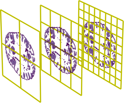
This approach consist of solving a sequence of subproblems with coarser images. These are obtained from the original images by applying a smoothing filter. Starting with the coarsest images we apply the image registration algorithm and then interpolate the obtained solution on the finer domain. One easily observes that the smoother the images are the more regular the problem is and thus providing a higher chance in finding the global solution. Moreover, this approach significantly accelerates and stabilizes the solution algorithm as it provides an excellent initial guess for the current resolution problem.
Here we apply a standard filter based on the stencil described in Section 4.2.1. Let denote the restriction operator to a lower resolution level. Then the overall image registration algorithm is expressed as follows.
Algorithm 2.
Given: original images , integer
Initialize: , ,
- (1)
produce lower resolution images ,
- (2)
set up the image registration problem on the resolution level
- (3)
apply Algorithm 1 to get
- (4)
prolongate
- (5)
update
- (6)
if go to step 1
5. Numerical examples
Next, we present several examples to demonstrate the advantages of our approach. Among the performed tests we consider a tailored example (Ex1) and a real world example (Ex2). The first case is to show how our algorithm works with an ’ideal’ input data, while the second example contains perturbed data requiring some preprocessing.
In order to compare different results we provide two quantitative information, namely the value which approximates the elastic strain energy and which locally measures the distance of the determined deformed image to the reference one.
5.1. Tailored example (Ex1)
Here we demonstrate that our algorithm recovers the true deformation. This example is taken from [19]. Let us define a real function
Now let and set to be uniformly one, i.e., on . Let us define a deformation as
We set to be
The above setting guarantees that the mass preserving constraint is exactly satisfied for the displacement field
On the other hand we know that there may exist other mass preserving solutions with possibly lower elastic strain energy. Therefore we cannot expect that our algorithm produces approximate solutions that converge to . This solution determines an upper bound for the value , namely , where stands for the discretization of , and a lower bound for the dissimilarity measure . We expect to find an approximate displacement with and .
In Figure 2, we present the input data together with the known deformation field and the corresponding difference image. In this example we discretize over a grid of cells.

Further, we calculate
where stands for the computed approximation, to measure how the minimization of influences the solution.
Figure 3 illustrates how the specific properties of the approximated mass preserving solution changes during the optimization process. For comparison purposes, we also depict the results obtained by solving the regularized problem (1) with the dissimilarity measure defined in (2) for different values of the regularization parameter . We call the approximate solution obtained with this method . In this example we skip the multiresolution strategy and stop the iterative solver for the KKT system (14) when the residual norm achieves the tolerance level . The Lamé constants are set to be , .
For tending to zero, both the approximated displacements and exhibit similar properties. Indeed, we see that for , the curves representing the quantities , and (Figure 3 left, middle and right respectively) overlap, which is to be expected.
The main difficulty in the regularized problem is that we do not know the regularization parameter a priori. One can naturally use the L-curve or continuation method [7, 27, 47] in order to find an optimal parameter, but these approaches are rather computationally expensive. In practice, one simply chooses an artificial value. Figure 4 demonstrate how strongly this choice affects the optimization process and the solution. If is chosen too large, we obtain very smooth approximations after few iterations, whereupon the process stagnates and the solution stays far away from . We obtain a reasonably good approximation for . In this situation, however, we must solve extremely ill-conditioned systems. Figure 4(left) presents the required number of iterations for the GMRES solver with algebraic multigrid preconditioner [3]. In Figure 4(right) we present how the regularization affects the obtained deformed image model.
5.2. Real world example (Ex2)
In this example we process real world data obtained from [29]. They illustrate the cortical tissue of human brain at different positions in dimension. The image resolution is . We first apply a Gaussian filter on these images to get rid off the present noise. Then, in order to force the mass preserving condition, we scale these data to get intensity values in range and modify in such a way to obtain the same total mass (sum of all pixel intensities). The value prevents instabilities during the optimization process. We present the input data and the corresponding difference image on Figure 5. We see that the biggest difference appears on the boundary of the cortex tissue. This situation is very realistic and typically comes from spatial misalignment.

We adapt the algorithm to work on free resolution levels, i.e., at each resolution level we stop the iterations as soon as
where corresponds to the cell size at level , which is relative to the cell size at the finest resolution, i.e., , , . As before we set , .
We present the results on Figures 6 and 7. Information from all resolution levels are posed at one figure and separated by vertical dotted lines. Thus we can see the overall performance of the registration algorithm. We can see that is reduced significantly by the solution from the coarser grid and thus justifies the use of the multiresolution strategy. We performed iterations to obtain a solution with the desired DMP tolerance. The regularized problem with parameter , however, does not lead to a solution with and requires in fact a smaller . Figure 7 shows the deformation grid which allows for an almost perfect match of the images, while the mass is preserved with high accuracy.
Remark 6.
We point out that the ratio between the Lamé constants has a big influence on the determined solution. Whenever is large the algorithm allows for solutions that are not divergence-free. On the other hand, when tends to zero, the divergence part of the elastic strain energy dominates. In this situation displacement fields with a dominating divergence-free part are more likely to be chosen.

6. Conclusion
We considered a 2D image registration problem as an optimization problem with a fully nonlinear partial differential equation as a hard constraint. This constraint expresses the preservation of mass while the cost functional controls the linear elastic strain energy of a deformation. We proved that the problem stated in this form has a weak solution in a Sobolev space under fairly mild assumptions. Furthermore, we developed a numerical scheme to solve the problem and demonstrated its robustness on synthetic and real world data. The method involves no regularization parameter and allows to match the images accurately while preserving the mass with high precision.
Appendix A Discretization
A.1. Staggered grid
We assume that the input data and are matrices describing the pixels intensities. We identify each pixel with a square, whose side length is and assume that the given data are associated with the cell centers. The unknown displacements and the corresponding deformations are discretized as follows. Let be the ’th Cartesian axis vector, . We store the variables ( respectively) on the center of grid edges whose orientation is consistent with , where the superscript indicates the discrete approximation. For simplicity let us introduce the following meshes
| (23) | ||||
Moreover, let , , , be appropriate spaces of discrete functions defined on , , and respectively. Additionally we define to be . With this notation we can write , , and . It is worth to note that is the optimization variable and the deformation appears implicitly as , .
Next, we define discrete derivatives of the quantities defined on the staggered grid as
| (24) | ||||
where near the boundary we utilize homogeneous Dirichlet boundary conditions. Observe that with the above second-order accurate definition, the first-order derivatives of a certain quantity in are not collocated with itself. Indeed, one easily notices that , but for . Moreover, locations of the normal and tangential derivatives differ. Such collocation of unknowns and their derivatives calls for introducing projection operators when the constraints are discretized. Therefore we define operators , , as bilinear interpolation, e.g.
| (25) |
A.2. Image model
An important issue is the observation that the input data may have extremely irregular structure. This would lead to instabilities when a numerical method is implemented. In order to minimize the risk of failure there is a need for additional regularization. As one of the building blocks we require a continuous and differentiable representation of the image data . The simplest and computationally cheapest choice would be the linear interpolation method. Clearly the differentiability assumption is then not satisfied. Therefore, following [25] we use the cubic B-spline interpolation scheme [46]. Due to the Curry–Schoenberg theorem [43] we can find a unique B-spline representation of any order for our discrete data . The order 3 is chosen due to the minimum curvature property. With this choice we have the following image model
| (26) |
where is the index related to the control cell containing by the formula , and is the relative position of inside that cell, i.e.,
The functions are the Bernstein basis polynomials of degree . The coefficients may be precomputed. Observe that the continuous function defined in this way possesses smooth derivatives up to third order which can be calculated directly in a simple and computationally efficient way. The B-splines method gives a very good compromise between the accuracy of the interpolation and the reasonable computation time.
Let be a given displacement function and be its corresponding deformation. With this model at hand we can easily calculate the values of and its derivatives at the shifted cell centers
| (27) |
Let denote the warped template image uniquely determined by the displacement and its derivative , i.e.,
where is given as in (27). Then the linear operator being the Fréchet derivative of is
| (28) |
A.3. Constraints
Observe that the constraint contains the Jacobian dterminant , which couples all elements of the Jacobian matrix of . This is in fact the most challenging element to discretize. As mentioned in Section A.1, derivatives are located at different locations. A natural solution would be to apply the projection operator. However, this approach may lead to instabilities as observed in [42]. Therefore, we follow the method proposed in [24]. Instead of discretizing in we calculate the approximated change of volume for each cell. This method is accurate up to second-order and allows to easily detect instabilities [42]. More precisely, let and denote the cell centered at point . Then we have
| (29) |
and the latter is approximated by a procedure precisely described in [24].
Now we define the mapping by
| (30) |
with . From the above discussion, this yields a consistent second-order approximation of the Jacobian determinant [42]. Correspondingly, let denote the Fréchet derivative of at . Similarly, we consider the nonlinear constraint where
| (31) |
Furthermore, its Frechét derivative at denoted by is given by
| (32) |
A.4. Objective functional
Note, that the Fréchet derivative of in is
where is the Laplace operator and denotes divergence operator. A straightforward approach would be to discretize the operator by and define to be as in [28]. This approach, however, has a significant drawback which causes the multigrid method to be inefficient for . Therefore, we choose a mimetic discretization (cf. [20]) in order to preserve the properties of the continuous operator. Let denote the self-adjoint curl operator. Then for any continuous vector field and scalar field we have the identities:
- (i)
- (ii)
- (iii)
Using the property (i) we can write
where denotes the adjoint operator and
Following [20] we assemble operators and satisfying properties (ii) and (iii) on the discrete spaces, and set
| (33) |
Finally, our mimetic discretization of the objective functional reads
| (34) |
whose Fréchet derivative is given by
| (35) |
References
- [1] O. Axelsson and J. Karatson. Efficient preconditioned solution method for elliptic partial differential equation. Bentham Science, 2011.
- [2] R. Bajcsy and S. Kovac̆ic̆. Multiresolution elastic matching. Computer Vision, Graphics and Image Processing, 46:1–21, 1989.
- [3] W. N. Bell, L. N. Olson, and J. Schroder. Pyamg: Algebraic multigrid solvers in python. http://www.pyamg.org, 2013. Version 2.1.
- [4] M. Benzi, G.H. Golub, and J. Liesen. Numerical solutions of saddle point problems. Acta Numerica, 14:1–137, May 2005.
- [5] M. Burger, J. Modersitzki, and L. Ruthotto. A hyperelastic regularization energy for image registration. SIAM Journal on Scientific Computing, 35(1):B132–B148, 2013.
- [6] R. Byrd, F. Curtis, and J. Nocedal. An inexact sqp method for equality constrained optimization. SIAM Journal of Optimization, 19(1):351–369, 2008.
- [7] D. Calvetti, S. Morigi, L.Reichel, and F. Sgallari. Tikhonov regularization and l-curve for large discrete ill-posed problems. Journal of Computational and Applied Mathematics, 123(1–2):423–446, 2000.
- [8] G.E. Christensen, R. Rabbit, and M.I. Miller. Deformable templates using large deformations kinematics. IEEE Transactions on Medical Images, 5(10), 1996.
- [9] N. Chumchob and K. Chen. A robust affine image registration method. International Journal of Numerical Analysis and Modeling, 6(2):311–334, 2009.
- [10] P.G. Ciarlet. Mathematical Elasticity, chapter 1: Three Dimensional elasticity. Elsevier Science Publishers B. V., 1988.
- [11] B. Dacorogna. Direct methods in the calculus of variations. Applied Mathematical Sciences. Springer Berlin Heidelberg, New York, 2 edition, 2008.
- [12] B. Dacorogna and J. Moser. On partial differential equations involving the jacobian determinant. Annales de l’l. Henri Poincaré Analyse non linéaire, 7(1):1–26, 1990.
- [13] A.W. Date. Introduction to Computational Fluid Dynamics. Cambridge University Press, 2005.
- [14] L. Desvillettes and C. Villani. On a variant of korn’s inequality arising in statistical mechanics. ESAIM: Control, Optimization and Calculus of Variations, 8:603–619, 2002.
- [15] L. Evans. Partial differential equations and monge-kantorovich mass transfer - lecture notes. Berkeley, 2001.
- [16] B. Fisher and J. Modersitzki. Fast diffusion registration. Contemporary Mathematics, 313:117–129, 2002.
- [17] B. Fisher and J. Modersitzki. Curvature based image registration. Journal of Mathematical Imaging and Vision, 18(1):81–85, 2003.
- [18] B. Fisher and J. Modersitzki. A unified approach to fast image registration and a new curvature based registration technique. Linear Algebra and its Applications, 23(7):107–124, 2004.
- [19] B.D. Froese. A numerical method for the elliptic monge-ampère equation with transport boundary conditions. SIAM Journal of Scientific Computing, 34(3):1432–1459, 2012.
- [20] F. Gaspar, J. Gracia, F. Lisbona, and C. Oosterlee. Distributive smoothers in multigrid for problems with dominating grad-div operators. Numerical Linear Algebra with Applications, 15:661–683, 2008.
- [21] F. Gigengack, L. Ruthotto, M. Burger, C.H. Wolters, X. Jiang, and K.P. Schafers. Motion correction in dual gated cardiac pet using mass-preserving image registration. IEEE transactions on medical imaging, 31(3):698–712, 2012.
- [22] M.D. Gunzburger. Perspectives in flow controll and optimization. SIAM, Philadelphia, 2003.
- [23] E. Haber, R. Horesh, and J. Modersitzki. Numerical optimization for constrained image registration. Numerical Linear Algebra with Applications, 17:343–359, 2010.
- [24] E. Haber and J. Modersitzki. Numerical methods for volume preserving image registration. Inverse Problems, 20(5), 2004.
- [25] E. Haber and J. Modersitzki. A multilevel method for image registration. SIAM Journal of Scientific Computing, 27(5):1594–1607, 2006.
- [26] J.V. Hajnal, D.L.G. Hill, D.J. Hawkes, and editors. Medical Image Registration. CRC Press, Boca Raton, 2001.
- [27] P.C. Hansen. Rank-Deficient and Ill-Posed Problems: Numerical Aspects of Linear Inversion. SIAM, Philadelphia, 1997.
- [28] S. Henn and K. Witsch. Iterative multigrid regularization techniques for image matching. SIAM Journal of Scientific Computing, 23(4):1077–1093, 2001.
- [29] kkk. Brainweb: Simulated brain database. http://brainweb.bic.mni.mcgill.ca/brainweb. Accessed: 2016-04-14.
- [30] J. Kybic and M. Unser. Fast parametric elastic image registration. IEEE RANSACTIONS ON IMAGE PROCESSING, 12(11), 2003.
- [31] L. Lemieux, U.C. Wieshmann, N.F. Moran, D.R. Fish, and S.D. Shorvon. The detection and significance of subtle changes in mixed-signal brain lesions by serial mri scan matching and spatial normalization. Medical Image Analysis, 2:227–242, 1998.
- [32] F. Maes, A. Collignon, D. Vandermeulen, G. Marchal, and P. Suetens. Multimodality image registration by maximization of mutual information. IEEE Transactions on Medical Images, 16(2), April 1997.
- [33] V.R.S. Mani and S. Arivazhagan. Survey of medical image registration. Journal of Biomedical Engineering and Technology, 1(2):8–25, 2013.
- [34] J. Modersitzki. Numerical Methods for Image Registration. Oxford University Press, New York, 2004.
- [35] J. Modersitzki. Flirt with rigidity - image registration with a local non-rigidity penalty. International Journal of Computer Vision, 76:153–163, 2008.
- [36] Andriy Myronenko, Xubo Song, and Miguel A. Carreira-Perpinan. Non-parametric Image Registration Using Generalized Elastic Nets. In Xavier Pennec and Sarang Joshi, editors, 1st MICCAI Workshop on Mathematical Foundations of Computational Anatomy: Geometrical, Statistical and Registration Methods for Modeling Biological Shape Variability, pages 156–163, Copenhagen, Denmark, 2006.
- [37] J. Nocedal and S.J. Wright. Numerical Optimization. Springer-Verlag, New York, 1999.
- [38] C. Pöschl, J. Modersitzki, and O. Scherzer. A variational setting for volume constrained image registration. Inverse Problems and Imaging, 4(3), 2010.
- [39] T. Rehman. Efficient Numerical Method for Solution of Optimal Mass Transprt Problem. PhD thesis, School of Electrical and Computer Engineering, 2010.
- [40] K. Rohr, H. S. Stiehl, R. Sprengel, W. Beil, T. M. Buzug, J. Weese, and M. H. Kuhn. Point-based elastic registration of medical image data using approximating thin-plate splines, pages 297–306. Springer Berlin Heidelberg, Berlin, Heidelberg, 1996.
- [41] L. Ruthotto. Mass-preserving registration of medical images. Master’s thesis, Fachbereich Mathematik und Informatik, Westfälische Wilhelms-Universität Münster, Deutschland, 2010.
- [42] L. Ruthotto. Hyperelastic Image Registration - Theory, Numerical Methods and Applications. PhD thesis, Fachbereich Mathematik und Informatik, Westfälische Wilhelms-Universität Münster, Deutschland, 2012.
- [43] I.J. Schoenberg and A. Sharma. Cardinal interpolation and spline fucntions v. the b-splines for cardinal hermite interpolation. Linear Algebra and its Applications, 7(1):1–42, 1973.
- [44] S. Suhr. Variational Methods for Combined Image and Motion Estimation. PhD thesis, Fachbereich Mathematik und Informatik, Westfälische Wilhelms-Universität Münster, Deutschland, 2015.
- [45] J.P. Thirion. Non-rigid matching using demons. In Computer Vision and Pattern Recognition, 1996. Proceedings CVPR ’96, 1996 IEEE Computer Society Conference on, pages 245–251, 1996.
- [46] M. Unser. Splines: A perfect fit for signal and image processing. IEEE Signal Processing Magazine, 16(6):22–38, 1999.
- [47] C.R. Vogel. Computational Methods for Inverse Problem. SIAM, Philadelphia, 2002.
- [48] L. Zhu, Y. Yang, S. Haker, and A. Tannenbaum. An image morphing technique based on optimal mass preserving mapping. IEEE Transactions on Image Processing, 16(6), 2007.
- [49] Y. Zhu, E. Sifakis, J. Teran, and A. Brandt. An efficient multigrid method for the simulation of high-resolution elastic solids. ACM Transactions on Graphics, 29(16), 2010.