Classification of planar rational cuspidal curves
I. -fibrationsThanks: This research project has begun as a part of the Homing Plus programme of the Foundation for Polish Science, cofinanced from the EU, and has been finalized as a part of the research project 2015/18/E/ST1/00562, National Science Centre, Poland
Abstract.
To classify complex rational cuspidal curves it remains to classify the ones with complement of log general type, i.e. the ones for which , where is a log resolution of . It is conjectured that and hence is -fibered, where , or is ample on some minimal model of . Here we classify, up to a projective equivalence, those rational cuspidal curves for which the complement is -fibered. From the rich list of known examples only very few are not of this type. We also discover a new infinite family of bicuspidal curves with unusual properties.
1. Main result
All varieties considered are complex algebraic. By a curve we mean an irreducible and reduced variety of dimension . Let be a rational curve which is cuspidal, that is, its singularities are locally analytically irreducible. One can equivalently view as the image of an injective morphism . The literature on such curves is rich (see [FdBLMHN07a] and [Moe08] for a summary). A basic invariant of is the logarithmic Kodaira-Iitaka dimension . Cases with have already been classified (see Lemma 2.14). In particular, their complement is - or -fibered, where .
We will therefore assume that , that is, is of log general type. There are many examples, including several infinite series depending on up to three discrete parameters constructed by various authors, but there is no classification. In fact not many general properties have been proved so far, mostly because the existing theory of log surfaces does not give efficient methods in case . However, recently M. Koras and the first author proved the Coolidge-Nagata conjecture [Pal14], [KP15], which asserts that all rational cuspidal curves are Cremona equivalent to a line. The proof uses, among others, a modification of the Log Minimal Model Program with half-integral coefficients, as developed in [Pal16], and which is based on the generalization of the notion of almost minimality (cf. [Miy01, §2.3.11]). We continue this approach. It turns out that the geometry of is closely related to the geometry of the pair . In particular, we have the following conjecture which strengthens the Coolidge-Nagata conjecture and the Flenner-Zaidenberg Weak Rigidity Conjecture (see Sec. 2B). Put .
Conjecture 1.1 (Negativity Conjecture, [Pal16] 4.7).
If is a smooth completion of a -acyclic surface then . In particular, if is of log general type then it has a -fibration or the pushforward of is ample on some minimal model of .
The -fibration comes as a restriction of a log Mori fibration over a curve of the minimal model of . Note also that is -acyclic. The goal of the current and a forthcoming article is to obtain a classification of rational cuspidal curves (with complements of log general type) up to a projective equivalence, under the assumption that Conjecture 1.1 holds.
Here we work out the most technical part, that is, we classify possible singularities of these for which admits a -fibration. A vast majority of known examples turns out to share this property. It is then no wonder that to achieve a classification we need to go through a detailed combinatorial analysis, even if the general ideas are clear. Let us call an injective morphism with a singular image a singular embedding. We obtain the following geometric description.
Theorem 1.2 (Rational cuspidal curves with -fibered complements).
Let be a rational cuspidal curve with complement of log general type. If is -fibered then one of the following holds (see Fig. 1):
- (a)
is projectively equivalent to one of the Orevkov unicuspidal curves , for some [Ore02, Thm. C].
- (b)
has two cusps and the line joining them has no more common points with , hence is a closed embedding of into .
- (c)
has two cusps and the line tangent to one of them meets in one more point, transversally, hence is a singular embedding of into . The cusp of has multiplicity .
- (d)
is projectively equivalent to one of the Flenner-Zaidenberg tricuspidal curves of the first kind [FZ96, 3.5]. The line through two cusps, including the one with highest multiplicity, has no more common points with , hence is a singular embedding of into . The cusp of has multiplicity .
A detailed classification is given in Theorem 1.3 and we obtain Theorem 1.2 as a corollary. For the definition of Hamburger-Noether pairs, which give a convenient way of describing singularities, see Section 2D. Recall that the Fibonacci sequence is defined by , and .
Theorem 1.3 (Classification of rational cuspidal curves with -fibered complements).
Let be a rational cuspidal curve. Denote by the number of cusps of and by the proper transform of under the minimal log resolution of . Then is a -fibered surface of log general type if and only if the cusps of have one of the following sequences of Hamburger-Noether pairs (the corresponding multiplicity sequences are listed in Table 1):
Case :
- ()
, and for some integers . In particular, and .
Case :
- ()
and for some integers satisfying , and . In particular, and .
- ()
and for some integers satisfying , and . In particular, and .
- ()
and for some integers and . In particular, and .
- ()
and for some integers and . In particular, and .
- ()
and for some integer . In particular, and .
- ()
and for some integer . In particular, and .
- ()
and for some integer . In particular, and .
Case :
- ()
for some integer . In particular, and .
- ()
for some integer . In particular, and .
All the above HN-types are different from each other and each (for every admissible value of , , , , ) is realized by a rational cuspidal planar curve, which is unique up to a projective equivalence.
The HN-type with parameters , will be denoted by . The HN-type with parameters , , will be denoted as , similarly for , and . The HN-type with parameter will be denoted by , similarly for the remaining HN-types. All families except have already appeared in literature. For a detailed discussion see Section 4. The bicuspidal curves are new (see however the discussion in Sec. 4D). As we will see, these are exactly the curves in Theorem 1.2(c). They are geometrically different than other bicuspidal curves listed in Theorem 1.3 in the sense that the line joining the cusps meets . Like all bicuspidal curves above, they are closures of (singular or smooth) -embeddings into , namely the embeddings [BZ10, (b)] with parameters both equal to . However, opposite to other cases, one needs to make a specific choice of coordinates on , different than the one in loc. cit., to obtain them. We explain the construction in Lemma 4.9, see also Section 4.12.
We will address the problem of classification of the remaining rational cuspidal curves (the log del Pezzo case) in a forthcoming article.
Remark 1.4 (Non-standard HN-types).
The HN-types listed above are standard (see Sec. 2D for definitions) except for , , , , , and . We did not convert them to standard HN-pairs to keep some homogeneity of notation. In the first two cases the standard HN-pairs are for the first cusp in , for the second cusp in , for the first cusp in provided and otherwise, for the first cusp in , for the second cusp in , for and for .
As explained above, our approach is based on the Log MMP run for , which strongly motivates the study of -fibrations, as they are related to the log Mori Fiber Space structures over curves (see the remarks after Lemma 2.2). But in the current article the proofs are more elementary in spirit. The list is obtained based mostly on the study of degenerate fibers of the minimal completing -fibration and the interplay with the geometry of the contractible divisor . The key part, classification of singularities, is done in Section 3. First, in Proposition 3.3 we prove in a constructive way that one may choose a -fibration of which has no base points on the minimal log resolution. Interestingly, this property holds for all -homology planes of log general type which admit some -fibration (an analogue for -fibrations holds too, see Proposition 4.2). We note here that many results on fibers of -fibrations of -homology planes have been proved in [MS91]. However, we need a much more detailed analysis. Then, given the extension of the fibration to , we study the specific cases when contains a full fiber (Lemma 3.5) or a multiple section (Lemma 3.6, Corollary 3.7). The case into which most of the curves fall is when contains three sections but no full fiber. To obtain a classification in this situation we show that there are at most three degenerate fibers and all of them are rational chains (Lemma 3.9), and then that one may assume is vertical (Lemmas 3.11 and 3.14). We use also the results of Tono, who analyzed some special cases (, and , , see Lemma 2.17).
In Section 4A we show that, conversely, if is of one of the HN-types listed in Theorem 1.3 then its complement is -fibered and of log general type. Finally, in Sections 4B - 4D we prove the existence and uniqueness of curves of each HN-type listed in Theorem 1.3. For families and , this result follows from the original constructions [FZ03, Ore02]. We prove that the curves of HN-types - arise as closures of embeddings of into and we show how to deduce their uniqueness from the classification of such embeddings obtained in [CNKR09, KP16]. The existence and uniqueness of the new curves of HN-types is proven in Lemma 4.9.
2. Preliminaries
2A. Log surfaces.
For a smooth projective surface we denote by the Néron-Severi group of Cartier divisors on modulo numerical equivalence. Put and . A smooth rational projective curve on with is called an -curve. By the adjunction formula for such a curve, where denotes the canonical divisor.
Let be an effective divisor on . By a component of we always mean an irreducible component of (not a connected component). The number of components of is denoted by . We call a simple normal crossing divisor (snc for short) if its components are smooth and its only singularities are nodes. We call a smooth pair if is a smooth projective surface and is a reduced snc-divisor on . For every effective divisor on there is a sequence of blow-ups , such that the total transform of is snc: such a process is called a log resolution of singularities. For every smooth surface there exists a smooth pair , such that . Every such pair is called a smooth completion of . If is a smooth pair with then a blowup at a point is called outer for if is a smooth point of , otherwise it is inner for .
Assume that is a reduced snc-divisor. A dual graph of has vertices representing components of with weights being their self-intersection numbers, and an edge between two vertices represents a point of intersection of the corresponding components. If is an effective subdivisor of we define its branching number as:
If is a component of with we say that is a tip of . If we say that is branching in . We say that an effective snc-divisor is a tree if the dual graph of is connected and contains no loop. Further, is a rational tree if additionally all components of are rational curves.
A rational tree with no branching component is called a chain. It is ordered if it has a distinguished first tip. If is ordered and reduced we can write , where ’s are irreducible and (hence for ). Assuming is the distinguished tip of we write also , where . If we write for the same chain with opposite order. If a rational tree has only one branching component and then is called a fork.
An effective subdivisor of an effective divisor is called a twig of if it is a chain with components , such that and . By convention we assume that is ordered so that the tip is its first component. A twig is maximal if it is maximal in the set of twigs ordered by inclusion of supports.
A -curve in is called superfluous if it intersects at most two components of , each in one point and transversally. Equivalently, after its contraction the image of is an snc-divisor. An snc-divisor is snc-minimal if it has no superfluous -curves.
We put and for a nonzero reduced divisor with components we put . Elementary properties of determinants imply the following:
Lemma 2.1 (discriminants).
Let be a smooth pair.
- (a)
Let be a blowup of a point on , where is the reduced preimage of . Then . In particular, if contracts to a smooth point then .
- (b)
Let and be reduced snc-divisors on for which and let , be the unique components of and which meet. Then:
Following [Ton12a], for two chains , we put . We have for chains . If is a chain we define . It is easy to see that a chain can be contracted to a -curve if and only if . Moreover, in the latter case (see [Fuj82, 4.8]).
Let be a birational morphism between smooth projective surfaces. Then we can write as a composition of blowups for some . If is a curve on then we say that a blow-up does not touch if it is an isomorphism in some neighborhood of . We say that touches times for some if exactly of the blowups touch and each exceptional divisor meets the respective proper transform of transversally in one point. Note that in this case .
2B. -acyclic surfaces and related conjectures.
If is a rational cuspidal curve then by the Poincaré-Lefschetz duality [Bre93, 8.3] the surface is -acyclic, that is, the Betti numbers vanish for . All smooth -acyclic surfaces are affine [Fuj82, 2.5] and rational [GP99]. By the work of many authors -acyclic surfaces which are not of log general are classified (see [Miy01, §3.4]). The case of log general type is much more complicated. We need the following result.
Lemma 2.2 (No affine lines, [MT92], [Miy01] II.3.1).
A smooth -acyclic surface of log general type contains no curves isomorphic to . In particular, every its smooth completion for which is snc-minimal is almost minimal.
We note that this result uses the logarithmic version of the Bogomolov-Miyaoka-Yau inequality. Almost minimality means that when passing to the minimal model of in the sense of Mori we contract only curves contained in and its images. Unfortunately, even in case is of type this fact gives rather weak restrictions on the singularities of .
In this situation, the first author proposed studying the minimal model of . In [Pal16, §3] he described the creation of the latter and made the Negativity Conjecture 1.1 for -acyclic surfaces, which is in fact the main motivation for the current article. This conjecture implies the Flenner-Zaidenberg Weak Rigidity Conjecture [FZ94] (equivalent to the vanishing of ; see [Pal16, 2.5(2)] for a discussion), and hence the Coolidge-Nagata conjecture. It is better suited for the log MMP approach. For instance, once it is proven, the log MMP for implies that some minimal model of has a structure of a Log Mori Fiber Space. If the base is a point then the pushforward of is ample on it. If the base is a curve then, since the general fiber is isomorphic to , we get that , so , and hence , as otherwise would not be of log general type. The latter fibration induces a -fibration on , where .
2C. -fibrations.
A -fibration of a smooth projective surface is a dominating morphism with general (scheme-theoretic) fibers isomorphic to . A fiber non-isomorphic to is called a degenerate fiber. All fibers of are numerically equivalent and have self-intersection . Conversely (see [BHPVdV04, V.4.3]), for any -curve on or, more generally, for any effective divisor with and , there is a -fibration of with as one of the fibers.
For a given -fibration with general fiber , we say that an (irreducible) curve is vertical (resp. horizontal) if (resp. ). Every divisor can be uniquely decomposed as , where all components of are vertical and all components of are horizontal. A horizontal curve with is called an -section. If is vertical and irreducible then by we denote the multiplicity of in the fiber containing ; such a fiber will be usually denoted by .
Every degenerate fiber of a -fibration can be contracted to a -curve by iterated contractions of -curves. Therefore, by induction one easily gets the following (see [Fuj82, 4.14]):
Lemma 2.3 (Degenerate fibers).
Let be a degenerate fiber of a -fibration of a smooth projective surface. Then is a rational tree and its -curves are non-branching in . Furthermore:
- (a)
If a -curve is a component of and then and contains another -curve.
- (b)
Assume that has a unique -curve and let be the connected components of . Let , be some fixed components of and respectively. Then:
- ()
If and then are tips of and is a chain . Moreover, .
- ()
If and then either is a chain like above, or is a fork with maximal twigs , and , such that is the first tip of and contracts to a smooth point (see Fig. 2).
- ()
- (c)
Assume that contains only two -curves and , and both connected components of contain components of multiplicity . Then is a chain of type for some .
Figure 2. A special fork from Lemma 2.3. The tips are the only components of multiplicity ; .
A fiber like in Lemma 2.3() will be called a special fork.
Assume that is a smooth quasi-projective surface. A morphism to a smooth curve is called a -fibration if there exists a nonempty Zariski-open subset , such that for every there exist points , such that the scheme-theoretic fiber is isomorphic to . Call the maximal subset of with the above property. A fiber for is called a degenerate fiber of .
For a -fibration there exist smooth completions of and of , such that extends to a -fibration with for every fiber of . Any triple as above will be called a completion of a fibration . We will use the following:
Notation 2.4.
Let be a smooth pair and a -fibration. Then is the number of horizontal components of , is the number of fibers contained in and for denotes the number of components of not contained in .
Lemma 2.5 ([Suz77, 9.2], [Zai87, 3.2], cf. [Miy01, III.1.8]).
Let be a smooth affine surface and let be a -fibration with general fiber . Then:
- (a)
For every degenerate fiber of we have and if the equality holds then or .
- (b)
Lemma 2.6 ([Fuj82, 4.16], cf. [Pal15, Lemma 2]).
Let be as in Notation 2.4. Then:
In particular, if the components of generate freely, e.g. when is -acyclic, then
In order to apply Lemma 2.5 to -fibrations we need the following:
Lemma 2.7 (Curves with ).
Let be a, possibly reducible, affine curve such that . Assume that contains no component homeomorphic (in the complex topology) to , such that consists of at most one point. Then is a disjoint union of curves homeomorphic to .
We argue by induction on . The case is obvious. Let be a component of intersecting in points. We have for some , where is a projective curve. Let be its normalization. We have
hence . Moreover, the inequality is an equality if and only if , and , that is, is homeomorphic to , so in this case by assumption. It follows that in every case
Thus by the inductive hypothesis is a disjoint union of curves homeomorphic to . Then , so and the argument above implies that the inequality is strict. Thus , is homeomorphic to and is disjoint from , as claimed. ∎
Corollary 2.8 (-fibrations).
Let be a -fibration of a smooth -acyclic surface of log general type. Then, with the notation as in Notation 2.4:
- (a)
has degenerate fibers, each of them is disjoint union of curves isomorphic to ,
- (b)
, where the sum runs over all degenerate fibers of ,
- (c)
.
(a) Let be a minimal completion of . Since is rational, is isomorphic to an open subset of with . The closure of a fiber in is a rational tree. By Lemma 2.2 has no component isomorphic to and by Lemma 2.5(a), . Then Lemma 2.7 shows that every degenerate fiber is a disjoint union of ’s. By Lemma 2.5(b) , so .
(b) Because the components of generate freely, from Lemma 2.6 and part (a) we have .
(c) If are fibers contained in then the linear equivalence implies that the components of are not linearly independent in , hence the natural homomorphism is not surjective, so by the Poincaré-Lefschetz duality ; a contradiction. ∎
Note that if is a minimal completion of then the closure of a non-degenerate fiber of is a non-degenerate fiber of , which follows easily from the fact that none of the components of contained in the completed fiber can be a -curve. On the other hand, a completion of a degenerate fiber of may very well be a non-degenerate fiber of .
2D. Log resolutions and Hamburger-Noether pairs.
The are many ways of describing the geometry of cusps and exceptional divisors of their resolutions. We use the Hamburger-Noether pairs (HN for short), because on one hand they are a compact way of keeping track of sums of multiplicities and squares of multiplicities of singular points on successive proper transforms of the cusp and on the other hand they are directly related to weights of dual graphs (see Lemma 2.12). For more details we refer the reader to [KR99, Appendix] and [Rus80]. The relation with the multiplicity sequence is explained in Lemma 2.11. Relations with other numerical characteristics (Puiseux pairs, Zariski pairs) are explained in Section 5.
Let be an analytically irreducible germ (a cusp) of a planar curve singular at the point . Let be the exceptional divisor of its minimal log resolution and let be the unique -curve in intersecting the proper transform of . Since is created from a smooth point by a sequence of blowups, its structure is easy to understand. For instance, every component of meets at most three others and if it meets three then it meets a maximal twig of (see Fig. 3). Since the log resolution is minimal, is not a tip of .
Letting vary through smooth germs at , we note that the intersection numbers at are bounded from above. Any smooth germ for which the maximum is reached is said to be maximally tangent to at . We denote the multiplicity of the singular point by .
For the beginning of the induction let be a smooth germ maximally tangent to . For the inductive step assume we are given a triple such that and are respectively an analytically irreducible and a smooth germ of planar curves. If is smooth and meets transversally then we stop, otherwise we put and we choose a smooth germ transversal to at and such that
| (2.1) |
We put . We now blow up over until the proper transform of intersects the total transform of not in a node and we denote by the last exceptional curve. This way we obtain a sequence
of the standard HN-pairs of the cusp . By the Euclidean algorithm and by the transversality of we get for
| (2.2) |
respectively. Our choices of and give respectively
| (2.3) |
With these choices the sequence of HN-pairs is unique and has exactly branching components. One can also show that with the convention (2.1) has exactly Puiseux pairs, see Lemma 5.1.
Example 2.9 (Semi-ordinary cusps).
A cusp of HN-type for is called semi-ordinary. It has multiplicity and is locally analytically isomorphic to the singular point of at . The exceptional divisor of its minimal log resolution is a chain . It is often called a cusp of type . A semi-ordinary cusp for (type ) is called ordinary.
Remark 2.10 (Non-standard HN pairs).
It is possible, and in some situations more convenient to allow more general choices of or for which do not satisfy (2.3) (running inductive arguments more smoothly is one of the reasons). For instance, instead of (2.3) we could ask to satisfy (as it is done in [KPR16]), which results in replacing all pairs where with sequences , where is the integer part of and means repeated times. Additionally, we could allow a more general choice of , which will relax the condition . Converting the so-computed non-standard HN-type to the standard one results with replacing the initial part
| (2.4) |
The reader can check that this does not affect the basic equations listed in Lemma 2.13. In particular, it is sometimes convenient to replace the initial germ with the germ of the line tangent to at the cusp. We we will use such tangent HN-types in future articles. Note however, that although they carry more information than the local topology of the singularity, they makes sense only for planar projective curves.
The multiplicities of the preimage of on the proper transforms of under consecutive blowups form the multiplicity sequence of . Since we rely on HN-pairs, we need a recipe to compute one from another. For examples see Table 1.
Lemma 2.11 (HN-pairs vs the multiplicity sequence).
Let be an analytically irreducible germ of a planar curve.
- (a)
Let be some HN-pair which is an element of some (not necessarily standard) HN-sequence of . Then the part of the multiplicity sequence of corresponding to this HN-pair is
where, putting , the numbers and for are respectively the quotient and remainder of dividing by . The index is the first such that .
- (b)
Let with be the multiplicity sequence of . Then is of standard HN-type
where for are defined inductively as follows: ; if then we put and we stop. Otherwise we put , where is the unique integer such that .
(a) Blow up once on . If this is the end of the sequence of blowups described by , so the claim is clear. We may assume, say, . The remaining sequence is described by the HN-pair , which is a part of some sequence of HN-pairs for the proper transform of . The result follows by the Euclidean algorithm.
(b) Let be the standard HN-type of . By assumption and . Blow up times over . The proper transform of has (not necessarily standard) HN-type , so .
The formula for , holds by (2.2). Fix . We perform the sequence of blowups described by and part of until the multiplicity of the cusp drops to . We have and the intersection of the proper transform of with the last exceptional curve equals . Then we do the remaining blowups, each time the multiplicity of the center is , until the proper transform of does not meet the total exceptional divisor in a node. At this point, by the definition of HN pairs, we have a smooth germ transversal to the last exceptional component , and , are respectively the intersections of with and with . If then , so and hence , so we are done. We may therefore assume . After further blowups the multiplicity of the cusp drops to . Because it drops, the intersection of the proper transforms of and , which is , is smaller than . Since is maximally tangent to , we have . Indeed, otherwise the image of any germ transversal to the last exceptional component and meeting the proper transform of the cusp would be a smooth germ with a bigger intersection with than . We infer that the multiplicity of the cusp is , so and we are done. ∎
We have the following useful description of the graph of in terms of HN-pairs:
Lemma 2.12 (Dual graphs from HN-pairs, [Pal14, 3.5]).
Let be the chain created by the characteristic pair with and let be the unique -curve of . Write , where and are disjoint and connected, with . Put if . Let be the tips of which are components of and , respectively. Write for some integers and . Then:
Lemma 2.13 (Equations for HN-pairs, [Pal14, 3.3]).
Let be a rational cuspidal curve with cusps , where is described by a sequence of HN-pairs . Let be the minimal log resolution and let be the proper transform of on . Put , and . Then
- (a)
,
- (b)
- (c)
.
Note that the last formula is the genus formula written in terms of HN-pairs.
2E. Some upper bounds on .
We have the following criterion:
Lemma 2.14.
For a rational cuspidal curve the following conditions are equivalent:
- (a)
,
- (b)
is - or -fibered,
- (c)
contains a curve isomorphic to .
The implication (a)(b) is obtained in [Pal16, 2.6] as a corollary from the existing structure theorems for affine surfaces which are not of log general type (an additional argument is required in case ). The implication (b)(c) follows from Lemma 2.5. The implication (c)(a), based on the logarithmic BMY inequality, follows from Lemma 2.2. ∎
In fact there is a detailed classification of rational cuspidal curves with . The case was shown to be impossible in [Tsu81]. The case was treated in [MS81] and [Kas87]. The case was treated in [Ton01] and [Ton00]. We note that one could recover the classification in a more unified manner starting from the equivalence (a)(b) above.
Notation 2.15.
Let be a rational cuspidal curve with cusps . By the above discussion we may and shall assume that . We denote by the minimal log resolution and by the proper transform of on . Then contains a unique -curve intersecting , which we denote by .
Lemma 2.16 (Upper bounds on , Tono).
(a),(b) Assume the contrary. Blow up over until the proper transform of has self-intersection if and if . Call the last exceptional curve of the blow-up, or put if no blow-ups were needed. If then induces a -fibration which restricts to a - or -fibration on . Similarly, if then so does . Then by Iitaka’s Easy Addition Theorem; a contradiction.
(c) Let be a divisor on a smooth projective surface and let be a blowup at a point of multiplicity on . Put and . Then:
| (2.5) |
Recall that the blowups with and are called respectively outer and inner (for ). Let be the standard sequence of HN-pairs for the cusp and let denote the biggest integer not greater than . Blowups constituting the log resolution of other than the first one are either inner or outer and there are exactly outer ones among them. Since , by (2.5) we get:
Vanishing theorems for cohomology imply that (cf. [Ton12c, 2.7])
hence the above inequality gives , as claimed. ∎
For the boundary values of there is already a classification available.
Lemma 2.17 (Cases , Tono).
With the notation as in 2.15 we have the following bounds:
- (a)
If has only one cusp and then has HN-type or .
- (b)
If has exactly two cusps and then has HN-type - with .
3. Possible types of cusps
In this section we prove the following proposition. We use the notation of Section 2C.
Proposition 3.1.
Assume that is a rational cuspidal curve such that is -fibered and of log general type. Then is of one of the HN-types listed in Theorem 1.3.
Note that if the HN-pairs are known then and are determined by Lemma 2.13.
3A. Reduction to fibrations with no base points.
The example below shows that a -fibration of can have base points on the minimal log resolution .
Example 3.2 (A -fibration with a base point.).
Let be the Orevkov curve of degree (type in Theorem 1.3). The graph of is shown in Figure 4. Denote by and the long and short maximal twigs of contained in . Denote by , respectively the first and the last tip of and by , the first and the last tip of . Assume that there exists a -curve with meeting in and in . Call the -chain of type in containing . Let be the blow up over . Consider a -fibration induced by the proper transform of : it restricts to a -fibration of which has base points on .
It remains to prove the existence of . Let be the -fibration induced by . Then and for any fiber of . By Lemma 2.6 the fiber of containing has at most two components not in . Let be such a component. Since is connected and contains no loop, . By Lemma 2.2 , so we get . If meets then since ; similarly if meets then since and meets . By Lemma 2.3(c) . Let be the tip of meeting . If meets then on we have , which is impossible. Hence meets as claimed.
The following reduction constitutes an important step in the proof of 1.3.
Proposition 3.3 (Reduction to -fibrations with no base points).
Let be a smooth snc-minimal completion of a smooth -acyclic surface of log general type. If has a -fibration then it has a -fibration without base points on .
Let be a -fibration of and let be the minimal resolution of base points of on . Let be a -fibration of which restricts to and let be a fiber of . Recall that by the Poincaré-Lefschetz duality , so the long exact sequence of homology for the pair shows that , hence is a rational tree.
Claim.
Let be a composition of some number of contractions of -curves in and its images. Put , . Then for every -curve of we have and if .
Suppose that . We may assume is a degenerate fiber. Since , we have . We have also , so . The divisor is a rational tree and the divisor is a sum of rational trees. By Lemma 2.2 the tips of the latter divisor which do not meet are contained in . Since is affine, is connected (see [Har77, p. 244]), which implies that . Since , , and hence , contains a -curve. The latter is non-branching in , so is not a minimal resolution of base points; a contradiction.
Now suppose that and . Then . Again, , so by Lemma 2.3 contains a -curve . We can assume that consists of blow-ups over points of . Indeed, if , where consists of all the connected components of which meet the proper transform of on , then we can decompose as in such a way that and . Then does not touch , hence if the claim holds for , it holds for as well. Suppose touches . Then , hence . We have , because otherwise , contrary to Lemma 2.2. The divisor contains a -curve with , hence . By the minimality of this -curve is not a component of . We get and by Lemma 2.2. Since is a tree, it follows that is not connected. But is affine, so is connected, which implies that every connected component of meets . Since , this means that ; a contradiction.
Therefore, does not touch . Suppose . Then the proper transform of on is a -curve in , necessarily branching by the minimality of , so . We get and by Lemma 2.3. Because , we get , so is non-branching in ; a contradiction. Thus and then by Lemma 2.2. Since is connected, every connected component of meets , so . Because is a tree, meets each connected component of at most once, which gives . We obtain ; a contradiction. ∎
Suppose that . Note that has at least one degenerate fiber. Indeed, and we have , because otherwise is a planar curve of degree at most , contrary to the assumption . Let be the last exceptional curve of . Since is snc, is non-branching in . By the minimality of , is horizontal. Contract -curves in and its images until some component meeting , call it , becomes a -curve. Let be the resulting morphism. Put , and .
Suppose . We have . If is a component of then by the claim above , so . Thus and by the claim above . Since is a tree, meets each connected component of at most once, so , which means that meets two connected components of , and hence that . Since is connected, every connected component of meets , hence ; a contradiction.
So we proved that . Then , which means that the intersection of with a general fiber of the -fibration of induced by the linear system is at most three. Since is an open subset of , it is of log general type, so by Iitaka’s Easy Addition Theorem [Iit82, 10.8] we have in fact . Call the contraction of . Then is a smooth pair and the image of induces a -fibration of which restricts to a new -fibration of . For this -fibration the minimal resolution of base points on is shorter than . Thus the lemma follows by induction on the length of . ∎
3B. Cases with a fiber at infinity.
From now on to the end of this section we assume that is a rational cuspidal curve, such that is -fibered and of log general type. We keep the notation 2.4 for -fibrations and 2.15 for resolutions. By 3.3 we can choose a -fibration of which extends to a -fibration of . Moreover, by Lemma 2.16 and Lemma 2.17 we may and shall assume that:
| () |
Notation 3.4 (Figures of dual graphs).
Throughout the proof we present weighted graphs of for curves of the HN-types listed in 1.3 together with -fibrations on restricting to -fibrations on . Verification of correctness of the weights is always a straightforward computation based on Lemma 2.12. The convention for figures of these graphs is as follows. The horizontal line represents . Bold lines represent horizontal components of . The dashed lines represent components of degenerate fibers which do not lie in . The numbers near the lines are the self-intersection numbers of respective curves. As before, we write for a chain consisting of -curves. To avoid the necessity of treating some special cases separately, we use the notation and .
We will now prove a few lemmas reducing the proof of 3.1 to some special situations. Let us first make a general remark. Namely, if the -curve is vertical for then by Lemma 2.3 , so . Thus if is vertical for then
| (3.1) |
In particular, meets .
Lemma 3.5 (Cases with a fiber at infinity).
Assume that contains a fiber of and that is not of HN-type , or . Then there is a -fibration of which has no base points on and whose completion has no fiber in .
Let be a fiber of contained in .
Claim 1.
contains and is of type . In particular, and .
By ( ∗ ‣ 3B) , so contains no -curves. It follows that is degenerate, so it has a -curve . Since ’s are the only -curves in , we have, say, . Because ’s are negative definite, contains .
By (3.1) for every vertical , so since , we infer that is the unique -curve of and hence that . The latter implies that if is not a chain then is a tip of , so and , which is false. Thus is a chain. Since , we get or .
Suppose that . Then by Claim 1, so . We have , so is a -section, hence and . Moreover, contains a tip of . It follows that the last HN-pair of is for some , so (using the notation of Lemma 2.13) and hence Lemma 2.13(a) fails. Thus . By ( ∗ ‣ 3B) and . Then and . ∎
The curve is a -section meeting . Let , be the connected components of . Since they both meet the -section , they lie in different fibers , respectively. By 2.8(a) has two degenerate fibers, so has at most two degenerate fibers other than . These are necessarily and , so by 2.8(b) we have and . Denote by , and by the components of and respectively which are not contained in .
Claim 2.
is a chain and we may assume meets it in tips.
Since is a rational tree such that is a disjoint union of two ’s, the set has exactly three connected components (some of them may be points). Because of the connectedness of , each of these connected components meets , hence either belongs to (if it is a point) or contains a component of multiplicity . Since contains no -curves, this can happen only if is a chain.
Call the component of meeting . Assume is a tip of . Say that meets . Since is a tip we can perform inner contractions in starting with until the image of is a -curve. Call the resulting morphism. It contracts only components of multiplicity bigger than , so it does not touch . We get
Then induces a -fibration of which restricts to a -fibration of (it cannot restrict to a -fibration because by assumption ). For this new fibration is a section, so by Claim 1.
Hence we can assume that is not a tip of . Then components of of multiplicity lie in or are tips of , so meets in tips; see Fig. 5. ∎

Claim 3.
We may assume is connected.
Assume is not connected. Then it has a connected component meeting . By Lemma 2.3 is either a chain or a special fork. Since , it follows that meets at least one of ’s, say . Let be the connected component of other than (there is only one, because ). If meets then induces a -fibration of as needed. Hence we can assume that for every , meeting . It follows that . Indeed, if then by Lemma 2.3(c) consists of -curves, so by the negative definiteness of , is a tip of , so some meets and , contrary to the assumption.
Consider the case when is a chain. Then meets in a tip and meets in a component with . Suppose that . Because contracts to a smooth point, contracts to a smooth point too, so we have for some and hence for some . Note that meets in a tip, for otherwise would be a branching -curve in meeting , which is impossible, as contracts to a smooth point. Since , meets , so . Then he contractibility of gives or for some . Thus or . In any case, we check that does not contain a component of multiplicity in ; a contradiction. Therefore, and since , we have and for some . As before, is a tip of , for otherwise the contractibility of would imply that is a -chain, which is false. Hence meets . Then is a chain, so since it contracts to a smooth point, or for some . From the form of we get . But since contracts to a smooth point, should contract to a smooth point, and it does not, because and are not coprime; a contradiction.
Now consider the case when is a special fork and is a chain. Then , for some and the component meeting is a tip of . Since is not a -chain, the contractibility of implies that is non-branching in , hence it is a tip of and then again it meets . Then is a chain, so we get or for some . On the other hand, since , the contractibility of implies that for some , so because contracts to a -curve, we get for some ; a contradiction.
Finally consider the case when is a special fork and is fork. Since contracts to a smooth point, the long twig of is necessarily for some . Then and the branching component of is a -curve for some . The contractibility of implies also that is a tip of and , so because contracts to a -curve, we get . Since contracts to a smooth point, we get . But then , so ; a contradiction. ∎
By Claim 3 and Lemma 2.3(b), is a special fork and consists of -curves. Since contracts to a smooth point, is necessarily a chain, so ; see Fig. 6. Assume that is connected. Then by Claim 2 is a chain, so the contractibility of to a smooth point implies that and for some . Hence for some . Because contracts to a smooth point, we have , so . It follows that is of HN-type , . Since , from Lemma 2.13 we get . Thus is of HN-type .
We can therefore assume that is not connected. Write , where is the contraction of and is the tip of meeting . Put . Because , the morphism is a minimal log resolution of the bicuspidal rational curve . Since does not touch , we have . By Lemma 2.17, is of one of the HN-types - with . But one of the cusps of has one HN-pair, because the respective exceptional divisor is a chain, and the second one has two HN-pairs, the second being , because . It follows that is of HN-type or for some . The resulting HN-pairs are and for HN-type and and for HN-type , (for the latter sequence degenerates to ). Then the HN-pairs for are and for HN-type and and for HN-type (degenerating to for ), which are exactly the HN-pairs of (Fig. 8) and (Fig. 8). ∎
3C. Cases with two horizontal components.
By Lemma 3.5 from now on we may and shall assume that contains no fiber of , that is, . From Lemma 2.6 we get .
Lemma 3.6 (Cases with two horizontal components in ).
If then we may choose so that it has no base points on , contains no fiber of and is a -section of .
Since and , by Lemma 2.6 every degenerate fiber has a unique component not in . We can write , where is a -section and is a section of . Moreover, by Corollary 2.8 has exactly two connected components for every degenerate fiber (one of them could be a point) and each of them has a unique common point with .
Suppose is not a -section of .
Claim 1.
is vertical.
Suppose that . Then is not vertical. Indeed, otherwise , since , and then could not meet , which is a -section. Thus every contains a component of and hence . If there exists a degenerate fiber which does not contain then is its unique -curve and does not meet , so meets , which gives , contrary to Lemma 2.3(b). Hence has a unique degenerate fiber and this fiber contains . Because meets , we have , so is a tip of and by Lemma 2.3(a) is a -curve.
Contract and the new -curves appearing in the subsequent images of . Call the resulting morphism. Since contracts the unique degenerate fiber of to a -curve, is a Hirzebruch surface for some . Since , we see that meets , so meets in components on multiplicity , it is therefore not touched by inner blow-downs in and its images. It follows that is a smooth rational -section on and, since is the only component of meeting , is a -section disjoint from . This is possible only if and . But does not touch , so ; a contradiction with Lemma 2.16(a). ∎
Call the fiber containing . If is not connected, denote by the connected component of not containing , otherwise put . Put .
Claim 2.
We may assume that is vertical and .
Suppose that all ’s are horizontal. Then contains no -curves, so for every degenerate fiber , is the unique -curve in . In particular, . Since , is a tip of and meets . Let be the component of meeting . We have and . We have also .
Suppose that . By Lemma 2.3(b) is a special fork and meets only in , hence . Therefore, by ( ∗ ‣ 3B) . Then is a fork with two twigs of type , one of which is , and the third twig meeting in a tip. It follows that meets the last exceptional component of , so is a -curve on ; a contradiction.
Thus . Now , so and is a tip of . If then some , say , meets , so induces a -fibration of such that is a -section. But then , being contained in , is negative definite, so , hence this -fibration restricts to a -fibration of as needed.
We may therefore assume that . If is a -section then meets both and , so is a branching -curve in which meets a -curve . Since contracts to a smooth point, this is possible only if is a tip of , and this is not the case. So is a -section. Then meets the -section , so . If then meets two -twigs of , which is impossible, as is negative definite. Hence . In particular, .
Let be the connected component of not containing . We can write as where and disjoint and connected (possibly zero divisors), meets and and meets . Then are connected components of ; see Fig. 9. Suppose . Then . Call the fiber containing . Since , we have , and hence , so contains . Then both and intersect in components of multiplicity , so by Lemma 2.3 is a chain of the form and meets it in tips. Since contracts to a smooth point, we have for some , hence . The last tip of is the unique component of of multiplicity , so it meets . Then this tip of is a branching -curve of , so the contraction of makes it into a curve of non-negative self-intersection, which contradicts the negative definiteness of .
Hence and meets . Suppose that . Let be the fiber containing . Since , and hence contains . We have , so since contracts to a smooth point, for some . By Lemma 2.3(b) is a chain, so and . But then ; a contradiction with .
Hence . Then . Call the fiber containing . Since is connected, meets . By Lemma 2.3 is a special fork and consists of -curves. Since contracts to a point, and hence . Then is of type and Lemma 2.13(c) fails; a contradiction.
Thus we may indeed assume that is vertical. It remains to show that . If is vertical then it is contained in and by (3.1) . Since , we see that is the only vertical . Since , we get . But if then , so the connected component of not containing has no common points with ; a contradiction. ∎
By ( ∗ ‣ 3B) . Note also that contains no -curves other than , so for every degenerate fiber the curve is the unique -curve in . In particular, and hence . Recall that denotes the connected component of not containing and in case we denote by the component of meeting .
Claim 3.
with as the second curve.
Suppose is a tip of . Because , meets both and . Since , after the contraction of the curve is the unique -curve in the image of . It follows from Lemma 2.3 that , so and is a tip of .
Suppose that . Let be the connected component of meeting only in and let be the fiber containing it. We have for . Since is the unique -curve in , the multiplicity of is at least , so we get . Then intersects in a component of multiplicity and, since , contains a connected component of , which meets only in . Because of the contractibility of to a smooth point, is a chain of -curves. It follows that is not a chain, because otherwise is irreducible, and hence would not have multiplicity , as required. By Lemma 2.3 is a special fork. But then, since is a -chain, we have , so ; a contradiction.
Thus . If does not meet then because of the contractibility of we have either and or and . In the first case Lemma 2.13 fails and in the second is a -curve on , which is impossible. Hence there is a connected component of meeting only in the -section . If there are in fact two such connected components but they lie in different fibers of . This means that is connected, so by Lemma 2.3 is a special fork and consists of -curves. Since is contractible to a smooth point, it follows that and that is a chain meeting in a tip. Moreover, one of or is a -curve. If then is a -curve on and if then and is of HN-type , so Lemma 2.13 gives ; a contradiction.
Thus we proved that is not a tip of . We infer that there is a component of meeting and hence that . By (3.1) , which gives and . Let be the contraction of . Then the connected component of meeting contains two components of multiplicity in , namely and . we have , so if is not a -curve then is a unique -curve in and hence . But in the latter case meets and hence also contains a component of multiplicity , which is impossible by Lemma 2.3. Therefore, is a -curve, necessarily unique in . Since , is a tip of . The -section meets some component of of multiplicity . It follows now from Lemma 2.3 that , and hence that . ∎
As above, denote by the tip of contained in . Clearly, meets only in and meets in the tip contained in , because it is the only component of of multiplicity . Since , there are at most three connected components of meeting , call them , and with meeting and , meeting only in . If then is one of these connected components, that is . Now may have one more connected component , which meets only in ; see Fig. 10. As usually, we call the fiber of containing , where is one of , , or .
Claim 4.
and . Moreover, contains .
Suppose , that is, . Both and meet , so . It follows that does not meet and hence contains and meets it in a component of multiplicity . By Lemma 2.3 is a chain meeting in tips (which are unique components of multiplicity ). It follows that and meet the same component of . If is irreducible then . On the other hand, if is reducible then the contractibility of to a smooth point implies that for some and hence that . In both cases the contraction of maps onto the chain of discriminant . This is a contradiction, because is negative definite.
Now suppose . In case we can assume, renaming and if necessary, that also . Now meets only in and and either is a tip of or and . We have , so is connected. If then by Lemma 2.2 , so for some we have , which is in contradiction to Lemma 2.3. So and hence is a chain. Since contracts to a smooth point we have . Then is a -curve on ; a contradiction.
The fibers and have unique -curves and these -curves have multiplicity at least . If then, since meets , we have , so is not connected, so in any case . Note also that if then , so since the affine part of the fiber is isomorphic to , meets in a unique point belonging to a component of of multiplicity . Call this component .
Suppose that , equivalently, that . The -section meets in some component of multiplicity , so by Lemma 2.3 is a chain or a special fork. Since contracts to a smooth point, for some and if then the component meeting is a tip of . We observe that the -section meets a -curve contained in . This is clear if , and if then the divisor is connected and has only one -curve , so is a special fork and consists of -curves. It follows that is a chain, because otherwise is a special fork and then meets in a -tip, which contradicts the contractibility of . Since is a tip of , we get , hence . If then the contractibility of gives , so and hence is of type and Lemma 2.13(c) fails. Hence and, as we already argued, is a special fork and consists of (at least three) -curves. Then does not contract to a smooth point; a contradiction. ∎
By Claim 4 , so . As observed in the proof of the above claim, is either a chain or a special fork. Suppose is a special fork and is a chain. Since contracts to a -curve, and for some . In fact , because otherwise does not contract to a smooth point. Then is of type and Lemma 2.13 fails; a contradiction. Suppose is a special fork and is a fork. From the contractibility of to a smooth point it follows that the long twig of is of type for some . Hence or for some . In the latter case, the branching component of is a -curve and so the contractibility of implies that the chain contracts to a smooth point, which is impossible. Hence and now the branching component of is a -curve. The contractibility of gives , so is of HN-type . Then again Lemma 2.13 fails; a contradiction. We are left with the case when is a chain. If the component meeting is branching in then is not a -chain and we see easily that does not contract to a smooth point. So is a tip of of multiplicity , hence for some . Then and the contraction of maps onto , which does not contract to a smooth point; a contradiction. ∎
Corollary 3.7 (Cases with two horizontal components in ).
If then is of one of the HN-types , or .
Choose as in Lemma 3.6. By Lemma 2.6 every degenerate fiber has a unique component not in . Let be the -section of contained in , say, . We now describe the sum of connected components of not containing , call it .
Suppose is a connected component of not containing . Let be the fiber containing . Since is a -section, the connected components of lie in different fibers, in particular does not contain . Suppose meets for some . Then contains , so by (3.1) meets exactly one for . After the contraction of the image of only one -curve, namely the image of , which has therefore multiplicity at least two and its intersection number with the image of is at least . The latter is impossible, as . Thus does not meet any for . It follows that is the unique -curve in and it meets . By Lemma 2.3 is a special fork and consists of -curves. Since contracts to a smooth point, we have in fact and meets in a tip. It follows that every connected component of not containing meets in a -curve. The contractibility of to a smooth point implies in this case that and , hence is connected. Thus, if then and meets in a tip. Because , we see that all ’s for are vertical.
Denote by the fiber containing . Recall that denotes the multiplicity of . By (3.1) the fibers are different from each other. Since , we have for . It follows that is connected. By Corollary 2.8(a) has two connected components, so meets . Then and the inequality (3.1) gives and . Since meets , we get . In particular, is a tip of . Moreover , so . By Lemma 2.3 for some . It follows that is of HN-type if and otherwise.
Fix and denote by the contraction of . We have
where is the multiplicity of , so has multiplicity and hence is not a unique -curve in . It follows that and , hence is of HN-type for some and .
Consider the case . We compute and , hence by the Bezout theorem . Since and are degenerate fibers of , by Corollary 2.8 . For Lemma 2.13(c) gives and then , contrary to our assumptions. Thus and then Lemma 2.13 gives , so is of HN-type , . This is the HN-type (Fig. 11).
Consider the case . We compute and , hence . By Corollary 2.8 . The equations Lemma 2.13 give and . For we have and then , contrary to our assumptions. For we obtain HN-type if and otherwise. For the HN-types of the cusps of are and , which is HN-type (Fig. 13): indeed, the second cusp can be described by a non-standard HN-type and thus agrees with the formula in Theorem 1.3. Note that by ( ∗ ‣ 3B).
∎
3D. Remaining cases with one cusp.
Notation 3.8 (Cases with three sections in ).
By the results of previous sections (Proposition 3.3, Lemma 3.5, Corollary 3.7 and ( ∗ ‣ 3B)) from now on we may and shall assume that we have a -fibration of , such that extends to a -fibration of with no fibers in , the horizontal part consists of three -sections and we have and if . As before, we put .
Now Lemma 2.6 implies that there exists exactly one fiber of containing exactly two components not in , which we denote by , . Every other degenerate fiber of has a unique component not in , which we denote by .
We have . Indeed, otherwise by Corollary 2.8(a) , which is impossible, as .
Lemma 3.9 (Degenerate fibers, ).
Let be as in Notation 3.8 and let be a degenerate fiber of .
- (a)
If contains some then and meets two sections from .
- (b)
Components of not contained in are -curves.
- (c)
Assume . Then meets only in tips and if contains no then these tips are contained in .
- (d)
is a chain.
- (e)
contains no subchain of the form meeting in the second component.
We have and , so by Corollary 2.8 and has connected components. Since is connected, each of them meets some -section contained in .
(a),(b) Assume contains some . By (3.1) contains exactly one and, since , , so by (3.1) meets two sections and hence . By Lemma 2.3 is a -curve. Assume now that contains no and suppose some component not in is not a -curve. This can happen only if has a unique -curve and . Then has three connected components and each of them contains or belongs to a component of of multiplicity . By Lemma 2.3() is a chain and meets it only in tips, so one of its tips meets two sections from and hence is not contained in , say it is . Then is connected, so is an affine line; a contradiction with Lemma 2.2.
(c) Since , has two connected components. If contains a unique -curve then the assertion follows from Lemma 2.3(). Otherwise contains some which meets two components of . If denotes the connected component of containing then has only one component of multiplicity and this component is a tip of .
(d) Suppose is a branching component of . Since contracts to a -curve, there is a connected component of which contracts to a point. Denote this contraction by . Clearly, contains a -curve which is non-branching in . If then all components of have multiplicity bigger than , so and hence the -curve is not a component of . But in the latter case, Corollary 2.8 implies that there is a connected component of contained in , which is impossible, as is connected. Thus and hence , having , is not a -curve. Since has at most two -curves, has at most one. But then Lemma 2.3() implies that is a tip of ; a contradiction.
(e) Assume is a subchain of and suppose a section meets the middle component of . By (d) and (b) is a chain and its components not contained in are -curves. It follows that is contained in and its tips are contained in different maximal twigs of . Because does not meet any -curve from , we may assume . Then successive contractions of -curves in the contractible divisor map onto , which is not negative definite; a contradiction. ∎
Notation 3.10 (-distance of sections).
For a given -fibration of smooth projective surface and a -section of we denote by the composition of contractions of vertical -curves in and its images which do not meet the image of . Such a contraction exists by Lemma 2.3(a) and is a -bundle. For two sections , of and a fiber we define their -distance as the number of components of multiplicity in the minimal subchain of meeting both and minus . In particular, the -distance is zero if and only if and meet a common component of .
Lemma 3.11.
If is as in Notation 3.8 and then is vertical for .
Suppose that . Suppose first that is a unique degenerate fiber of . By Lemma 3.9 does not contain . It has exactly two -curves and they are not components of . Moreover, has three connected components (which may be points). We infer that there exists a contraction not touching , such that is of type and both tips meet . If for every then contains a chain meeting in the middle, so because the base points of belong to the -curves of , contains a chain of type meeting in the middle component, contrary to Lemma 3.9(e). Thus, for some . Then does not touch and touches at most twice. Because in there may be at most one section with self-intersection bigger than (namely, ), we have , hence . But on a Hirzebruch surface is numerically equivalent to a vertical divisor, so the latter inequality fails; a contradiction.
Thus there is a degenerate fiber of other than . If does not contain then by Lemma 3.9 it has a unique -curve, so Lemma 2.3 implies that meets in tips and these tips are components of . But does not meet , so we infer that contains , and hence has exactly two degenerate fibers, and . By Lemma 3.9 meets . By Corollary 2.8 has three degenerate fibers, so one of them is contained in a non-degenerate fiber of . Hence the latter contains a point where two components of meet. This point does not lie on , so meets .
Now Lemma 3.9 and Lemma 2.3(c) imply that for , where the first tip meets and , are either zero or connected components of . Consider the contraction onto some Hirzebruch surface defined above. For a component of denote by its image on . It follows from the definition of that for and . Since , are numerically equivalent to vertical divisors, they intersect trivially, so
hence for .
Let be the component of meeting the sum of and a maximal chain of -curves in meeting it and let be the component meeting . The contraction of and a maximal chain of -curves in meeting it makes into a -curve. Since both ’s have multiplicity , there is a contraction onto a Hirzebruch surface which contracts neither nor . For a component of denote by its image on . The contractions in touch at most once, so . Since is a numerically vertical divisor, we have , so
But , so . Since we already proved that , we get a contradiction with Lemma 3.9(e) as above. ∎
Lemma 3.12 (Reduction to the case ).
If is as in Notation 3.8 then .
Suppose . By Lemma 3.11 is vertical. Denote by the fiber containing .
Claim 1.
We may assume is vertical.
Suppose is horizontal, say . Then contains no -curves and is one of the connected components of . By Lemma 3.9(c) every degenerate fiber is a chain and degenerate fibers with meet ’s in tips contained in .
Consider the case . Since meets , is a tip of , so and the sections , meet the tip of other than (recall that ). Then supports a fiber of a -fibration of , for which vertical, so we replace with this new fibration. Since , we still have . Two components meeting which are now horizontal belong to different connected components of , so we have also , as required.
Now consider the case . Then , are the only -curves in . Since , we see that contains more components than just . So there is a , say , which meets and a connected component of . Let be the divisorial part of the third connected component of . By Corollary 2.8(a) we have for .
Assume that is not a -chain. Let be the contraction of and subsequent new -curves in the image of meeting the image of . By assumption the image of is nonzero and contains no -curves. It follows that all contracted curves had multiplicity bigger than , so does not touch . Since meets in three different components, Lemma 2.3() implies that contains at least two -curves, so is one of them, hence . Then induces a -fibration of such that is vertical and the new also consists of three -sections. Again, two components meeting which are now horizontal belong to different connected components of , so we have also , as required. This ends the proof of the claim in this case.
Assume is a -chain. does not meet , because otherwise contains a proper subchain for some , which is impossible, as the chain is not negative definite. Hence meets , so by the above argument we may in fact assume that both ’s are -chains (possibly empty). Call the contraction of . Then contracts to a -curve, it does not touch and touches and once each. In particular, self-intersections of all components of are negative. By Lemma 3.9 every other degenerate fiber of is a chain with a unique -curve and it meets in tips. In particular, such an can be contracted to a -curve so that is touched exactly once. But by Corollary 2.8(b) has at most three degenerate fibers, so we obtain a contraction of onto some Hirzebruch surface such that the image of contains one section with negative and one with non-positive self-intersection number. This is a contradiction. ∎
By Claim 1 we have . From (3.1) we see that is a chain with , is a tip of meeting and , and meets the second tip of . We infer that . Since , we have . As before, we denote the unique degenerate fiber with by .
Denote by and the connected components of , with containing and and containing . If meets , put . Otherwise, call the connected component of intersecting and and call the fiber containing . Note that , so has two connected components, hence Lemma 2.2 gives . By Lemma 3.9 if then there exists a connected component meeting only in such that meets in tips. In particular, and meet the same tip of which is a branching component of , unless is irreducible.
Claim 2.
is not a -chain.
Suppose the contrary. Since contracts to a smooth point, meets in a tip.
We claim there is a vertical -curve such that and meets the tip of contained in . We have . If then is a tip of , so it does not meet , hence by Lemma 3.9(b) for some the curve meets . By Corollary 2.8 , so . We may therefore assume . Call the fiber containing . By Lemma 3.9 exists in case , so we may assume . The section meets in a component of multiplicity . Suppose contains more than one component of multiplicity . Then we have , because is a -chain. The fibration has only two degenerate fibers, and , because for a third degenerate fiber we would have that is contained in and meets , which is impossible. It follows that is a chain and meets its last tip. Then , which is impossible on . Thus there is only one component of multiplicity in . Then by Lemma 2.3(c) this component is a tip of and some meets in the other tip. Now is not connected and meets two components of , so .
So does exist. By Corollary 2.8(a) , so induces a -fibration of such that consists of three -sections, one of which is . Then the vertical part of with respect to this new fibration is contained in , hence is negative definite, which gives . This is a contradiction with Lemma 3.11. ∎
Claim 3.
is a twig of and .
We can write , where are connected components of meeting only in (we allow if there is less then one such), see Fig. 14. Note that , lie in different fibers , of .
Suppose firstly that . Then . The contractibility of implies that contracts to a smooth point, so is a -chain and . In particular and either or . If does not contain then, is connected, so by Lemma 3.9 and Lemma 2.3 and is a -chain. This is also the case if is contained in some , because then . But the contractibility of implies that is negative definite, so ’s cannot both be -chains; a contradiction.
Thus and we may assume . By Lemma 3.9 , which is the vertical part of , is a chain. Suppose it is nonzero and does not meet in a tip. By Lemma 3.9(c) and, since now , and hence . The contractibility of to a smooth point implies that is a chain, so . Then , which is connected. As before, it follows that is a -chain. Since by assumption does not meet it in a tip, is not contractible to a smooth point; a contradiction.
Thus is a twig of . Then in fact is a twig of , because otherwise contracts to a smooth point, so is a -chain, contrary to Claim 2. We have now and , where is a connected component of meeting only in . It remains to show that . Suppose that . From the discussion preceding the claim we know that is a chain containing . Then equals , so it is connected. Since is a chain with two -curves, this means that is a -chain. But then meets two -curves, one in and one in . This is impossible, as contracts to a smooth point; a contradiction. ∎
We have now and with as above. Since , it follows from Lemma 3.9(c) that has only two degenerate fibers, and . From the above claim and Lemma 3.9 in follows that is a chain or . The contraction onto a Hirzebruch surface (see Notation 3.10) does not touch and touches exactly times. Put . The divisor is vertical, so we obtain
hence . Similarly for
so and . If then contains a subchain of type meeting in the middle, which contradicts Lemma 3.9(e). Thus . Then the above equality gives . If then is connected, so since is a chain with two -curves, , and hence , is a -chain, contrary to Claim 2. Thus and is a branching -curve in . Because of the contractibility of to a smooth point we see that contracts to a smooth point and contracts last. It follows that is a -chain; a contradiction with Claim 2. ∎
Corollary 3.13.
Let be a rational unicuspidal curve whose complement is of log general type. If the complement is -fibered then is of HN-type or .
3E. Remaining cases with at least two cusps.
We keep the assumptions from Notation 3.8 and the notation from Section 2C. In particular, and (that is, contains no fiber and has exactly three horizontal components, the components are sections of ). We have also .
Lemma 3.14.
If is as in Notation 3.8 then . In case we may choose so that is vertical and is horizontal.
For there is nothing to prove, so we assume . Suppose that is horizontal, say . Let . If is horizontal put , otherwise define as the contraction of the fiber containing to a -curve which does not contract . Note that in the second case by Lemma 3.9(a) meets some component of , so has a horizontal component. We obtain .
The fiber meets in a component which is not contained in . Therefore, Lemma 3.9 and Lemma 2.3 imply that is a chain of type meeting in the first tip, say, . Note that . Say that meets in a component of . Then meets and in different tips. Let denote the contraction of to a -curve which does not touch . Denote by , and the images of , and on the Hirzebruch surface . The divisors , are vertical, so they intersect trivially. We get
Since does not touch , we actually have . Because , there is a decomposition such that is a -curve. Then the total transform of on induces a -fibration of for which is vertical. The divisor consists of and a subchain of containing . By Lemma 2.3 the components of of multiplicity for are tips of . It follows that the horizontal part of for consists of three -sections, namely , and a component of . Moreover, and is negative definite, so contains no fiber of . Replacing with we can assume that is vertical.
Denote by the fiber containing . Since , by Lemma 2.2 has at least two connected components and each of them meets . Suppose some is vertical. Then and by Lemma 3.9(a) meets two sections contained in . We infer that all other ’s are horizontal, so they meet . This means that meets all sections of ; a contradiction. Thus is horizontal. Since has at least two connected components, meets at most two horizontal components of , so . ∎
By Corollary 3.13 if then is of HN-type or . Hence we can assume that . By the results of the previous subsections we may assume that is as in Notation 3.8, that is, it extends to a -fibration of , has three horizontal components and contains no fiber, and . Then by Lemma 3.14 and we can assume that for some .
We first give a rough description of degenerate fibers of (see Fig. 15).
By Lemma 3.9 they are chains, there are at most three of them and their -curves are exactly the components not contained in . Denote by the fiber containing and by the unique fiber with . Because , we see that is a chain with a unique -curve . Then is a connected component of meeting in a tip of . Denote by , the connected components of . They both meet the -section , so they lie in different fibers and , respectively. We may assume that . By Lemma 3.9 is a chain of the form , where is the connected component of meeting both and . Moreover, and meet the same component of , which is a tip of . Call and the connected components of meeting respectively only in and only in (we allow ). We have , and hence . Since is a chain, , and are chains. In we have two -curves and and we can choose their names so that for . Exactly one of , , meets both ’s, but for now we do not know which one.
Put . Put if and if . This notation is introduced in a way which makes the final result consistent with notation in Theorem 1.3 and in the Figures 17-19 The contractibility of to a smooth point implies that .
Claim 1.
.
Suppose meets . Then the order of components in is , , , , and meets in a tip, hence is a chain. Note that is not a -chain, for otherwise a proper subchain of would not be negative definite, which is impossible. The contractibility of to a smooth point implies that and if . We obtain and, because contracts to a smooth point, for some . Denote by the component of meeting .
Suppose . Then contracts to a smooth point and contracts last, so and is a tip of , hence it meets for some . Because , Lemma 2.3(c) implies that we can contract this and new -curves in the images of in such a way that the image of is a tip of the image of . Denote this morphism by . Then the exceptional divisor of is and, since , it is reducible. But and is a - or a -curve, so and then is a proper subchain of which is not negative definite; a contradiction.
Thus . Suppose is not a chain. Then , so the contractibility of implies that contracts to a smooth point and contracts last. Thus is a -chain and . In particular, . Because contracts to a -curve, we get for some . But then is a tip of ; a contradiction.
Hence is a chain. Note that the component of meeting is not the last component of contracted by , because otherwise would be a -curve on , which is impossible. The contractibility of gives if and otherwise. If the tip of met by is a tip of then if and if . But we check easily that for these chains do not contract to -curves, as they should. Since is a chain, we infer that meets the chains and in tips of and hence is a line. We have , so is a line, and thus , so . In case we get and, because , this chain does not contract to a -curve. Hence and . This chain contracts to a -curve if and only if and . Then is a rational unicuspidal curve of HN-type and . Moreover, the self-intersection number of the proper transform of on the minimal log resolution of equals . This is a contradiction with Lemma 2.13(a). ∎
Claim 2.
. Either or .
Assume and denote by the component of meeting . Consider a contraction of to a point followed by contractions in until becomes a -curve. The image of is a -curve and the image of is disjoint from it and has non-negative self-intersection, so they are in fact fibers of the same -fibration of the resulting surface. It follows that meets in .
Suppose that meets too. Since , it is possible to contract to a -curve without contracting , which implies that and for some , such that . Since is a chain, the contractibility of implies now that for some , hence . In particular, is a branching -curve in meeting . Since , does not contract to a smooth point in this case; a contradiction.
Thus , which means that the order of components in is , , , , . Then , having multiplicity , is a tip of and meets , so and contracts to a smooth point, hence . ∎
We infer that the order of components in is , , , , . Then the tip of meeting is a tip of . We have the following four cases.
Case , .
Since , is a branching component of , so the contractibility of implies that contracts to a smooth point and contracts last. Then . Similarly, contracts to a smooth point and contracts last, so and hence . We obtain . Because of the contractibility of , we infer that meets in a -curve which is non-branching in . In particular, is a chain.
Let be the contraction of . If is a unique -curve in then by Lemma 2.3 , so does not contain a -curve, as it should. So contains a -tip and then Lemma 2.3 gives for some . We have , so since meets in a -curve which is non-branching in , meets the same component of as . Then contracts to a smooth point, so . Using Lemma 2.12 we check that this is the HN-type with , see Fig. 17.
Case , .
We have , so contracts to a smooth point. Because contracts to a smooth point too, meets in a -curve. The divisor contracts to a smooth point in such a way that contracts last. Thus either (i) if or (ii) if . Since , we have in case (ii).
Contract and the new -curves in the subsequent images of until the image of is the only -curve in the image of which is not a tip. The contracted curves are of multiplicity at least in , so the resulting morphism does not touch . Then has three components of multiplicity one, so Lemma 2.3() implies that does contain a -tip. It follows from Lemma 2.3(c) that is of the form . Depending on whether or not, we infer that there are the following possibilities for :
As noted before, meets in a -curve. In the second and third case this implies that and we check easily that does not contract to a smooth point. Hence the first or the last case holds. The contractibility of implies that in the first case the chain contracts to a smooth point, so . This is the HN-type for , see Fig. 17. The last case corresponds to HN-type with .
Case , .
We have now and . Since is a branching component of , contracts to a smooth point and contracts last. Then , so is of the form for some and . If does not meet in a tip then contracts to a smooth point, so is a -chain and hence is irreducible, which is not the case. Hence intersects in a tip.
Recall that the component of meeting is not the last component of . Then the contractibility of implies that for some , hence . In particular, the component of meeting is a -curve, because . The contractibility of implies that the component of meeting is not a -curve, hence it is a -curve and then and . This is the HN-type with , see Fig. 19. ∎
Case , .
In this case is a chain. As in the proof of the Claim 1, the fact that contracts to a smooth point and is not contracted last implies that if and if . Furthermore, . Since contracts to a -curve, we obtain for some . Clearly, meets in a component of multiplicity one and these are contained in the initial subchain . The contractibility of to a smooth point implies that this component is a -curve, so the image of after the contraction of equals and this chain contracts to a smooth point. The latter is possible only if and . This is the HN-type for , see Fig. 19.
4. Realization of HN-types.
In this section we show that each of the HN-types listed in Theorem 1.3 is realized by a rational, cuspidal planar curve which is unique up to a projective equivalence. We also prove that the complements of those curves are -fibered surfaces of log general type.
The fact that curves of different HN-types in Theorem 1.3 are not projectively equivalent can be seen by a direct comparison either of standard HN-types (which are unique) or of multiplicity sequences or of weighted graphs of minimal log resolutions.
4A. Existence of -fibrations.
Proposition 4.1.
Let be a rational cuspidal curve of one of the HN-types listed in Theorem 1.3. Then admits a -fibration and is of log general type.
We first prove (Lemma 4.3) that is of log general type. As it was noticed in Lemma 2.14, this could be deduced from the available classification of cuspidal curves with . However, we provide a direct argument. We have the following analogue of Proposition 3.3:
Proposition 4.2 (Reduction to -fibrations with no base points).
Let be a smooth snc-minimal completion of a smooth -acyclic surface of non-negative Kodaira dimension. If has a -fibration then it has a -fibration without base points on .
Let be a -fibration of and let be the minimal resolution of base points of on . Denote by the completion of and suppose . By the minimality of , its last exceptional curve is horizontal for . Since is snc, .
Because , is linearly equivalent, as a -divisor, to some effective -divisor. For a general fiber of we have by the adjunction formula, so this divisor is vertical, hence it can be written as , where is rational and non-negative and is an effective vertical -divisor with negative-definite intersection matrix. It follows that . Since is non-branching, we have , hence and . In particular, . (Note that for now we did not use the fact that is -acyclic).
The fibration is necessarily twisted, that is . Indeed, otherwise by [Pal12, 4.10] at least three fibers of meet in a component of , contrary to the fact that . Thus we are left with the case when all -fibrations of are twisted. By [Pal12, 6.1(4)] this is possible only if there is an snc-minimal smooth completion of such that , where , for some and these chains meet once in their middle components. Because all components of have negative self-intersection numbers, the snc-minimal smooth completion is unique, so . Now supports a fiber of a -fibration of which restricts to a (twisted) -fibration of with no base points on , which finishes the proof. ∎
Lemma 4.3 (Complements are of log general type).
Let be a rational cuspidal curve of one of the HN-types listed in Theorem 1.3. Then .
Note first that since all components of have negative self-intersection numbers, up to an isomorphism is the unique minimal snc-completion of and hence all boundary components in all snc completions of have negative self-intersection numbers.
If then by [Miy01, 3.4.3.1] admits a -fibration over . But the fiber at infinity of a minimal completion of such a fibration is a smooth -curve, which contradicts the claim above. So we have .
By Lemma 2.14 there is a -fibration of , and by Proposition 4.2 we may assume that it has no base points on . Denote by the completion of . Suppose contains a fiber of . Since contains no -curve, [Fuj82, 7.5] implies that is twisted, and the horizontal component of meets the fiber once in the middle curve , which is a branching -curve in . Because is one of the connected components of , we have , hence . Since is not negative definite, it is not contained in , so . It follows that , so is of HN-type or (see Fig. 20-21). But meets two -tips of contained in , which is false for the latter HN-types; a contradiction.
Thus contains no fiber of . By Lemma 2.6 the horizontal part of consists of two -sections, and , and every fiber of has exactly one component not contained in . Since , by [Pal12, 4.9(C)] (note that in this case , where is the number of ’columnar’ fibers; see loc. cit.). Because all components of have , we get . Suppose some is vertical. Since it is a branching -curve, at least one of the components of meeting it is horizontal. Then , so is a tip of the fiber containing it, hence . Since contains no loop, there is at most one vertical and since all ’s are disjoint, we get in fact . However, because at least one of the components of meeting is non-branching, we have and hence ; a contradiction.
Therefore, is horizontal, and hence . Since , we infer that is vertical. Let be the fiber containing . Assume . Then is horizontal, and does not meet . Due to the connectedness of we obtain , so for some -curve . But does not meet , so its image on is a -curve; a contradiction. Hence and the HN-type of is one of , . For these HN-types and there are at most two branching components of , namely and one of the components of meeting it, call it . The horizontal components of are branching, so is horizontal. Since is snc and connected, the fiber containing the point is smooth. By [Fuj82, 7.6(2)] the reduction of is . Since , we have , so B meets a -tip. But the latter is false for HN-types , ; a contradiction. ∎
In order to prove Proposition 4.1, it remains to show the following
Lemma 4.4 (Complements are -fibered).
Let be a rational cuspidal curve of one of the HN-types listed in Theorem 1.3. Then is -fibered.
If is of HN-type then the multiplicity of equals , so the pencil of lines through gives a -fibration of .
Assume that is of one of the HN-types - . Using Lemma 2.11 we see that the multiplicity sequence of is of the form with . Because by Lemma 4.3, Lemma 2.2 implies that the line tangent to at meets at least once, hence , so by the Bezout theorem we have an equality (cf. Section 4B). We check that , which implies that after blowups over the reduced total transform of is a chain (the last component is the proper transform of ), the proper transform of meets the second component of this chain and it does not meet the third one. Hence there is a twig of such that the proper transform of on meets only in and , each once and transversally. The chain supports a fiber of a -fibration of . It is met by the remaining part of once in and twice in ( is bicuspidal), so the -fibration restricts to a -fibration of .
Assume now that is of HN-type or . The last HN-pair of is , which by Lemma 2.12 means that there is a twig of meeting the remaining part of in . Since , the linear system induces a -fibration of , which restricts to a -fibration of .
For HN-type the multiplicity sequence of equals and we have , so the line tangent to at satisfies and meets in one point, transversally. Denote by be the proper transform of on . We have . Denote by the -th component of . Since , is a -curve meeting only in , transversally. Then supports a fiber of a -fibration of . Since meets once and transversally, this -fibration restricts to a -fibration of .
Finally, assume that is of HN-type or . Then . Because contracts to a smooth point, there is a -curve in meeting and satisfying . The linear system induces a -fibration of , which restricts to a -fibration of , where . Because by Lemma 4.3, the Iitaka Easy Addition theorem implies that we actually have an equality, which finishes the proof. ∎
To prove Theorem 1.3 it remains to show the following Proposition.
Proposition 4.5.
Each HN-type from the list in Theorem 1.3 is realized by a rational cuspidal curve which is unique up to a projective equivalence.
The existence and uniqueness of the Flenner-Zaidenberg curves of the first kind, , , , is shown in [FZ96, 3.5] by a direct computation of power series. The Orevkov curves , are constructed in [Ore02, §6] by an inductive application of some (uniquely determined) Cremona transformations and [Ton12b, Lemma 15] shows that any curve of HN-type , can be constructed that way. It is easy to see from this construction that such curves are unique up to a projective equivalence.
4B. HN-types - : closures of -embeddings with a good asymptote.
Let be a rational cuspidal curve of one of the HN-types - . The multiplicities of the cusps of add up to , so by the Bezout theorem the line joining them does not meet . Therefore, is the image of some smooth embedding .
Denoting by the line tangent to at we see that for the HN-types - this affine line is a so-called good asymptote for this embedding, that is, is isomorphic to and meets at most once and transversally. Indeed, since the multiplicity sequence of is of the form with , the Bezout theorem implies that the latter holds. Such -embeddings into have been classified in [CNKR09, Thm. 8.2]. In fact only part (ii) of the latter theorem is of interest for us, because the embeddings from part (i) either have only one place at infinity, and hence their closure on is not cuspidal (8.2(i.2) for , , see 6.8.1.3 loc. cit.) or they have two places at infinity but they admit a so-called very good asymptote, which is an affine line contained in , and hence by 2.2 (remaining cases of 8.2(i), see 6.8 and 7.4 loc. cit.). The authors give equations and sequences of HN-pairs computed with respect to the line at infinity, that is, the line gives the starting smooth germ , see Sec. 2D. As always, the multiplicity sequences can be computed using (2.11). Those pairs can be also easily converted into HN-pairs in a standard form using (2.4). We describe the results. To avoid a conflict of notation we denote the parameters and from [CNKR09, Thm. 8.2(ii)] by and respectively.
-
By 6.9.1 loc. cit. this HN-type is realized by closures of embeddings given by 8.2(ii.1).
-
By 6.9.2 loc. cit, this HN-type is realized by closures of embeddings given by 8.2(ii.2).
-
If then by 6.10.1 loc. cit. this HN-type is realized by closures of embeddings given by 8.2(ii.4). The HN-type is by 6.9.2 loc. cit realized by closures of embeddings given by 8.2(ii.2).
-
If then by 6.10.2 loc. cit. this HN-type is realized by closures of embeddings given by 8.2(ii.5). The HN-type for is by 6.10.1 loc. cit. realized by closures of embeddings given by 8.2(ii.4). The HN-type , again by 6.10.2 loc. cit, is realized by closures of embeddings .
This comparison shows that curves of each HN-type - do exist.
Lemma 4.6 (Uniqueness for HN-types - ).
Up to a projective equivalence, for every admissible choice of parameters , , as in Theorem 1.3 there exists a unique rational cuspidal curve of each of the HN-types .
Let , be rational cuspidal curves of the same HN-type, one of - . Let , be the cusps of . Recall that their multiplicities add up to , so by the Bezout theorem the line joining them does not meet and we have , . In particular, is the image of one of the -embeddings listed above. Thus [CNKR09, 8.2.(iii)] implies that we may choose coordinates on so that is given by one of the equations listed in loc. cit. Moreover, closures of different cases on those lists have different HN-types, so we have an isomorphism
Let be the minimal log resolution and let and be the proper transforms on of and respectively. The weighted dual graphs of and , being determined by the HN-types of and , are isomorphic and this isomorphism identifies vertices corresponding to and . Moreover, since meets only in cusps with the least possible multiplicity, meets only in the first exceptional curve over each cusps, transversally, and hence it is a -curve. In particular, is snc and the weighted dual graphs of and are isomorphic via an isomorphism mapping and to and respectively.
Let be some snc-minimization of . Put . By definition contracts successively non-branching -curves in and its images. The only non-branching -curves in are and possibly , so we can assume that the latter is contracted first, in case it is a -curve. The curves and are not tips of , so each blowdown within is inner with respect to the image of . Suppose that after some number of blowdowns within the image of contains two non-branching -curves , which are not disjoint. Because meets only (two) branching -curves in , the contraction of produces no such, so and meet at the image of . Then induces a -fibration whose pullback to restricts to a - or a -fibration of . But then by Iitaka’s Easy Addition Theorem the latter surface is not of log general type; a contradiction.
It follows that is unique, determined by the weighted dual graph of and that in there are no non-branching components with . On the other hand, if the base locus of , treated as a map from to , is nonempty, then denoting by the last exceptional curve in a minimal resolution of base points of we observe that by minimality the image of on is a non-branching curve with non-negative self-intersection. Thus has no base points on and hence gives an isomorphism of pairs
The universal property of blowing up implies that lifts to an isomorphism of pairs which maps and to and respectively. Therefore, descends to an isomorphism of pairs , which means that and are projectively equivalent. ∎
Remark 4.7 (Remaining cases from [CNKR09]).
The case [CNKR09, Thm. 8.2(ii.3)] does not appear in the above comparison, despite the fact that its closure is a bicuspidal curve with a complement of log general type. This is because in this exceptional case the complement of the cuspidal curve is not -fibered.
An attentive reader will note also that the domain of parameters in [CNKR09, Thm. 8.2(ii)] is slightly bigger than the domain for corresponding cases in our Theorem 1.3. Firstly, for curves - we do not allow , because the complement is then not of log-general type (cf. [CNKR09, Thm. 7.5]). Secondly, some of the cases listed in [CNKR09, Thm. 8.2(ii)] are not really distinct and our choice of parameters solves this problem. The differences are as follows. We do not allow because such HN-types have at the end one pair describing a blowup which is not a part of a minimal log resolution. The curve obtained this way is of HN-type in case , of HN-type in case , of HN-type in case and of HN-type in case . We do not allow cases for HN-types , because of is and is . Finally, we do not allow for the HN-type , because is .
4C. HN-types - : closures of sporadic smooth -embeddings.
Recall that if is of HN-type or then the multiplicities of its cusps add up to , so the line joining these cusps does not meet in any other point. Therefore, like in the case of HN-types - considered in the previous section, is the image of some embedding . However, such embeddings have a different geometry than the previous ones, namely they do not admit good asymptotes. They appear in the conditional classification [BZ10], see Remark 4.12 and they will be classified in a forthcoming article [KP16]. To show their existence consider the parametrization
where is a positive integer. In [BZ10] this is the rescaled family (s). A computation as in Example 4.13 shows that the closure of the image of this embedding has HN-type if is even and if is odd (another method is to compute the weighted dual graph of the log resolution and to check that it is as in Fig. 8 or 8).
In order to prove their uniqueness we borrow the argument from loc. cit. The key step is a construction of a uniquely determined morphism such that is a configuration of lines and conics.
Lemma 4.8 (Existence and uniqueness of curves of HN-types - ).
Up to a projective equivalence, for every there exists a unique curve of HN-type and .
The existence part was proved above. Let of HN-type or for some and, as before, let be a minimal log resolution. Using Lemma 2.12 one computes that the graph of is as in Figures 8-8.In particular, (see Lemma 2.13) and the resolution of contains a -tip, say, meeting the curve . We now show the existence of -curves , and on meeting as in those figures. They will be found in some degenerate fibers of a -fibration induced by .
Recall that the line joining the cusps of meets only at its cusps and with the least possible multiplicity. It follows that the proper transform of this line has the required properties, i. e. and meets both divisors in the curve which is contracted last by .
The horizontal part of is , where is a -section and is a -section. Let be the vertical part of . Denote by its connected component containing and denote by the fiber containing . Using the description of the graph of (see Fig. 8-8) we see that is a chain if is of HN-type ; it is a chain in case with and in case . It meets in the first tip and in the -curve. Let be the contraction of followed by the snc-minimization of the image of . This map does not touch and equals if is of HN-type and otherwise. This chain meets both components of in the first tip. It follows that the fiber containing it has a -curve . Because contains no such, . Moreover, by Lemma 2.6, is the unique component of not contained in . Therefore, is the unique -curve in , so by Lemma 2.3. The fiber meets in two components of multiplicity which lie in different connected components of . Thus by Lemma 2.3 is a chain meeting in tips. It follows that the proper transform of on has the required properties, i. e. , it meets in a tip which is contracted second-to-last by , and it meets in the -curve in case and in the second-to-last tip otherwise.
Now denote by the connected component of not contained in and by the fiber containing it. Then by Lemma 2.6, so , where is the unique -curve in . Because , we see that contracts to a -curve if and only if meets in its middle component. Then , so the equality implies that meets only in , transversally.
Thus we have shown the existence of , and as indicated in Fig. 8-8. We now use them to find a contraction onto mentioned in the introduction. Let be the tip of meeting . Define as the contraction of and put . Now is a smooth surface with Picard rank , where in the second equality we used the fact that . Thus . Computing the changes of self-intersection numbers of the components of we infer that the images of , and are lines meeting at and is a conic which is tangent to both and and meets in two distinct points, one of which is . Thus to each curve of HN-type or , , we can associate a pair consisting of a conic and a triple of distinct points on it. Such pair is unique up to a projective equivalence.
The morphism consists of the contraction of superfluous -curves in the reduced total transform of followed by the contraction of the image of . We can assume that first contracts the components of , then of and then of . If the image of some fiber contains two -curves which are not disjoint then , so since for the total transform of on , one of these -curves is not superfluous. It follows that the center of each blowup constituting is uniquely determined. Therefore, the above correspondence shows that up to a projective equivalence for each there exist unique rational cuspidal curves of HN-type and . ∎
4D. Type (new bicuspidal curves).
Below we construct rational bicuspidal curves of HN-type . The construction shows in particular that given a closed -embedding into , by choosing different embeddings or, equivalently, different coordinates on , we may obtain bicuspidal closures which are not projectively equivalent.
Our classification results have been presented during the talk of the first author in 2015 in Bangalore, India (conference Algebraic surfaces and related topics). In 2016 we were told by M. Zaidenberg that, although the curves of HN-type do not appear in literature, they were known to T. tom Dieck, who listed their multiplicity sequences in a private correspondence with H. Flenner in 1995. When we were preparing the final version of our article another proof of their existence, but not of uniqueness, was given by Bodnar (who credits A. Némethi) in [Bod16, 3.1]: the family (b) in loc. cit. is of HN-type .
Lemma 4.9 (Existence and uniqueness of curves of HN-type ).
Up to a projective equivalence, for every there exists a unique rational cuspidal curve of HN-type .
The curves of HN-type , are constructed by applying certain quadratic Cremona map to the curves of HN-type . By a curve of HN-type we mean, by definition, a rational bicuspidal curve with cusps , having standard HN-pairs and respectively. The existence of such curves for was shown in a previous section. For we can take the quartic parametrized by
| (4.1) |
with and . By Lemma 4.3 for we have . For , the complement contains the affine line , so by Lemma 2.2 it is not of log general type.
Let then be a curve of HN-type for and let be the line tangent to at . The cusps , have multiplicity sequences
By Lemma 2.13 . Since , we get
The Bezout theorem implies that a general line passing through meets twice, so the pencil of lines through gives a -fibration of . Reductions of at least two of its fibers are isomorphic to : namely, the line tangent to and the line passing through . By Lemma 2.5 there is another fiber whose reduction is isomorphic to , so there is a line passing through which meets at some smooth point with multiplicity two. This point is uniquely determined by . We infer that is the image of a singular embedding (it is the case [BZ10, (b)] for ).


Let be the composition , where (see Fig. 22) consists of blowups at and its two infinitely near points on the proper transforms of and contracts the proper transforms of and the proper transforms of the first and second exceptional curve of . This (quadratic) Cremona transformation has one proper base point and can be written as a composition of four standard quadratic transformations (see [Moe08, 5.3.5]). Put . Since is an isomorphism off , it restricts to an automorphism of . At infinity it contracts subsequently three curves meeting the germ of at with multiplicity , hence the multiplicity sequence of the cusp is augmented by the sequence . The germ at is touched only by , so it remains smooth and meets the total transform of transversally. Thus the multiplicity sequences of are
By Lemma 2.11 is of HN-type .
For the proof of uniqueness let be of HN-type with and let , be the cusps. The degree of is . Denote by the line tangent to at . Since the multiplicity sequence of is , the intersection of the proper transforms of and after two blowups over equals , and hence it is necessarily zero. Then , so by the Bezout theorem meets in a unique point , transversally. Let be a Cremona transformation with one proper base point as above, with replacing . Put , and let , , be the images of , and of the common point of and the image of the last exceptional curve over . Then the curve with cusps , is of HN-type and the point has the same property as before, i. e. the line joining and meets only in and with multiplicities and , respectively. We see that is inverse to up to a projective equivalence. Since the centers of blowups and blowdowns constituting and are uniquely determined by and respectively, by the universal property of blowups the transformations are well defined on the classes of projective equivalence of rational cuspidal curves of HN-types and , respectively.
Thus it remains to show that, up to a projective equivalence, for every integer there is only one curve of HN-type . For this was done in Lemma 4.6. So assume is of HN-type . Let be a parametrization of . Put , where , , are homogeneous polynomials of degree . Up to a choice of coordinates on we can assume that is the line joining with and the lines , are tangent to at and , respectively. As noticed above, meets once and transversally. We may assume the point of intersection is . Now meets at and with multiplicity , so for some . Similarly, the line meets with multiplicity at , so for some . Finally, the line meets at with multiplicity and at with multiplicity , so for some . Thus, composing with a diagonal automorphism of we can assume that is given by (4.1). ∎
Remark 4.10 (Equivalent -embeddings with projectively non-equivalent closures).
The construction shows that equivalent -embeddings into may, by choosing different embeddings and taking closures, give projectively non-equivalent bicuspidal curves. In the above case those are and . Their degrees are and respectively. For both closures have complement of log general type, however, for the complement of the first closure is of log general type while of the second one is not.
Our next example shows that, conversely, non-equivalent injective morphisms can have projectively equivalent closures.
Example 4.11 (Non-equivalent -embeddings with projectively equivalent closures).
Let be a pair as in the proof of Lemma 4.9, i. e. is of HN-type with cusps , and the line joining and is tangent to at with multiplicity . The line joining the cusps and meets only at these cusps. Hence is the image of a closed smooth embedding and is the image of a singular embedding . Therefore, can be realized as a closure of images of two non-equivalent embeddings .
4E. Comparison with other results from the literature.
Some families or special subfamilies of rational cuspidal curves listed in 1.3 appear also in other places in literature. Here we collect the examples which we are aware of.
Remark 4.12 (Borodzik-Żoła̧dek list).
In [BZ10, Main Theorem] Borodzik and Żoła̧dek classified possible injective morphisms up to a change of coordinates, assuming certain regularity conditions stated in 2.40 loc. cit. (for definitions of , and see respectively 2.39, 2.37 and 2.34 loc. cit). The Commentary following the Main Theorem of loc. cit. provides singularity types of closures of these curves in terms of (slightly modified) Puiseux expansions. The list enables one to compute the Puiseux characteristic sequence, and thus, using Lemma 5.1, to compare them with our list in Theorem 1.3. Let us remind the reader (see Section 4D) that sometimes from one embedding one can obtain non-equivalent cuspidal projective closures by taking different embeddings . In what follows we consider the cuspidal curves obtained as closures of the embeddings listed in loc. cit. via the standard embedding .
The closures of -embeddings (k), (o)-(r), (u)-(v) from [BZ10, Main Theorem] have unique points at infinity, so are not cuspidal. The embeddings (a) have bicuspidal closures but they admit a very good asymptote, namely the line tangent to the first cusp at infinity (see Section 4B), and hence the complement of its closure is not of log general type. This is also the case if in (l) or (n) or if in (m) (the line tangent to the cusp contained in the affine part is the very good asymptote). In other cases of (l)-(n) the closure is not cuspidal. We now compare closures in of the remaining families with the list in Theorem 1.3. We give below an explicit computation in case (c).
- (c)-(f)
The closures are respectively of HN-types , , , .
- (s)
If then the closure is of HN-type . If then the closure is of HN-type .
- (b)
If then the closure is of HN-type and if then it is of HN-type . Otherwise its has only one place at infinity, so it is not cuspidal.
- (j), (w)
The closures are of HN-type and respectively.
- (g)-(i), (t)
The complements of the closures are of log general type, but do not admit -fibrations.
Cuspidal curves of the remaining HN-type can be realized as a closures of curves (b) from loc. cit. for via a non-standard embedding described in the proof of Lemma 4.9.
Example 4.13 ([BZ10](c) is HN-type ).
Let us make an explicit comparison between the case (c) of [BZ10] and our HN-type , leaving an analogous analysis in the remaining cases to the reader. By definition, a -embedding (c) is the image of the morphism given by:
for , . (We will disregard the additional condition , which is imposed to assure the embedding is different than the ones in (e).) The image is a smooth curve isomorphic to . In order to compute the HN-type of its closure we use the local description provided by the Commentary to the Main Theorem in loc. cit. For and for two Laurent series in variable we write if for some .
The local description of , which corresponds to , is
We have , were are homogeneous coordinates on . Choose local coordinates near . The first condition above means that , where is some invertible power series. Substituting it to the second condition we get for some other invertible power series . Using the implicit function theorem we treat as an analytic function of Therefore, we can write a Puiseux series like (5.3):
for some invertible power series . Therefore, the Zariski pairs (see Section 5) of are , , so by Lemma 5.1, is of HN-type .
The local description of , which corresponds to , is
Choose local parameters near . As before, we use the first condition and the implicit function theorem to treat the local parameter near as an analytic function of . Now the second condition implies that
so has one Zariski pair and thus by Lemma 5.1 it is of HN-type . Therefore, is of HN-type .
Remark 4.14.
Independently from the study of planar -embeddings, rational cuspidal curves of HN-types - in case were constructed by Fenske (cases respectively 4, 5 and 6 in [Fen99, Thm. 1.1]; case 8 there is a subcase of 6). Similarly, curves of HN-types - in case were constructed by Tono (see the proof of Lemma 2.17).
Remark 4.15.
The HN-types and written in a standard way are and , respectively. The main result of [FdBLMHN07b] asserts that the Orevkov curves and , which realize these HN-types, are the only unicuspidal planar curves with complement of log general type and with one HN-pair. Using the bounds obtained by Borodzik and Livingstone in [BL14] via Heegard-Floer homology methods, Liu [Liu14, Thm. 1.1] extended this result by describing possible types of singularities of unicuspidal curves under the assumption that they have at most two Puiseux pairs (see Section 2D for definitions). Those which are realized by curves with complements of log general type correspond exactly to the HN-types - . Unfortunately, the assumption that the number of Puiseux pairs is at most two is still strong and it seems unlikely one could go much further this way.
4F. Proof of the implication 1.31.2.
Assume has at least three cusps. By Theorem 1.3 it is of HN-type , hence by Proposition 4.5 it is projectively equivalent to one of the Flenner-Zaidenberg curves of the first kind. The Bezout theorem implies that a line joining the unique non semi-ordinary cusp of with a semi-ordinary one does not meet in any other point, so is the image of some singular embedding of into , with one semi-ordinary cusp. This proves Theorem 1.2(d).
Assume is bicuspidal. By Theorem 1.3 is of one of the HN-types - . Let denote the multiplicity of the cusp . If is not of HN-type then , so the line joining and is the line from Theorem 1.2(b). Assume is of HN-type . Denote by the line tangent to at . The multiplicity sequence of is , so . If the last inequality is strict then , which is impossible. Thus and hence meets transversally in one smooth point, which gives Theorem 1.2(c).
5. Appendix: Comparison of other numerical characteristics of cusps
As before let denote a rational cuspidal curve and let be a cusp. In our approach we relied on the description of cusps in terms of Hamburger-Noether pairs or multiplicity sequences. Lemma 2.11 shows how to compute one from another. We now explain how to compute other numerical characteristics and how they are related to HN-pairs.
There is a classical notion of the Puiseux characteristic sequence (see [Wal04, 3.1]), also known as a sequence of characteristic exponents [GLS07, p. 204] defined as follows. By the Newton-Puiseux theorem [Wal04, 2.1], one can take local analytic coordinates at , such that the germ of at is described by
| (5.1) |
Put and note that is the multiplicity of the cusp. Now for we define inductively:
| (5.2) |
where is the smallest integer such that . Therefore, is the least exponent in the series which does not belong to the additive group generated the preceding .
Instead of the characteristic sequence one can work with Puiseux pairs , (see [Wal04, 3.7]). Letting , the characteristic sequence can be recovered from them as
By an analytic change of coordinates we may assume that in the expansion (5.1) if . Then we can write as a Puiseux series:
| (5.3) |
where for , and is an invertible power series in the variable . The pairs are called Zariski pairs [Wal04, 3.7] or Newton pairs [EN85, p. 49]. They are determined by, and can be recovered from, the Puiseux pairs by means of the formulas
The Zariski pairs arise naturally in the course of the Newton-Puiseux algorithm [Wal04, 2.1] (see also [GLS07, I.3.6]) used to obtain the expansion (5.3) from the equation of , say, ( has -coordinates ). This algorithm defines a sequence of polynomials in variables starting with . Having for some let be the slope of the steepest facet of the Newton polygon of . Let be the sum of monomials corresponding to the points of lying on this facet, let and let be some root of . Put
Then . One can show that the Puiseux series obtained this way has the form (5.3) (that is, the denominators of the exponents are bounded) and converges to the solution of .
Note that the same slope can occur as the steepest slope of several subsequent ’s, which corresponds to the fact that the coefficients in (5.3) are non-constant (but for they are polynomials). Equivalently, it corresponds to the fact that after multiplying out (5.3) to get (5.1), some coefficients in (5.1) are nonzero for . Those multiple occurrences of can be ignored if one is interested only in the topology of singularities. More precisely, by a topological type of a cusp we mean the homotopy type of a pair , where is a small -sphere in around . The knot is called the link of . The topological type determines and is determined by the Zariski pairs, see [EN85, Appendix to ch. I]. In other words, a cusp with Zariski pairs has the same topological type as the one locally described by
| (5.4) |
Remark.
The above definitions of numerical invariants seem to be the most common ones. However, one may encounter other definitions in the literature. For example, [GLS07, p. 204] uses the term Puiseux pairs for what we have defined as Zariski pairs.
Lemma 5.1 (Puiseux characteristic sequence from HN-pairs).
Let be a cusp of standard HN-type . If denotes its Puiseux characteristic sequence then and
| (5.5) |
Therefore, the Puiseux pairs of are: and the Zariski pairs are , where .
Note that it follows that the Zariski pairs are the standard HN-pairs whose terms are divided by their greatest common divisor and written in the opposite order.
Lemma 2.11 shows how to compute the multiplicity sequence from the HN-type, and 5.2 below shows how to compute the characteristic sequence from the multiplicity sequence. Therefore, this result can be obtained by formally combining those two. However, we provide here a direct argument.
Let be the characteristic sequence of and let be a corresponding parametrization. The first two terms of (5.5) and of the Puiseux characteristic sequence of are equal by definitions. To prove the equality of the remaining terms we argue by induction on the minimal number of blowups needed to resolve , where is the germ of at .
Assume that . After one blowup at the first HN-pair of the proper transform of the cusp is or , and the other ones remain unchanged. Computing the parametrization of the proper transform we get (see [Wal04, 3.5.5]) that the characteristic sequence of its cusp is in the first case and in the second case. Therefore, in these cases the inductive hypothesis gives the desired formula.
Assume that . Then , because . Again, a computation shows (see loc. cit.) that the characteristic sequence of the proper transform is . Choose a smooth germ at this cusp such that its intersection multiplicity with the proper transform of is maximal possible; by the definition of the characteristic sequence, this multiplicity equals . After further blowups, the multiplicity of the cusp drops to . The proper transform of meets the cusp, and since is smooth, is transversal to the last exceptional curve. Put , where is the proper transform of . We have , that is, is tangent to if and only if the last exceptional curve is not, which happens if and only if . In this case, by the definition of the number is maximal possible, that is, . Otherwise, , which in this case equals by definition. Thus . We have , and combining this with the equality we obtain the desired formula for . The formulas for for are given by the inductive hypothesis.
This ends the computation of the Puiseux sequence. The remaining formulas follow from the discussion preceding the Lemma and the fact that by (2.2) for standard HN-pairs we have , . ∎
The multiplicity sequence of , that is, the sequence of multiplicities of proper transforms of under consecutive blowups, can be easily computed from the characteristic sequence using the Euclidean algorithm.
Lemma 5.2 (Multiplicity sequence vs characteristic sequence).
Let be a cusp with the characteristic Puiseux sequence . Put , and subsequently for each define , and by induction on as the unique positive integers satisfying:
Then the multiplicity sequence of equals
The result follows by applying [Wal04, 3.5.6] inductively. See also [Ton12a, 2.2] and references there. ∎
Another important invariant of a cusp is the semigroup of (a germ of) at : it is the set of positive integers for all germs of curves passing through . It is a sub-semigroup of and it can be easily computed from the characteristic sequence. Namely, the minimal set of generators of this semigroup is given by (see [Wal04, 4.3.5, (4.5), (4.4)]):
where , are given by (5.2). Let us recall that the Alexander polynomial of the link of is given by (see [BL14, 2.3]).
All the above numerical invariants can be computed one from another (see [Wal04, 4.3.8]). We note that if a cusp has only one HN-pair then this HN-pair is equal to the Puiseux pair, to the characteristic sequence and to the minimal set of generators of the semigroup.
Example 5.3 (Computations of characteristics from a parametrization).
We now compute the Puiseux characteristic sequence for the planar bicuspidal curve of degree which is the image of given by
One checks easily that this parametrization is injective and that the rank of the matrix is not maximal exactly at . The singular locus of consists of two points, and , which are cusps of multiplicities and , respectively. Choose local analytic parameters , near, respectively, and . In the affine charts and of choose the standard coordinates and , respectively. Then one can write near as , where, using the inverse function theorem, we treat as an analytic function of . A similar formula can be found also for the other cusp. One computes this way that the cusps can be locally analytically parametrized as:
For , this parametrization is as in the definition of the Puiseux characteristic sequence. Using the notation introduced there, for we have , , and hence . Because , the next term does not contribute to this sequence, so . Thus and therefore the Puiseux sequence has length and equals . Near perform a local change of coordinates . Then is given by , so , , hence and thus the characteristic sequence of equals .
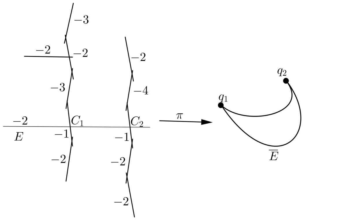
| Multiplicity seq. | ||
|---|---|---|
| HN pairs | ||
| Puiseux seq. | ||
| Puiseux pairs | ||
| Zariski pairs | ||
| Semigroups |
The Lemma 5.1 implies that is of HN-type . Other invariants and the graphs of the resolution can be computed easily using the results above. Their values are given in the table in Fig. 23.
Looking more carefully at the resolution of we see that the first three blowups (the second one is outer and the third one is inner with respect to the reduced preimage of ) are described by the HN pair . The next blowup is outer. After that the proper transform of is smooth, but we need another outer and inner blowup to make the total transform snc. These three blowups are described by the second HN-pair . Note that after the first three blowups, the cusp meets the last exceptional curve with multiplicity . Therefore (see the discussion preceding (2.4)), if we used HN-pairs as in [KPR16] instead of the standard ones, namely, if we required that and thus chose some general smooth germ transversal to the last exceptional curve instead of the maximally tangent one, then the HN-type would be . The fact that we have two Puiseux pairs (equivalently, that the Puiseux sequence is of length ) corresponds to the fact that the exceptional divisor over has one branching component.
Example 5.4 (Computation of other characteristics from HN-pairs).
Let , . Consider a rational cuspidal curve of HN-type . Its standard HN-pairs are
Lemma 5.1 gives Puiseux sequences
Puiseux pairs
and Zariski pairs
Topologically the cusps of are the same as the ones with Puiseux parametrization
To compute multiplicity sequences we either apply Lemma 2.11 or we simply follow the Euclidean algorithm using the fact when passing from a cusp to its proper transform under a blowup the initial HN-pair is replaced by . Let us make the computation. The multiplicity of equals . The first blowup replaces the first HN-pair with . The next blowups are centered at a point of multiplicity on the proper transforms of . After they are performed, the first HN-pair becomes , which means that the cusp of the proper transform of the germ of the curve is not at the intersection point of proper transforms of local coordinates used to define this HN-pair, so we move on to the next HN-pair . The latter describes blowups at a point of multiplicity on the proper transform of . Therefore, the multiplicity sequence of is
For the first blowups are centered at a point of multiplicity on the proper transforms of , and they replace the HN-pair by . As we have seen before, this HN-pair describes blowups at smooth points of the proper transforms of . Thus the multiplicity sequence of is
| degree | HN pairs (standard, except () for , or () for , see Rem. 1.4) | Multiplicity sequences | Parameters | References | |||
| [FZ96] | |||||||
| [CNKR09, (ii.1)], [BZ10, (e)] | |||||||
| [Ton12a, (3)] | |||||||
| [CNKR09, (ii.2)], [BZ10, (f)] | |||||||
| [Fen99, (4)], [Ton12a, (4)] | |||||||
| [CNKR09, (ii.4)], [BZ10, (c)] | |||||||
| [Fen99, (5)], [Ton12a, (2)] | |||||||
| [CNKR09, (ii.4)], [BZ10, (d)] | |||||||
| [Fen99, (6)], [Ton12a, (1)] | |||||||
| [BZ10, (s)], | |||||||
| [KP16, (a)] | |||||||
| [BZ10, (s)], | |||||||
| [KP16, (b)] | |||||||
| [tD95, VII], [Bod16, (b)] | |||||||
| [Ore02] | |||||||
| [Ore02] | |||||||
| where are the Fibonacci numbers defined by , , . | |||||||
References
- [BHPVdV04] Wolf P. Barth, Klaus Hulek, Chris A. M. Peters, and Antonius Van de Ven, Compact complex surfaces, second ed., Results in Mathematics and Related Areas. 3rd Series. A Series of Modern Surveys in Mathematics, vol. 4, Springer-Verlag, Berlin, 2004.
- [BL14] Maciej Borodzik and Charles Livingstone, Heegaard Floer homology and rational cuspidal curves, Forum Math. Sigma 2 (2014), e1, 28, arXiv:1304.1062.
- [Bod16] József Bodnár, Construction of bicuspidal rational complex projective plane curves, arXiv:1608.02921, 2016.
- [Bre93] Glen E. Bredon, Topology and geometry, Graduate Texts in Mathematics, Springer New York, 1993.
- [BZ10] Maciej Borodzik and Henryk Żoła̧dek, Complex algebraic plane curves via Poincaré-Hopf formula. II. Annuli, Israel J. Math. 175 (2010), 301–347, arXiv:0708.1661.
- [CNKR09] Pierrette Cassou-Nogues, Mariusz Koras, and Peter Russell, Closed embeddings of in . I, J. Algebra 322 (2009), no. 9, 2950–3002.
- [EN85] David Eisenbud and Walter Neumann, Three-dimensional link theory and invariants of plane curve singularities, Annals of Mathematics Studies, vol. 110, Princeton University Press, Princeton, NJ, 1985.
- [FdBLMHN07a] J. Fernández de Bobadilla, I. Luengo, A. Melle-Hernández, and A. Némethi, On rational cuspidal plane curves, open surfaces and local singularities, Singularity theory, World Sci. Publ., Hackensack, NJ, 2007, pp. 411–442.
- [FdBLMHN07b] Javier Fernández de Bobadilla, Ignacio Luengo, Alejandro Melle Hernández, and Andras Némethi, Classification of rational unicuspidal projective curves whose singularities have one Puiseux pair, Real and complex singularities, Trends Math., Birkhäuser, Basel, 2007, pp. 31–45.
- [Fen99] Torsten Fenske, Rational 1- and 2-cuspidal plane curves., Beiträge zur Algebra und Geometrie 40 (1999), no. 2, 309–329.
- [Fuj82] Takao Fujita, On the topology of noncomplete algebraic surfaces, J. Fac. Sci. Univ. Tokyo Sect. IA Math. 29 (1982), no. 3, 503–566.
- [FZ94] Hubert Flenner and Mikhail Zaidenberg, -acyclic surfaces and their deformations, Classification of algebraic varieties (L’Aquila, 1992), Contemp. Math., vol. 162, Amer. Math. Soc., Providence, RI, 1994, pp. 143–208.
- [FZ96] by same author, On a class of rational cuspidal plane curves, Manuscripta Math. 89 (1996), no. 4, 439–459.
- [FZ03] by same author, Rational curves and rational singularities, Math. Z. 244 (2003), no. 3, 549–575.
- [GLS07] G.-M. Greuel, C. Lossen, and E. Shustin, Introduction to singularities and deformations, Springer Monographs in Mathematics, Springer, Berlin, 2007.
- [GP99] R. V. Gurjar and C. R. Pradeep, -homology planes are rational. III, Osaka J. Math. 36 (1999), no. 2, 259–335.
- [Har77] Robin Hartshorne, Algebraic geometry, Springer-Verlag, New York, 1977, Graduate Texts in Mathematics, No. 52.
- [Iit82] Shigeru Iitaka, Algebraic geometry, Graduate Texts in Mathematics, vol. 76, Springer-Verlag, New York, 1982, An introduction to birational geometry of algebraic varieties, North-Holland Mathematical Library, 24.
- [Kas87] Hiroko Kashiwara, Fonctions rationnelles de type sur le plan projectif complexe, Osaka J. Math. 24 (1987), no. 3, 521–577.
- [KP15] Mariusz Koras and Karol Palka, The Coolidge–Nagata conjecture, arXiv:1502.07149, 2015.
- [KP16] by same author, Classification of sporadic -embeddings into , preprint, 2016.
- [KPR16] Mariusz Koras, Karol Palka, and Peter Russell, The geometry of sporadic -embeddings into , J. Algebra 456 (2016), 207–249, arXiv:1405.6872.
- [KR99] Mariusz Koras and Peter Russell, -actions on : the smooth locus of the quotient is not of hyperbolic type, J. Algebraic Geom. 8 (1999), no. 4, 603–694.
- [Liu14] Tiankai Liu, On planar rational cuspidal curves, Ph. D. thesis, http://hdl.handle.net/1721.1/90190, 2014.
- [Miy01] Masayoshi Miyanishi, Open algebraic surfaces, CRM Monograph Series, vol. 12, American Mathematical Society, Providence, RI, 2001.
- [Moe08] Karoline Torgunn Moe, Rational cuspidal curves, M.Sc. thesis, http://folk.uio.no/torgunnk/MOE_MASTER.pdf, 2008.
- [MS81] Masayoshi Miyanishi and Tohru Sugie, On a projective plane curve whose complement has logarithmic kodaira dimension , Osaka J. Math. 18 (1981), no. 1, 1–11.
- [MS91] by same author, -homology planes with -fibrations, Osaka J. Math. 28 (1991), no. 1, 1–26.
- [MT92] M. Miyanishi and S. Tsunoda, Absence of the affine lines on the homology planes of general type, J. Math. Kyoto Univ. 32 (1992), no. 3, 443–450.
- [Ore02] Stephan Yu. Orevkov, On rational cuspidal curves, Math. Ann. 324 (2002), no. 4, 657–673.
- [Pal12] Karol Palka, Classification of singular -homology planes II: - and -rulings, Pacific J. Math. 258 (2012), no. 2, 421–457, arXiv:1201.2463.
- [Pal14] by same author, The Coolidge–Nagata conjecture, part I, Adv. Math. 267 (2014), 1–43, arXiv:1405.5917.
- [Pal15] by same author, A new proof of the theorems of Lin-Zaidenberg and Abhyankar-Moh-Suzuki, J. Algebra Appl. 14 (2015), No. 8, arXiv:1405.5391.
- [Pal16] by same author, Cuspidal curves, minimal models and Zaidenberg’s finiteness conjecture, Journal für die reine und angewandte Mathematik (Crelles Journal) (2016), arXiv:1405.5346.
- [Rus80] Peter Russell, Hamburger-Noether expansions and approximate roots of polynomials, Manuscripta Math. 31 (1980), no. 1-3, 25–95.
- [Suz77] Masakazu Suzuki, Sur les opérations holomorphes du groupe additif complexe sur l’espace de deux variables complexes, Ann. Sci. École Norm. Sup. (4) 10 (1977), no. 4, 517–546.
- [tD95] Tammo tom Dieck, Letter to H. Flenner, 1995.
- [Ton00] Keita Tono, Defining equations of certain rational cuspidal plane curves, Doctoral thesis, Saitama University, 2000.
- [Ton01] by same author, Rational unicuspidal plane curves with , Newton polyhedrons and Singularities, vol. 1233, RIMS Kokyuroku, 2001, pp. 82–89.
- [Ton12a] by same author, On a new class of rational cuspidal plane curves with two cusps, arXiv:1205.1248, 2012.
- [Ton12b] by same author, On Orevkov’s rational cuspidal plane curves, J. Math. Soc. Japan 64 (2012), no. 2, 365–385.
- [Ton12c] by same author, On the self-intersection number of the nonsingular models of rational cuspidal plane curves, arXiv:1408.0190, 2012.
- [Tsu81] Shuichiro Tsunoda, The complements of projective plane curves, vol. 446, RIMS Kokyuroku, 1981, pp. 48–56.
- [Wal04] Charles Terence Clegg Wall, Singular points of plane curves, London Mathematical Society Student Texts, Cambridge University Press, 2004.
- [Zai87] Mikhail Zaidenberg, Isotrivial families of curves on affine surfaces, and the characterization of the affine plane, Izv. Akad. Nauk SSSR Ser. Mat. 51 (1987), no. 3, 534–567, 688.